Most tabular models are trained in Python and used somewhere else. The features live in a warehouse, the scores are needed in that same warehouse (for a dashboard, a campaign list, a risk report, or a downstream join), and the usual answer is a pipeline that exports rows, scores them in a Python service, and writes the scores back. That round trip is slow to build, fragile to operate, and a governance headache, because customer data leaves the system whose access controls and audit logs were designed to protect it.
In-database scoring inverts the flow. Instead of moving the data to the model, it moves the model to the data, by expressing the fitted model as something the database can execute natively: a SQL expression, a user-defined function, or a call into a model runtime embedded in the engine. This chapter explains why and when to do it, how a fitted scikit-learn pipeline becomes SQL, how the main deployment options compare, and, most importantly, how to prove that the database computes the same scores as Python. The runnable part builds a pipeline-to-SQL translator by hand, executes the result in SQLite, and tests parity, so that the automatic tools introduced afterward are no longer black boxes.
282.1 Why Score Where the Data Lives
Data gravity. Large tables are expensive to move. Scoring millions of rows in place avoids extraction jobs, network transfer, egress charges, and a second copy of sensitive data in a serving system.
Governance. Inside the warehouse, scoring inherits existing role-based access control, row and column security, lineage, and audit logging. A score computed by a view is versioned with the view definition and can be reproduced for a regulator by rerunning the query against a historical snapshot.
Consistency. When features are defined in SQL and scores are computed in the same query, the model sees exactly the feature values the business sees. A separate Python serving path is a classic source of training-serving skew, where subtly different feature code in two places produces different inputs (Sculley et al. 2015).
Operational simplicity. A scoring view needs no container, no autoscaling, and no on-call rotation beyond the warehouse itself. Batch scoring becomes a scheduled INSERT ... SELECT.
In-database scoring is not free. SQL is a poor language for models with dynamic control flow, large embeddings, or GPU-bound computation, and a warehouse is the wrong place for low-latency online inference behind an API. The database research literature has argued for decades that analytics should run inside the engine, from user-defined aggregates for statistical models (Ordonez 2010) to full in-database machine learning libraries (Hellerstein et al. 2012), and recent systems go further by optimizing data and model operators together in one query plan (Karanasos et al. 2020, Park et al. 2022).
282.2 The Options
There are four broad ways to run a trained model inside a database.
Compile the model to plain SQL. Linear models become arithmetic expressions, one-hot encoders and trees become CASE WHEN expressions, and ensembles become sums of trees. The result runs on any engine with no extra runtime, uses the engine’s optimizer and parallelism, and is fully transparent. The Posit orbital library automates this for scikit-learn pipelines, using ONNX as an intermediate representation and emitting SQL for many dialects through the sqlglot library.
Run Python inside the database as a user-defined function (UDF). Snowflake (Snowpark Python UDFs and vectorized UDFs), BigQuery (remote functions), Databricks, and PostgreSQL (PL/Python) can execute Python next to the data. This supports any model, at the price of a Python sandbox, package management, and per-batch serialization overhead.
Call a native model runtime. Several engines can load a serialized model, often in ONNX format, and evaluate it with an embedded runtime. BigQuery ML can import ONNX and other external models for ML.PREDICT, and research prototypes such as Raven integrate ONNX Runtime directly into the query processor of SQL Server (Karanasos et al. 2020). Compilers such as Hummingbird translate traditional models into tensor programs that such runtimes, and GPUs, execute efficiently (Nakandala et al. 2020).
Train in the database. BigQuery ML, Snowflake ML functions, and MADlib on PostgreSQL train and score with SQL syntax. This avoids translation entirely but restricts you to the algorithms and preprocessing the platform provides.
For the models that dominate tabular production work (regularized linear and logistic regression, single trees, and tree ensembles of moderate size), option 1 is often the best default, and it is the one this chapter builds from first principles.
282.3 From Pipeline to SQL: The Math
Consider a typical scikit-learn pipeline for a binary outcome: numeric features are median-imputed and standardized, categorical features are one-hot encoded with unknown categories ignored, and a logistic regression produces a probability. For numeric feature \(j\) with training median \(\tilde{x}_j\), mean \(\mu_j\), and scale \(\sigma_j\), and categorical feature \(k\) with levels \(\mathcal{C}_k\), the linear predictor is \[
\eta(\mathbf{x}) = b + \sum_{j} w_j \,\frac{\operatorname{impute}(x_j) - \mu_j}{\sigma_j} + \sum_{k}\sum_{c \in \mathcal{C}_k} v_{k,c}\, \mathbb{1}[x_k = c],
\qquad
p(\mathbf{x}) = \frac{1}{1 + e^{-\eta(\mathbf{x})}} .
\] Each piece has a direct SQL counterpart. Imputation is COALESCE(x, median). Standardization is arithmetic. The indicator sum for one categorical feature is a single CASE x WHEN 'a' THEN v_a WHEN 'b' THEN v_b ELSE 0 END, where the ELSE 0 branch reproduces handle_unknown="ignore", since an unseen category activates no column. The constants can be folded, which shortens the SQL: \[
\eta(\mathbf{x}) = \underbrace{b - \sum_j \frac{w_j \mu_j}{\sigma_j}}_{b'} + \sum_j \frac{w_j}{\sigma_j}\operatorname{impute}(x_j) + \sum_k \sum_c v_{k,c}\,\mathbb{1}[x_k = c] .
\] A decision tree is a nested conditional. Each internal node tests \(x_f \le t\) and each leaf returns a class probability, so the tree becomes nested CASE WHEN x_f <= t THEN ... ELSE ... END. A gradient-boosted ensemble with \(M\) trees and learning rate folded into the leaves is \(\eta(\mathbf{x}) = b + \sum_{m=1}^{M} \text{tree}_m(\mathbf{x})\), a sum of \(M\) such expressions. The SQL grows with the total number of leaves, which is why tools offer options such as emitting each tree as a separate subexpression.
How much numerical error is acceptable? SQL and NumPy both use IEEE double precision, but they add terms in different orders, and a translator must print every constant as decimal text. Floating-point addition is not associative, so differences at the level of machine epsilon are expected and harmless (Goldberg 1991). Printing constants with too few digits is not harmless. If the literal for \(w_j\) is off by \(\delta_j\), the linear predictor moves by \(\sum_j \delta_j x_j\), and since \(\mathrm{d}p/\mathrm{d}\eta = p(1-p) \le \tfrac14\), \[
|\Delta p| \le \tfrac14\, |\Delta \eta| \le \tfrac14 \sum_j |\delta_j|\,|x_j| .
\] Printing every float with Python’s repr produces the shortest decimal string that round-trips to the identical double, which removes this error source entirely.
282.4 Building the Translator
We start with a synthetic customer churn table with numeric and categorical features and some missing values, and fit the pipeline described above.
train rows 4500, test rows 1500, churn rate 0.271
test accuracy 0.792
The translator reads the fitted parameters out of each step and writes the folded expression. It handles exactly the steps in this pipeline and refuses anything else, which is the right behavior for a hand-written translator: silently mistranslating an unsupported step is far worse than failing loudly.
Code
def lit(x: float, digits: int|None=None) ->str:"""SQL literal for a float. repr() round-trips exactly. `digits` rounds on purpose."""returnrepr(float(x)) if digits isNoneelsef"{float(x):.{digits}g}"def quote(s: str) ->str:return"'"+str(s).replace("'", "''") +"'"def logistic_pipeline_to_sql(pipe, table, id_col, digits=None, impute=True): prep, clf = pipe.named_steps["prep"], pipe.named_steps["clf"] coef, intercept = clf.coef_.ravel(), float(clf.intercept_[0]) terms, pos = [], 0for name, trans, cols in prep.transformers_:if name =="remainder":continueif name =="num": imp, sc = trans.named_steps["impute"], trans.named_steps["scale"]assertisinstance(imp, SimpleImputer) andisinstance(sc, StandardScaler)for j, col inenumerate(cols): w = coef[pos + j] / sc.scale_[j] intercept -= w * sc.mean_[j] x =f"COALESCE({col}, {lit(imp.statistics_[j], digits)})"if impute else col terms.append(f"{lit(w, digits)} * {x}") pos +=len(cols)elif name =="cat":assertisinstance(trans, OneHotEncoder) and trans.handle_unknown =="ignore"for col, cats inzip(cols, trans.categories_): whens =" ".join(f"WHEN {quote(c)} THEN {lit(coef[pos + i], digits)}"for i, c inenumerate(cats)) terms.append(f"(CASE {col}{whens} ELSE 0.0 END)") pos +=len(cats)else:raiseNotImplementedError(f"cannot translate transformer {name!r}")assert pos ==len(coef), "every coefficient must be consumed exactly once" logit =f"{lit(intercept, digits)}\n + "+"\n + ".join(terms)return (f"SELECT {id_col},\n logit,\n 1.0 / (1.0 + exp(-logit)) AS p_churn\n"f"FROM (SELECT {id_col},\n{logit} AS logit\n FROM {table})")sql = logistic_pipeline_to_sql(pipe, "customers", "customer_id")print(sql)
SELECT customer_id,
       logit,
       1.0 / (1.0 + exp(-logit)) AS p_churn
FROM (SELECT customer_id,
    -0.6409024237874327
    + -0.046889996743514344 * COALESCE(tenure, 36.0)
    + 0.020721141987379246 * COALESCE(monthly_charges, 69.415)
    + -1.2036619183631716e-05 * COALESCE(total_charges, 2030.21)
    + (CASE contract WHEN 'month-to-month' THEN 0.6815168418194233 WHEN 'one-year' THEN -0.27947618891885323 WHEN 'two-year' THEN -1.281194300317162 ELSE 0.0 END)
    + (CASE payment_method WHEN 'bank transfer' THEN -0.45102522683005963 WHEN 'card' THEN -0.30956584637222245 WHEN 'cash' THEN -0.30103018583665453 WHEN 'e-wallet' THEN 0.18246761162234884 ELSE 0.0 END)
    + (CASE internet_service WHEN 'dsl' THEN -0.41991012775643183 WHEN 'fiber' THEN -0.06503352857559878 WHEN 'none' THEN -0.3942099910845594 ELSE 0.0 END) AS logit
  FROM customers)
The output is a single readable query. Every number in it is a fitted parameter, and every line corresponds to one feature, so a reviewer who knows SQL but not scikit-learn can audit what the model does.
282.5 Testing Parity
A translated model is only trustworthy if it is tested against the original on the same rows. We load the test set into an in-memory SQLite database, run the query, and compare against predict_proba and decision_function row by row. SQLite stands in for the warehouse here. The test logic is identical against Snowflake, BigQuery, or PostgreSQL.
Code
con = sqlite3.connect(":memory:")try: con.execute("SELECT exp(1.0)").fetchone()except sqlite3.OperationalError: # SQLite built without math functionsimport math con.create_function("exp", 1, math.exp, deterministic=True)test[["customer_id"] + num_cols + cat_cols].to_sql("customers", con, index=False)def score_sql(query): out = pd.read_sql_query(query, con).set_index("customer_id")return out.loc[test["customer_id"]]def parity_report(sql_scores, label): X = test[num_cols + cat_cols] p_py = pipe.predict_proba(X)[:, 1] eta_py = pipe.decision_function(X) p_sql = sql_scores["p_churn"].to_numpy(dtype=float) ok =~np.isnan(p_sql) # compare only rows that received a scorereturn {"translation": label,"null scores": int((~ok).sum()),"max |logit diff|": np.abs(sql_scores["logit"].to_numpy(dtype=float)[ok] - eta_py[ok]).max(),"max |p diff|": np.abs(p_sql[ok] - p_py[ok]).max(),"label flips at 0.5": int(((p_sql[ok] >=0.5) != (p_py[ok] >=0.5)).sum())}t0 = time.perf_counter()exact = score_sql(sql)elapsed = time.perf_counter() - t0reports = [parity_report(exact, "exact literals")]naive = score_sql(logistic_pipeline_to_sql(pipe, "customers", "customer_id", impute=False))reports.append(parity_report(naive, "no COALESCE"))print(pd.DataFrame(reports).set_index("translation"))print(f"\nscored {len(exact)} rows in SQLite in {elapsed *1000:.1f} ms")
                null scores  max |logit diff|  max |p diff|  label flips at 0.5
translation
exact literals            0      8.881784e-16  2.220446e-16                   0
no COALESCE              54      8.881784e-16  2.220446e-16                   0

scored 1500 rows in SQLite in 4.9 ms
The exact translation agrees with Python to within floating-point rounding on every row. The naive translation, which omits the COALESCE that implements the imputer, returns NULL for every row with a missing value, because SQL arithmetic propagates NULL. This is the most common real-world translation bug, and it is silent: the query succeeds, the scores for complete rows are perfect, and the missing scores show up weeks later as customers who were never contacted.
Edge cases deserve their own tests, because the test split may not contain them. Below we score rows with an unseen payment method, a missing value, and extreme numeric values.
Unseen categories contribute zero in both systems, missing values are imputed identically, and extreme inputs saturate the sigmoid in both. Saturation is benign for SQLite’s exp, but some engines raise an overflow error for exp of a large positive number, so production SQL often clips the logit to a range such as \([-30, 30]\) before exponentiating.
282.5.1 Literal precision
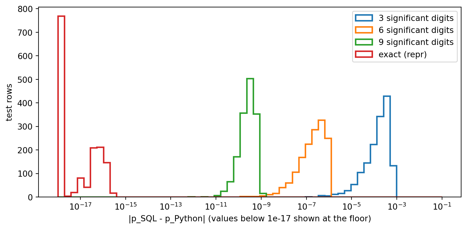
The next experiment isolates the error from printing constants with too few significant digits, which is what a hand-written translation or a careless code generator does.
Code
p_py = pipe.predict_proba(test[num_cols + cat_cols])[:, 1]diffs, rows = {}, []for digits in [3, 6, 9, None]: label ="exact (repr)"if digits isNoneelsef"{digits} significant digits" s = score_sql(logistic_pipeline_to_sql(pipe, "customers", "customer_id", digits=digits)) d = np.abs(s["p_churn"].to_numpy(dtype=float) - p_py) diffs[label] = np.maximum(d, 1e-18) # floor so exact zeros plot on log axis rows.append({"literals": label, "max |p diff|": d.max(), "median |p diff|": np.median(d),"label flips at 0.5": int(((s["p_churn"].to_numpy() >=0.5) != (p_py >=0.5)).sum())})print(pd.DataFrame(rows).set_index("literals"))fig, ax = plt.subplots(figsize=(8, 4))bins = np.logspace(-18, -1, 60)for label, d in diffs.items(): ax.hist(d, bins=bins, histtype="step", linewidth=1.8, label=label)ax.set_xscale("log")ax.set_xlabel("|p_SQL - p_Python| (values below 1e-17 shown at the floor)")ax.set_ylabel("test rows")ax.legend()fig.tight_layout()plt.show()
Figure 282.1: Absolute difference between Python and SQL churn probabilities on the test set when model constants are printed with 3, 6, or 9 significant digits, or with exact round-trip literals. Rounded literals introduce errors many orders of magnitude above floating-point rounding.
Each added digit shrinks the error by roughly the expected factor, yet every rounded variant stays far above the rounding floor. Whether a given error flips a decision depends on how many customers sit that close to a threshold. On a test set of this size it may be none, but across millions of scored customers some always will, and rankings used for targeting shift as well. Exact literals leave only the unavoidable rounding from a different summation order. The lesson is to generate SQL programmatically with exact literals and to set the parity tolerance close to machine precision, so that any real translation error stands out.
282.5.2 Trees and a subtle float32 trap
A decision tree translates into nested CASE expressions. The same parity test applies, with one twist worth knowing about: scikit-learn’s tree estimators convert their input to 32-bit floats before comparing it with the (64-bit) thresholds, while SQL compares in 64-bit arithmetic. Values extremely close to a threshold can therefore be routed differently.
Code
tree_pipe = Pipeline([ ("prep", ColumnTransformer([ ("num", SimpleImputer(strategy="median"), num_cols), ("cat", OneHotEncoder(handle_unknown="ignore"), cat_cols), ])), ("tree", DecisionTreeClassifier(max_depth=4, min_samples_leaf=50, random_state=0)),]).fit(train[num_cols + cat_cols], train["churn"])prep_t = tree_pipe.named_steps["prep"]feature_sql = [f"COALESCE({c}, {lit(m)})"for c, m inzip(num_cols, prep_t.named_transformers_["num"].statistics_)]for col, cats inzip(cat_cols, prep_t.named_transformers_["cat"].categories_): feature_sql += [f"(CASE WHEN {col} = {quote(c)} THEN 1.0 ELSE 0.0 END)"for c in cats]t = tree_pipe.named_steps["tree"].tree_def node_sql(i, indent=2): pad =" "* indentif t.children_left[i] ==-1: # leaf: class-1 probability v = t.value[i, 0]return lit(v[1] / v.sum())return (f"CASE WHEN {feature_sql[t.feature[i]]} <= {lit(t.threshold[i])}\n"f"{pad}THEN {node_sql(t.children_left[i], indent +2)}\n"f"{pad}ELSE {node_sql(t.children_right[i], indent +2)} END")tree_sql =f"SELECT customer_id, {node_sql(0)} AS p_churn FROM customers"s_tree = pd.read_sql_query(tree_sql, con).set_index("customer_id").loc[test["customer_id"]]p_tree = tree_pipe.predict_proba(test[num_cols + cat_cols])[:, 1]print(f"tree leaves: {t.n_leaves}, SQL length: {len(tree_sql)} characters")print(f"max |p diff| on the test set: {np.abs(s_tree['p_churn'].to_numpy() - p_tree).max():.2e}")# Probe every numeric threshold with the smallest double just above it.probes =0for i in np.where(t.children_left !=-1)[0]: f = t.feature[i]if f >=len(num_cols):continue# one-hot splits are 0/1 only x_above = np.nextafter(t.threshold[i], np.inf) sklearn_goes_left = np.float32(x_above) <= t.threshold[i] probes +=int(sklearn_goes_left) # SQL always goes right heren_numeric =int(sum(t.feature[i] <len(num_cols) for i in np.where(t.children_left !=-1)[0]))print(f"numeric thresholds where a value just above the threshold is routed "f"differently by scikit-learn and SQL: {probes} of {n_numeric}")
tree leaves: 16, SQL length: 1704 characters
max |p diff| on the test set: 0.00e+00
numeric thresholds where a value just above the threshold is routed differently by scikit-learn and SQL: 7 of 11
On real data the tree scores agree exactly, because observed values almost never land within a 32-bit rounding step of a threshold. The probe shows that for a fraction of thresholds a disagreeing input exists: a value a hair above the threshold, which SQL sends right and scikit-learn, after rounding to 32 bits, sends left. ONNX-based tools typically compute in 32-bit floats as well, so the same caution applies to them, and practitioners have reported rare prediction differences of exactly this kind. The defensible approach is a parity test with a small tolerance on probabilities plus a monitored count of label disagreements, not an assumption of bitwise equality.
282.6 Automating the Translation
Writing translators by hand is instructive but does not scale to many model types. The orbital library converts a fitted scikit-learn pipeline into SQL automatically. It parses the pipeline (internally via ONNX) given the column types, and exports SQL for a chosen dialect. The chunk below shows the workflow against Snowflake with Snowpark. It requires the packages and a Snowflake account, so it is not executed here.
Code
# Requires: pip install orbital snowflake-snowpark-python, and a Snowflake account.import osimport orbitalimport orbital.typesfrom snowflake.snowpark import Sessionfeatures = {c: orbital.types.DoubleColumnType() for c in num_cols}features.update({c: orbital.types.StringColumnType() for c in cat_cols})parsed = orbital.parse_pipeline(pipe, features=features)churn_sql = orbital.export_sql("CUSTOMERS", parsed, dialect="snowflake")print(churn_sql[:1000])# Credentials come from the environment or a secrets manager, never from the notebook.session = Session.builder.configs({"account": os.environ["SNOWFLAKE_ACCOUNT"],"user": os.environ["SNOWFLAKE_USER"],"authenticator": "externalbrowser","role": "ML_ROLE", "warehouse": "SCORING_WH", "database": "ML_DB", "schema": "PUBLIC",}).create()# A view makes the model a governed, versioned database object.session.sql(f"CREATE OR REPLACE VIEW CUSTOMER_CHURN_SCORES AS {churn_sql}").collect()# Parity test in CI: score a fixed sample in both systems and compare.sample = session.table("CUSTOMERS_PARITY_SAMPLE").to_pandas()sql_scores = session.sql(orbital.export_sql("CUSTOMERS_PARITY_SAMPLE", parsed, dialect="snowflake")).to_pandas()
The same parsed pipeline exports to other dialects by changing the dialect argument, which is what makes this approach portable across warehouses. orbital describes itself as a work in progress and lists the models it supports. Not every transformer and model can be represented as SQL, so pin the library version, check the supported list for that version, and keep the parity test running in CI.
When a model cannot be expressed as SQL, the alternatives are to export it to ONNX and run it with an embedded runtime, or to register it as a Python model that the warehouse runs in a sandbox. Both are shown below for completeness, again without execution.
Code
# ONNX export and scoring with onnxruntime. Requires: pip install skl2onnx onnxruntimeimport onnxruntime as ortfrom skl2onnx import convert_sklearnfrom skl2onnx.common.data_types import FloatTensorType, StringTensorTypeinitial_types = ([(c, FloatTensorType([None, 1])) for c in num_cols]+ [(c, StringTensorType([None, 1])) for c in cat_cols])onx = convert_sklearn(pipe, initial_types=initial_types)sess = ort.InferenceSession(onx.SerializeToString())inputs = {c: test[[c]].to_numpy(dtype=np.float32) for c in num_cols}inputs.update({c: test[[c]].to_numpy(dtype=object) for c in cat_cols})p_onnx = sess.run(None, inputs)[1] # probabilities (float32 arithmetic)# Snowflake Model Registry: Snowflake runs the Python model next to the data.from snowflake.ml.registry import Registryregistry = Registry(session=session)mv = registry.log_model(pipe, model_name="CHURN_LOGREG", version_name="V1", sample_input_data=train[num_cols + cat_cols].head(100))scores = mv.run(session.table("CUSTOMERS"), function_name="predict_proba")
282.7 Pitfalls and When to Use
Test parity, always, and on purpose-built edge cases. Compare Python and SQL scores row by row on a fixed sample that includes missing values, unseen categories, boundary values, and extreme values. Fail the build on any NULL score, on probability differences above a tolerance near machine precision for SQL-compiled linear models, or on any change in predicted label beyond a small allowance for tree models evaluated in 32-bit arithmetic.
Missing values are the most common bug. SQL NULL propagates through arithmetic and fails every comparison, so x <= t is neither true nor false for a missing x. Make every imputation explicit with COALESCE, and decide deliberately which branch a missing value takes in a tree.
Categories must match exactly. String comparison in SQL is sensitive to case, whitespace, and collation settings, which may differ from Python. Normalize categorical values with the same function on both sides, and test that a category that looks the same in a dashboard actually matches.
Print constants exactly. Use round-trip float formatting. Rounded literals are a silent source of error that grows with feature magnitude.
Mind numerical limits of the engine. Clip logits before exp, watch integer division in engines where 1/2 is zero, and check decimal types, since some warehouses default numeric literals to fixed-point decimals with limited scale.
Version the SQL with the model. The generated view is the deployed model. Store it in version control next to the training code and the parity test, and record the model version as a column in the scored output, so that every score can be traced to the exact model that produced it.
Know when not to do it. Deep networks, large embeddings, text models, and low-latency online scoring belong in a model server or a dedicated runtime. In-database scoring shines for batch and near-real-time scoring of tabular models over data that already lives in the warehouse, which describes a large share of production machine learning in practice.
282.8 References
Sculley, D., Holt, G., Golovin, D., Davydov, E., Phillips, T., Ebner, D., Chaudhary, V., Young, M., Crespo, J.-F., and Dennison, D. “Hidden Technical Debt in Machine Learning Systems.” Advances in Neural Information Processing Systems 28, 2015, 2503-2511. https://proceedings.neurips.cc/paper/2015/hash/86df7dcfd896fcaf2674f757a2463eba-Abstract.html
Ordonez, C. “Statistical Model Computation with UDFs.” IEEE Transactions on Knowledge and Data Engineering 22(12), 2010, 1752-1765. https://doi.org/10.1109/TKDE.2010.44
Hellerstein, J. M., Ré, C., Schoppmann, F., Wang, D. Z., Fratkin, E., Gorajek, A., Ng, K. S., Welton, C., Feng, X., Li, K., and Kumar, A. “The MADlib Analytics Library or MAD Skills, the SQL.” Proceedings of the VLDB Endowment 5(12), 2012, 1700-1711. https://doi.org/10.14778/2367502.2367519
Karanasos, K., Interlandi, M., Psallidas, F., Sen, R., Park, K., Popivanov, I., Xin, D., Nakandala, S., et al. “Extending Relational Query Processing with ML Inference.” Conference on Innovative Data Systems Research (CIDR), 2020. https://vldb.org/cidrdb/2020/extending-relational-query-processing-with-ml-inference.html
Park, K., Saur, K., Banda, D., Sen, R., Interlandi, M., and Karanasos, K. “End-to-end Optimization of Machine Learning Prediction Queries.” Proceedings of the 2022 International Conference on Management of Data (SIGMOD), 2022. https://doi.org/10.1145/3514221.3526141
Nakandala, S., Saur, K., Yu, G.-I., Karanasos, K., Curino, C., Weimer, M., and Interlandi, M. “A Tensor Compiler for Unified Machine Learning Prediction Serving.” 14th USENIX Symposium on Operating Systems Design and Implementation (OSDI), 2020, 899-917. https://www.usenix.org/conference/osdi20/presentation/nakandala
Goldberg, D. “What Every Computer Scientist Should Know About Floating-Point Arithmetic.” ACM Computing Surveys 23(1), 1991, 5-48. https://doi.org/10.1145/103162.103163
Pedregosa, F. et al. “Scikit-learn: Machine Learning in Python.” Journal of Machine Learning Research 12, 2011, 2825-2830. https://jmlr.org/papers/v12/pedregosa11a.html
How to cite this chapter
Nguyen, M. (2026). Scoring Models Inside the Database. In AI in Action: A Reference for Artificial Intelligence. https://mikenguyen13.github.io/ai_in_action/1210-in-database-model-scoring.html
BibTeX
@incollection{nguyen2026aiinaction-1210indatabasemodelscoring,
  author    = {Nguyen, Mike},
  title     = {{Scoring Models Inside the Database}},
  booktitle = {{AI in Action: A Reference for Artificial Intelligence}},
  year      = {2026},
  url       = {https://mikenguyen13.github.io/ai_in_action/1210-in-database-model-scoring.html},
  note      = {Online book}
}
Source Code
# Scoring Models Inside the Database {#sec-in-database-scoring}Most tabular models are trained in Python and used somewhere else. The features live in a warehouse, the scores are needed in that same warehouse (for a dashboard, a campaign list, a risk report, or a downstream join), and the usual answer is a pipeline that exports rows, scores them in a Python service, and writes the scores back. That round trip is slow to build, fragile to operate, and a governance headache, because customer data leaves the system whose access controls and audit logs were designed to protect it.**In-database scoring** inverts the flow. Instead of moving the data to the model, it moves the model to the data, by expressing the fitted model as something the database can execute natively: a SQL expression, a user-defined function, or a call into a model runtime embedded in the engine. This chapter explains why and when to do it, how a fitted scikit-learn pipeline becomes SQL, how the main deployment options compare, and, most importantly, how to *prove* that the database computes the same scores as Python. The runnable part builds a pipeline-to-SQL translator by hand, executes the result in SQLite, and tests parity, so that the automatic tools introduced afterward are no longer black boxes.## Why Score Where the Data Lives**Data gravity.** Large tables are expensive to move. Scoring millions of rows in place avoids extraction jobs, network transfer, egress charges, and a second copy of sensitive data in a serving system.**Governance.** Inside the warehouse, scoring inherits existing role-based access control, row and column security, lineage, and audit logging. A score computed by a view is versioned with the view definition and can be reproduced for a regulator by rerunning the query against a historical snapshot.**Consistency.** When features are defined in SQL and scores are computed in the same query, the model sees exactly the feature values the business sees. A separate Python serving path is a classic source of **training-serving skew**, where subtly different feature code in two places produces different inputs (Sculley et al. 2015).**Operational simplicity.** A scoring view needs no container, no autoscaling, and no on-call rotation beyond the warehouse itself. Batch scoring becomes a scheduled `INSERT ... SELECT`.In-database scoring is not free. SQL is a poor language for models with dynamic control flow, large embeddings, or GPU-bound computation, and a warehouse is the wrong place for low-latency online inference behind an API. The database research literature has argued for decades that analytics should run inside the engine, from user-defined aggregates for statistical models (Ordonez 2010) to full in-database machine learning libraries (Hellerstein et al. 2012), and recent systems go further by optimizing data and model operators together in one query plan (Karanasos et al. 2020, Park et al. 2022).## The OptionsThere are four broad ways to run a trained model inside a database.1. **Compile the model to plain SQL.** Linear models become arithmetic expressions, one-hot encoders and trees become `CASE WHEN` expressions, and ensembles become sums of trees. The result runs on any engine with no extra runtime, uses the engine's optimizer and parallelism, and is fully transparent. The Posit `orbital` library automates this for scikit-learn pipelines, using ONNX as an intermediate representation and emitting SQL for many dialects through the sqlglot library.2. **Run Python inside the database as a user-defined function (UDF).** Snowflake (Snowpark Python UDFs and vectorized UDFs), BigQuery (remote functions), Databricks, and PostgreSQL (PL/Python) can execute Python next to the data. This supports any model, at the price of a Python sandbox, package management, and per-batch serialization overhead.3. **Call a native model runtime.** Several engines can load a serialized model, often in ONNX format, and evaluate it with an embedded runtime. BigQuery ML can import ONNX and other external models for `ML.PREDICT`, and research prototypes such as Raven integrate ONNX Runtime directly into the query processor of SQL Server (Karanasos et al. 2020). Compilers such as Hummingbird translate traditional models into tensor programs that such runtimes, and GPUs, execute efficiently (Nakandala et al. 2020).4. **Train in the database.** BigQuery ML, Snowflake ML functions, and MADlib on PostgreSQL train and score with SQL syntax. This avoids translation entirely but restricts you to the algorithms and preprocessing the platform provides.For the models that dominate tabular production work (regularized linear and logistic regression, single trees, and tree ensembles of moderate size), option 1 is often the best default, and it is the one this chapter builds from first principles.## From Pipeline to SQL: The MathConsider a typical scikit-learn pipeline for a binary outcome: numeric features are median-imputed and standardized, categorical features are one-hot encoded with unknown categories ignored, and a logistic regression produces a probability. For numeric feature $j$ with training median $\tilde{x}_j$, mean $\mu_j$, and scale $\sigma_j$, and categorical feature $k$ with levels $\mathcal{C}_k$, the linear predictor is$$\eta(\mathbf{x}) = b + \sum_{j} w_j \,\frac{\operatorname{impute}(x_j) - \mu_j}{\sigma_j} + \sum_{k}\sum_{c \in \mathcal{C}_k} v_{k,c}\, \mathbb{1}[x_k = c],\qquadp(\mathbf{x}) = \frac{1}{1 + e^{-\eta(\mathbf{x})}} .$$Each piece has a direct SQL counterpart. Imputation is `COALESCE(x, median)`. Standardization is arithmetic. The indicator sum for one categorical feature is a single `CASE x WHEN 'a' THEN v_a WHEN 'b' THEN v_b ELSE 0 END`, where the `ELSE 0` branch reproduces `handle_unknown="ignore"`, since an unseen category activates no column. The constants can be folded, which shortens the SQL:$$\eta(\mathbf{x}) = \underbrace{b - \sum_j \frac{w_j \mu_j}{\sigma_j}}_{b'} + \sum_j \frac{w_j}{\sigma_j}\operatorname{impute}(x_j) + \sum_k \sum_c v_{k,c}\,\mathbb{1}[x_k = c] .$$A decision tree is a nested conditional. Each internal node tests $x_f \le t$ and each leaf returns a class probability, so the tree becomes nested `CASE WHEN x_f <= t THEN ... ELSE ... END`. A gradient-boosted ensemble with $M$ trees and learning rate folded into the leaves is $\eta(\mathbf{x}) = b + \sum_{m=1}^{M} \text{tree}_m(\mathbf{x})$, a sum of $M$ such expressions. The SQL grows with the total number of leaves, which is why tools offer options such as emitting each tree as a separate subexpression.**How much numerical error is acceptable?** SQL and NumPy both use IEEE double precision, but they add terms in different orders, and a translator must print every constant as decimal text. Floating-point addition is not associative, so differences at the level of machine epsilon are expected and harmless (Goldberg 1991). Printing constants with too few digits is not harmless. If the literal for $w_j$ is off by $\delta_j$, the linear predictor moves by $\sum_j \delta_j x_j$, and since $\mathrm{d}p/\mathrm{d}\eta = p(1-p) \le \tfrac14$,$$|\Delta p| \le \tfrac14\, |\Delta \eta| \le \tfrac14 \sum_j |\delta_j|\,|x_j| .$$Printing every float with Python's `repr` produces the shortest decimal string that round-trips to the identical double, which removes this error source entirely.## Building the TranslatorWe start with a synthetic customer churn table with numeric and categorical features and some missing values, and fit the pipeline described above.```{python}#| label: code-1210-fitimport sqlite3import timeimport numpy as npimport pandas as pdimport matplotlib.pyplot as pltfrom sklearn.compose import ColumnTransformerfrom sklearn.impute import SimpleImputerfrom sklearn.linear_model import LogisticRegressionfrom sklearn.model_selection import train_test_splitfrom sklearn.pipeline import Pipelinefrom sklearn.preprocessing import OneHotEncoder, StandardScalerfrom sklearn.tree import DecisionTreeClassifierpd.set_option("display.width", 120)rng = np.random.default_rng(1210)n =6000contract = rng.choice(["month-to-month", "one-year", "two-year"], n, p=[0.55, 0.25, 0.20])payment = rng.choice(["card", "bank transfer", "e-wallet", "cash"], n)internet = rng.choice(["fiber", "dsl", "none"], n, p=[0.45, 0.40, 0.15])tenure = rng.integers(0, 73, n).astype(float)monthly = np.round(rng.uniform(18, 120, n), 2)total = np.round(tenure * monthly * rng.uniform(0.9, 1.1, n), 2)total[rng.random(n) <0.04] = np.nan # missing for some new accountseta = (-0.6-0.045* tenure +0.018* monthly+ np.select([contract =="one-year", contract =="two-year"], [-1.0, -2.0], 0.0)+ np.where(payment =="e-wallet", 0.5, 0.0) + np.where(internet =="fiber", 0.4, 0.0))churn = (rng.random(n) <1/ (1+ np.exp(-eta))).astype(int)df = pd.DataFrame({"customer_id": np.arange(n), "tenure": tenure, "monthly_charges": monthly,"total_charges": total, "contract": contract, "payment_method": payment,"internet_service": internet, "churn": churn})num_cols = ["tenure", "monthly_charges", "total_charges"]cat_cols = ["contract", "payment_method", "internet_service"]train, test = train_test_split(df, test_size=0.25, random_state=0, stratify=df["churn"])pipe = Pipeline([ ("prep", ColumnTransformer([ ("num", Pipeline([("impute", SimpleImputer(strategy="median")), ("scale", StandardScaler())]), num_cols), ("cat", OneHotEncoder(handle_unknown="ignore"), cat_cols), ])), ("clf", LogisticRegression(max_iter=2000)),]).fit(train[num_cols + cat_cols], train["churn"])print(f"train rows {len(train)}, test rows {len(test)}, churn rate {df['churn'].mean():.3f}")print(f"test accuracy {pipe.score(test[num_cols + cat_cols], test['churn']):.3f}")```The translator reads the fitted parameters out of each step and writes the folded expression. It handles exactly the steps in this pipeline and refuses anything else, which is the right behavior for a hand-written translator: silently mistranslating an unsupported step is far worse than failing loudly.```{python}#| label: code-1210-translatedef lit(x: float, digits: int|None=None) ->str:"""SQL literal for a float. repr() round-trips exactly. `digits` rounds on purpose."""returnrepr(float(x)) if digits isNoneelsef"{float(x):.{digits}g}"def quote(s: str) ->str:return"'"+str(s).replace("'", "''") +"'"def logistic_pipeline_to_sql(pipe, table, id_col, digits=None, impute=True): prep, clf = pipe.named_steps["prep"], pipe.named_steps["clf"] coef, intercept = clf.coef_.ravel(), float(clf.intercept_[0]) terms, pos = [], 0for name, trans, cols in prep.transformers_:if name =="remainder":continueif name =="num": imp, sc = trans.named_steps["impute"], trans.named_steps["scale"]assertisinstance(imp, SimpleImputer) andisinstance(sc, StandardScaler)for j, col inenumerate(cols): w = coef[pos + j] / sc.scale_[j] intercept -= w * sc.mean_[j] x =f"COALESCE({col}, {lit(imp.statistics_[j], digits)})"if impute else col terms.append(f"{lit(w, digits)} * {x}") pos +=len(cols)elif name =="cat":assertisinstance(trans, OneHotEncoder) and trans.handle_unknown =="ignore"for col, cats inzip(cols, trans.categories_): whens =" ".join(f"WHEN {quote(c)} THEN {lit(coef[pos + i], digits)}"for i, c inenumerate(cats)) terms.append(f"(CASE {col}{whens} ELSE 0.0 END)") pos +=len(cats)else:raiseNotImplementedError(f"cannot translate transformer {name!r}")assert pos ==len(coef), "every coefficient must be consumed exactly once" logit =f"{lit(intercept, digits)}\n + "+"\n + ".join(terms)return (f"SELECT {id_col},\n logit,\n 1.0 / (1.0 + exp(-logit)) AS p_churn\n"f"FROM (SELECT {id_col},\n{logit} AS logit\n FROM {table})")sql = logistic_pipeline_to_sql(pipe, "customers", "customer_id")print(sql)```The output is a single readable query. Every number in it is a fitted parameter, and every line corresponds to one feature, so a reviewer who knows SQL but not scikit-learn can audit what the model does.## Testing ParityA translated model is only trustworthy if it is tested against the original on the same rows. We load the test set into an in-memory SQLite database, run the query, and compare against `predict_proba` and `decision_function` row by row. SQLite stands in for the warehouse here. The test logic is identical against Snowflake, BigQuery, or PostgreSQL.```{python}#| label: code-1210-paritycon = sqlite3.connect(":memory:")try: con.execute("SELECT exp(1.0)").fetchone()except sqlite3.OperationalError: # SQLite built without math functionsimport math con.create_function("exp", 1, math.exp, deterministic=True)test[["customer_id"] + num_cols + cat_cols].to_sql("customers", con, index=False)def score_sql(query): out = pd.read_sql_query(query, con).set_index("customer_id")return out.loc[test["customer_id"]]def parity_report(sql_scores, label): X = test[num_cols + cat_cols] p_py = pipe.predict_proba(X)[:, 1] eta_py = pipe.decision_function(X) p_sql = sql_scores["p_churn"].to_numpy(dtype=float) ok =~np.isnan(p_sql) # compare only rows that received a scorereturn {"translation": label,"null scores": int((~ok).sum()),"max |logit diff|": np.abs(sql_scores["logit"].to_numpy(dtype=float)[ok] - eta_py[ok]).max(),"max |p diff|": np.abs(p_sql[ok] - p_py[ok]).max(),"label flips at 0.5": int(((p_sql[ok] >=0.5) != (p_py[ok] >=0.5)).sum())}t0 = time.perf_counter()exact = score_sql(sql)elapsed = time.perf_counter() - t0reports = [parity_report(exact, "exact literals")]naive = score_sql(logistic_pipeline_to_sql(pipe, "customers", "customer_id", impute=False))reports.append(parity_report(naive, "no COALESCE"))print(pd.DataFrame(reports).set_index("translation"))print(f"\nscored {len(exact)} rows in SQLite in {elapsed *1000:.1f} ms")```The exact translation agrees with Python to within floating-point rounding on every row. The naive translation, which omits the `COALESCE` that implements the imputer, returns `NULL` for every row with a missing value, because SQL arithmetic propagates `NULL`. This is the most common real-world translation bug, and it is silent: the query succeeds, the scores for complete rows are perfect, and the missing scores show up weeks later as customers who were never contacted.Edge cases deserve their own tests, because the test split may not contain them. Below we score rows with an unseen payment method, a missing value, and extreme numeric values.```{python}#| label: code-1210-edge-casesedge = pd.DataFrame({"customer_id": [900001, 900002, 900003, 900004],"tenure": [0.0, 72.0, np.nan, 1e6],"monthly_charges": [18.0, 120.0, 55.5, 1e6],"total_charges": [np.nan, 9000.0, np.nan, 1e9],"contract": ["month-to-month", "two-year", "one-year", "month-to-month"],"payment_method": ["crypto", "card", "cash", "card"], # "crypto" never seen in training"internet_service": ["fiber", "none", "dsl", "fiber"],})edge.to_sql("edge", con, index=False)e_sql = pd.read_sql_query(logistic_pipeline_to_sql(pipe, "edge", "customer_id"), con)e_py = pipe.predict_proba(edge[num_cols + cat_cols])[:, 1]print(pd.DataFrame({"customer_id": edge["customer_id"], "p_python": e_py,"p_sql": e_sql["p_churn"], "abs diff": np.abs(e_py - e_sql["p_churn"])}))```Unseen categories contribute zero in both systems, missing values are imputed identically, and extreme inputs saturate the sigmoid in both. Saturation is benign for SQLite's `exp`, but some engines raise an overflow error for `exp` of a large positive number, so production SQL often clips the logit to a range such as $[-30, 30]$ before exponentiating.### Literal precisionThe next experiment isolates the error from printing constants with too few significant digits, which is what a hand-written translation or a careless code generator does.```{python}#| label: fig-1210-precision#| fig-cap: "Absolute difference between Python and SQL churn probabilities on the test set when model constants are printed with 3, 6, or 9 significant digits, or with exact round-trip literals. Rounded literals introduce errors many orders of magnitude above floating-point rounding."p_py = pipe.predict_proba(test[num_cols + cat_cols])[:, 1]diffs, rows = {}, []for digits in [3, 6, 9, None]: label ="exact (repr)"if digits isNoneelsef"{digits} significant digits" s = score_sql(logistic_pipeline_to_sql(pipe, "customers", "customer_id", digits=digits)) d = np.abs(s["p_churn"].to_numpy(dtype=float) - p_py) diffs[label] = np.maximum(d, 1e-18) # floor so exact zeros plot on log axis rows.append({"literals": label, "max |p diff|": d.max(), "median |p diff|": np.median(d),"label flips at 0.5": int(((s["p_churn"].to_numpy() >=0.5) != (p_py >=0.5)).sum())})print(pd.DataFrame(rows).set_index("literals"))fig, ax = plt.subplots(figsize=(8, 4))bins = np.logspace(-18, -1, 60)for label, d in diffs.items(): ax.hist(d, bins=bins, histtype="step", linewidth=1.8, label=label)ax.set_xscale("log")ax.set_xlabel("|p_SQL - p_Python| (values below 1e-17 shown at the floor)")ax.set_ylabel("test rows")ax.legend()fig.tight_layout()plt.show()```Each added digit shrinks the error by roughly the expected factor, yet every rounded variant stays far above the rounding floor. Whether a given error flips a decision depends on how many customers sit that close to a threshold. On a test set of this size it may be none, but across millions of scored customers some always will, and rankings used for targeting shift as well. Exact literals leave only the unavoidable rounding from a different summation order. The lesson is to generate SQL programmatically with exact literals and to set the parity tolerance close to machine precision, so that any real translation error stands out.### Trees and a subtle float32 trapA decision tree translates into nested `CASE` expressions. The same parity test applies, with one twist worth knowing about: scikit-learn's tree estimators convert their input to 32-bit floats before comparing it with the (64-bit) thresholds, while SQL compares in 64-bit arithmetic. Values extremely close to a threshold can therefore be routed differently.```{python}#| label: code-1210-treetree_pipe = Pipeline([ ("prep", ColumnTransformer([ ("num", SimpleImputer(strategy="median"), num_cols), ("cat", OneHotEncoder(handle_unknown="ignore"), cat_cols), ])), ("tree", DecisionTreeClassifier(max_depth=4, min_samples_leaf=50, random_state=0)),]).fit(train[num_cols + cat_cols], train["churn"])prep_t = tree_pipe.named_steps["prep"]feature_sql = [f"COALESCE({c}, {lit(m)})"for c, m inzip(num_cols, prep_t.named_transformers_["num"].statistics_)]for col, cats inzip(cat_cols, prep_t.named_transformers_["cat"].categories_): feature_sql += [f"(CASE WHEN {col} = {quote(c)} THEN 1.0 ELSE 0.0 END)"for c in cats]t = tree_pipe.named_steps["tree"].tree_def node_sql(i, indent=2): pad =" "* indentif t.children_left[i] ==-1: # leaf: class-1 probability v = t.value[i, 0]return lit(v[1] / v.sum())return (f"CASE WHEN {feature_sql[t.feature[i]]} <= {lit(t.threshold[i])}\n"f"{pad}THEN {node_sql(t.children_left[i], indent +2)}\n"f"{pad}ELSE {node_sql(t.children_right[i], indent +2)} END")tree_sql =f"SELECT customer_id, {node_sql(0)} AS p_churn FROM customers"s_tree = pd.read_sql_query(tree_sql, con).set_index("customer_id").loc[test["customer_id"]]p_tree = tree_pipe.predict_proba(test[num_cols + cat_cols])[:, 1]print(f"tree leaves: {t.n_leaves}, SQL length: {len(tree_sql)} characters")print(f"max |p diff| on the test set: {np.abs(s_tree['p_churn'].to_numpy() - p_tree).max():.2e}")# Probe every numeric threshold with the smallest double just above it.probes =0for i in np.where(t.children_left !=-1)[0]: f = t.feature[i]if f >=len(num_cols):continue# one-hot splits are 0/1 only x_above = np.nextafter(t.threshold[i], np.inf) sklearn_goes_left = np.float32(x_above) <= t.threshold[i] probes +=int(sklearn_goes_left) # SQL always goes right heren_numeric =int(sum(t.feature[i] <len(num_cols) for i in np.where(t.children_left !=-1)[0]))print(f"numeric thresholds where a value just above the threshold is routed "f"differently by scikit-learn and SQL: {probes} of {n_numeric}")```On real data the tree scores agree exactly, because observed values almost never land within a 32-bit rounding step of a threshold. The probe shows that for a fraction of thresholds a disagreeing input *exists*: a value a hair above the threshold, which SQL sends right and scikit-learn, after rounding to 32 bits, sends left. ONNX-based tools typically compute in 32-bit floats as well, so the same caution applies to them, and practitioners have reported rare prediction differences of exactly this kind. The defensible approach is a parity test with a small tolerance on probabilities plus a monitored count of label disagreements, not an assumption of bitwise equality.## Automating the TranslationWriting translators by hand is instructive but does not scale to many model types. The `orbital` library converts a fitted scikit-learn pipeline into SQL automatically. It parses the pipeline (internally via ONNX) given the column types, and exports SQL for a chosen dialect. The chunk below shows the workflow against Snowflake with Snowpark. It requires the packages and a Snowflake account, so it is not executed here.```{python}#| eval: false# Requires: pip install orbital snowflake-snowpark-python, and a Snowflake account.import osimport orbitalimport orbital.typesfrom snowflake.snowpark import Sessionfeatures = {c: orbital.types.DoubleColumnType() for c in num_cols}features.update({c: orbital.types.StringColumnType() for c in cat_cols})parsed = orbital.parse_pipeline(pipe, features=features)churn_sql = orbital.export_sql("CUSTOMERS", parsed, dialect="snowflake")print(churn_sql[:1000])# Credentials come from the environment or a secrets manager, never from the notebook.session = Session.builder.configs({"account": os.environ["SNOWFLAKE_ACCOUNT"],"user": os.environ["SNOWFLAKE_USER"],"authenticator": "externalbrowser","role": "ML_ROLE", "warehouse": "SCORING_WH", "database": "ML_DB", "schema": "PUBLIC",}).create()# A view makes the model a governed, versioned database object.session.sql(f"CREATE OR REPLACE VIEW CUSTOMER_CHURN_SCORES AS {churn_sql}").collect()# Parity test in CI: score a fixed sample in both systems and compare.sample = session.table("CUSTOMERS_PARITY_SAMPLE").to_pandas()sql_scores = session.sql(orbital.export_sql("CUSTOMERS_PARITY_SAMPLE", parsed, dialect="snowflake")).to_pandas()```The same parsed pipeline exports to other dialects by changing the `dialect` argument, which is what makes this approach portable across warehouses. `orbital` describes itself as a work in progress and lists the models it supports. Not every transformer and model can be represented as SQL, so pin the library version, check the supported list for that version, and keep the parity test running in CI.When a model cannot be expressed as SQL, the alternatives are to export it to ONNX and run it with an embedded runtime, or to register it as a Python model that the warehouse runs in a sandbox. Both are shown below for completeness, again without execution.```{python}#| eval: false# ONNX export and scoring with onnxruntime. Requires: pip install skl2onnx onnxruntimeimport onnxruntime as ortfrom skl2onnx import convert_sklearnfrom skl2onnx.common.data_types import FloatTensorType, StringTensorTypeinitial_types = ([(c, FloatTensorType([None, 1])) for c in num_cols]+ [(c, StringTensorType([None, 1])) for c in cat_cols])onx = convert_sklearn(pipe, initial_types=initial_types)sess = ort.InferenceSession(onx.SerializeToString())inputs = {c: test[[c]].to_numpy(dtype=np.float32) for c in num_cols}inputs.update({c: test[[c]].to_numpy(dtype=object) for c in cat_cols})p_onnx = sess.run(None, inputs)[1] # probabilities (float32 arithmetic)# Snowflake Model Registry: Snowflake runs the Python model next to the data.from snowflake.ml.registry import Registryregistry = Registry(session=session)mv = registry.log_model(pipe, model_name="CHURN_LOGREG", version_name="V1", sample_input_data=train[num_cols + cat_cols].head(100))scores = mv.run(session.table("CUSTOMERS"), function_name="predict_proba")```## Pitfalls and When to Use**Test parity, always, and on purpose-built edge cases.** Compare Python and SQL scores row by row on a fixed sample that includes missing values, unseen categories, boundary values, and extreme values. Fail the build on any `NULL` score, on probability differences above a tolerance near machine precision for SQL-compiled linear models, or on any change in predicted label beyond a small allowance for tree models evaluated in 32-bit arithmetic.**Missing values are the most common bug.** SQL `NULL` propagates through arithmetic and fails every comparison, so `x <= t` is neither true nor false for a missing `x`. Make every imputation explicit with `COALESCE`, and decide deliberately which branch a missing value takes in a tree.**Categories must match exactly.** String comparison in SQL is sensitive to case, whitespace, and collation settings, which may differ from Python. Normalize categorical values with the same function on both sides, and test that a category that looks the same in a dashboard actually matches.**Print constants exactly.** Use round-trip float formatting. Rounded literals are a silent source of error that grows with feature magnitude.**Mind numerical limits of the engine.** Clip logits before `exp`, watch integer division in engines where `1/2` is zero, and check decimal types, since some warehouses default numeric literals to fixed-point decimals with limited scale.**Version the SQL with the model.** The generated view is the deployed model. Store it in version control next to the training code and the parity test, and record the model version as a column in the scored output, so that every score can be traced to the exact model that produced it.**Know when not to do it.** Deep networks, large embeddings, text models, and low-latency online scoring belong in a model server or a dedicated runtime. In-database scoring shines for batch and near-real-time scoring of tabular models over data that already lives in the warehouse, which describes a large share of production machine learning in practice.## References1. Sculley, D., Holt, G., Golovin, D., Davydov, E., Phillips, T., Ebner, D., Chaudhary, V., Young, M., Crespo, J.-F., and Dennison, D. "Hidden Technical Debt in Machine Learning Systems." *Advances in Neural Information Processing Systems* 28, 2015, 2503-2511. https://proceedings.neurips.cc/paper/2015/hash/86df7dcfd896fcaf2674f757a2463eba-Abstract.html2. Ordonez, C. "Statistical Model Computation with UDFs." *IEEE Transactions on Knowledge and Data Engineering* 22(12), 2010, 1752-1765. https://doi.org/10.1109/TKDE.2010.443. Hellerstein, J. M., Ré, C., Schoppmann, F., Wang, D. Z., Fratkin, E., Gorajek, A., Ng, K. S., Welton, C., Feng, X., Li, K., and Kumar, A. "The MADlib Analytics Library or MAD Skills, the SQL." *Proceedings of the VLDB Endowment* 5(12), 2012, 1700-1711. https://doi.org/10.14778/2367502.23675194. Karanasos, K., Interlandi, M., Psallidas, F., Sen, R., Park, K., Popivanov, I., Xin, D., Nakandala, S., et al. "Extending Relational Query Processing with ML Inference." *Conference on Innovative Data Systems Research (CIDR)*, 2020. https://vldb.org/cidrdb/2020/extending-relational-query-processing-with-ml-inference.html5. Park, K., Saur, K., Banda, D., Sen, R., Interlandi, M., and Karanasos, K. "End-to-end Optimization of Machine Learning Prediction Queries." *Proceedings of the 2022 International Conference on Management of Data (SIGMOD)*, 2022. https://doi.org/10.1145/3514221.35261416. Nakandala, S., Saur, K., Yu, G.-I., Karanasos, K., Curino, C., Weimer, M., and Interlandi, M. "A Tensor Compiler for Unified Machine Learning Prediction Serving." *14th USENIX Symposium on Operating Systems Design and Implementation (OSDI)*, 2020, 899-917. https://www.usenix.org/conference/osdi20/presentation/nakandala7. Goldberg, D. "What Every Computer Scientist Should Know About Floating-Point Arithmetic." *ACM Computing Surveys* 23(1), 1991, 5-48. https://doi.org/10.1145/103162.1031638. Pedregosa, F. et al. "Scikit-learn: Machine Learning in Python." *Journal of Machine Learning Research* 12, 2011, 2825-2830. https://jmlr.org/papers/v12/pedregosa11a.html