Every supervised learning system makes a silent promise: that what it learned from a finite training sample will generalize to data it has never seen. The bias-variance tradeoff is the classical framework for understanding when and why that promise is kept or broken. It explains why a model that memorizes its training data can fail catastrophically in production, why a model that is too rigid can never capture the signal, and why the sweet spot between these failure modes shifts as we change model complexity and dataset size. This chapter develops the decomposition of expected error from first principles, connects it to the practical phenomena of underfitting and overfitting, and then confronts the modern double-descent picture that complicates the classical story for overparameterized models such as deep networks.
82.1 1. Setting Up the Problem
82.1.1 1.1 The learning setup
We assume data are drawn from a fixed but unknown joint distribution \(P(x, y)\) over inputs \(x \in \mathcal{X}\) and targets \(y \in \mathcal{Y}\). A learning algorithm observes a training set \(\mathcal{D} = \{(x_i, y_i)\}_{i=1}^{n}\) of \(n\) independent and identically distributed samples and produces a predictor \(\hat{f}_{\mathcal{D}}: \mathcal{X} \to \mathcal{Y}\). The notation \(\hat{f}_{\mathcal{D}}\) emphasizes that the learned function is itself a random object: change the training set, and you get a different predictor.
The quantity we ultimately care about is the generalization error, also called the risk:
where \(L\) is a loss function. The training error, by contrast, averages the loss over only the observed sample. The gap between these two is the generalization gap, and most of the theory in this chapter is an attempt to anatomize it.
82.1.2 1.2 The noise floor
A central assumption is that even the best possible predictor cannot achieve zero error. We model the target as
where \(f(x) = \mathbb{E}[y \mid x]\) is the regression function and \(\varepsilon\) is irreducible noise independent of \(x\). No learning procedure can predict \(\varepsilon\), because by construction it is uncorrelated with the inputs. The variance \(\sigma^2\) therefore sets a hard floor on achievable error. Recognizing this floor matters in practice: a team chasing zero validation loss on inherently noisy labels is chasing a mirage.
82.2 2. The Decomposition of Expected Error
82.2.1 2.1 Deriving the decomposition for squared loss
Consider the squared error loss and fix a single test point \(x_0\). We want the expected error at \(x_0\), where the expectation is taken over both the random noise in the test label and the randomness of the training set \(\mathcal{D}\). Write \(\hat{f} = \hat{f}_{\mathcal{D}}(x_0)\) for brevity and let \(\bar{f}(x_0) = \mathbb{E}_{\mathcal{D}}[\hat{f}_{\mathcal{D}}(x_0)]\) denote the average prediction across all possible training sets.
We now derive this identity in full. The test label at \(x_0\) is \(y = f(x_0) + \varepsilon\) with \(\mathbb{E}[\varepsilon] = 0\) and \(\mathrm{Var}(\varepsilon) = \sigma^2\), and \(\varepsilon\) is independent of the training set \(\mathcal{D}\). Start by inserting \(f(x_0)\) and splitting the error into a noise part and a model part:
The first term is \(\mathbb{E}[\varepsilon^2] = \mathrm{Var}(\varepsilon) = \sigma^2\). The cross term vanishes because \(\varepsilon\) is independent of \(\hat{f}_{\mathcal{D}}\) and has zero mean, so \(\mathbb{E}[\varepsilon\,(f(x_0) - \hat{f})] = \mathbb{E}[\varepsilon]\,\mathbb{E}[f(x_0) - \hat{f}] = 0\). We are left with the reducible error \(\mathbb{E}[(f(x_0) - \hat{f})^2]\).
Now apply the same add-and-subtract trick to the reducible error, this time centering on the average prediction \(\bar{f}(x_0) = \mathbb{E}_{\mathcal{D}}[\hat{f}]\):
The first term is deterministic and equals \(\text{Bias}^2\). The cross term vanishes because \(\mathbb{E}_{\mathcal{D}}[\bar{f}(x_0) - \hat{f}] = \bar{f}(x_0) - \mathbb{E}_{\mathcal{D}}[\hat{f}] = 0\) by definition of \(\bar{f}(x_0)\). The last term is the variance \(\mathbb{E}_{\mathcal{D}}[(\hat{f} - \bar{f}(x_0))^2]\). Collecting the surviving pieces reproduces the three-term identity above. The decomposition is exact: it is an algebraic rearrangement, not an approximation, and it holds for any predictor and any data distribution under squared loss.
82.2.2 2.2 Reading the three terms
Each term has a clean interpretation.
Bias measures how far the average prediction is from the truth. It captures systematic error introduced by the modeling assumptions. A linear model fit to a quadratic signal has high bias no matter how much data you give it, because the hypothesis class simply cannot represent the curvature.
Variance measures how much the prediction wobbles as the training set changes. A model with many degrees of freedom relative to the data will fit the idiosyncratic noise of each particular sample, so its predictions swing wildly from one draw to the next.
Noise is the irreducible \(\sigma^2\). It is a property of the data-generating process, not of the model, and it cannot be reduced by any choice of algorithm.
The practical upshot is that total error is a sum of one term we cannot touch and two terms we trade against each other. The art of model selection is largely the art of navigating this tradeoff.
82.2.3 2.3 A worked intuition
Imagine fitting polynomials of degree \(d\) to noisy samples from a smooth curve. With \(d = 0\) (a constant), the fitted line ignores all structure: predictions barely change across training sets, so variance is tiny, but the constant is systematically wrong almost everywhere, so bias is large. With \(d = 15\) and only twenty data points, the polynomial snakes through every point, including the noise. Across resamples the fitted curve is unrecognizable from one run to the next: variance dominates while bias is near zero. Somewhere in between, perhaps \(d = 3\), the two contributions balance and total error is minimized.
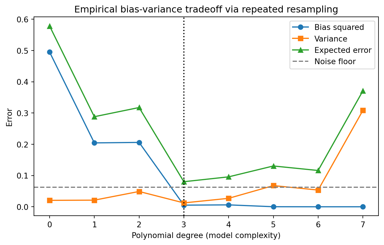
82.2.4 2.4 Measuring bias and variance empirically
The decomposition is not just a thought experiment. We can estimate bias squared and variance directly by Monte Carlo: draw many independent training sets, fit a model on each, and look at how the predictions behave across the ensemble at a fixed grid of test points. The average prediction estimates \(\bar{f}\), the squared gap from the truth estimates bias squared, and the spread of predictions estimates variance. The following panels show the same experiment in three languages. The Python panel is executable and produces the plot and table; the Julia and Rust panels are illustrative and mirror the same logic.
# Illustrative Julia: same Monte Carlo estimate of bias and variance.usingRandom, Statistics, Polynomialsf_true(x) =sin(2pi * x)sigma, n_train, n_datasets =0.25, 30, 200degrees =0:7x_test =range(0.0, 1.0; length =100)f_test =f_true.(x_test)for d in degrees rng =MersenneTwister(0) preds =Array{Float64}(undef, n_datasets, length(x_test))for k in1:n_datasets x_tr =rand(rng, n_train) y_tr =f_true.(x_tr) .+ sigma .*randn(rng, n_train) p =fit(Polynomial, x_tr, y_tr, d) # least-squares polynomial preds[k, :] =p.(x_test)end mean_pred =vec(mean(preds; dims =1)) bias2 =mean((mean_pred .- f_test) .^2) variance =mean(vec(var(preds; dims =1)))println("degree=$d bias2=$(round(bias2, digits=4)) var=$(round(variance, digits=4))")end
// Illustrative Rust: structure of the resampling loop (least-squares fit elided).// Run with a crate such as `nalgebra` for the polynomial regression solve.fn f_true(x:f64) ->f64{ (2.0*std::f64::consts::PI * x).sin()}fn main() {let sigma =0.25_f64;let n_train =30;let n_datasets =200;let x_test:Vec<f64>= (0..100).map(|i| i asf64/99.0).collect();let f_test:Vec<f64>= x_test.iter().map(|&x| f_true(x)).collect();for d in0..=7{// For each of n_datasets training sets:// 1. sample x_tr uniformly on [0, 1], y_tr = f_true(x_tr) + sigma * noise// 2. fit a degree-d polynomial by least squares// 3. evaluate the fit at every x_test point and store the row// Then aggregate across datasets:// mean_pred[j] = average prediction at x_test[j]// bias2 = mean over j of (mean_pred[j] - f_test[j])^2// variance = mean over j of variance of predictions at x_test[j]let _ = (sigma, n_train, n_datasets, d,&f_test);println!("degree={d}: estimate bias^2 and variance by resampling");}}
82.3 3. Underfitting and Overfitting
82.3.1 3.1 Two failure modes
Underfitting is the high-bias regime. The model is too simple to capture the underlying relationship, so both training and test error are high and close together. The diagnostic signature is a large training error that does not improve with more data, because the bottleneck is representational capacity, not sample size.
Overfitting is the high-variance regime. The model has enough flexibility to memorize peculiarities of the training set, so training error is low while test error remains high. The diagnostic signature is a wide generalization gap: excellent training performance paired with poor validation performance.
82.3.2 3.2 Diagnosing with learning curves
Learning curves plot error against training set size and are the workhorse diagnostic. In an underfitting model, training and validation error converge quickly to a high plateau. In an overfitting model, training error stays low while validation error sits well above it, and the gap shrinks slowly as data accumulates. This distinction drives the remedy: underfitting calls for a richer model or better features, while overfitting calls for more data, regularization, or a simpler model.
# Sketch of the diagnostic logic, not runnable production code
if train_error_high and gap_small:
    diagnosis = "underfitting (high bias): add capacity or features"
elif train_error_low and gap_large:
    diagnosis = "overfitting (high variance): regularize or add data"
else:
    diagnosis = "well balanced: error near the noise floor"
82.3.3 3.3 Regularization as a tradeoff knob
Regularization is the most direct instrument for tuning the balance. Ridge regression, for instance, minimizes
The penalty \(\lambda\) shrinks coefficients toward zero. As \(\lambda\) increases, the estimator becomes more constrained: variance falls because the fit is less sensitive to the particular sample, while bias rises because the model is pulled away from the unconstrained least-squares solution. The value \(\lambda = 0\) recovers ordinary least squares (low bias, high variance), and \(\lambda \to \infty\) forces the trivial zero predictor (high bias, zero variance). Cross-validation chooses the \(\lambda\) that minimizes estimated risk, which is precisely the point where the marginal decrease in variance no longer outweighs the marginal increase in bias.
Other mechanisms act through the same lens. Early stopping in iterative training limits how far parameters travel from their initialization, which behaves like an implicit penalty. Dropout and data augmentation inject controlled randomness that suppresses variance. Ensembling, especially bagging, averages many high-variance predictors to cancel their independent fluctuations while leaving bias roughly unchanged, which is why random forests work so well.
82.4 4. How Complexity and Data Size Shift the Tradeoff
82.4.1 4.1 The role of model complexity
Holding the dataset fixed and sweeping model complexity traces out the classical U-shaped risk curve. At low complexity, bias dominates and total error is high. As complexity grows, bias falls quickly while variance creeps up, and total error descends to a minimum. Past that minimum, variance grows faster than bias falls, and error climbs again. The minimum of this U is the classical notion of optimal capacity, and for decades it was treated as the final word.
We can make the U-shape precise. Let complexity be indexed by a scalar \(c\) (for polynomials, the degree \(d\)). Write the bias-squared and variance contributions, integrated over the input distribution, as functions of \(c\):
In the classical regime \(B(c)\) decreases and \(V(c)\) increases as \(c\) grows, so \(B'(c) < 0\) and \(V'(c) > 0\). The optimal complexity \(c^\star\) satisfies the first-order condition
so the minimum sits exactly where the marginal reduction in bias squared equals the marginal increase in variance. To the left of \(c^\star\) bias still falls faster than variance rises and we should add capacity; to the right the balance reverses. This is the formal content of the U-curve, and it explains why the noise floor \(\sigma^2\) shifts the whole curve up but never moves the location of \(c^\star\).
Complexity here is not just a count of parameters. It is better captured by effective capacity measures such as the Vapnik-Chervonenkis dimension or Rademacher complexity, which quantify how many distinct labelings a hypothesis class can realize. Two models with the same parameter count but different inductive biases can sit at very different points on the curve.
82.4.2 4.2 The role of dataset size
Now hold complexity fixed and grow \(n\). Variance generally shrinks as \(1/n\) in well-behaved estimators, because more data averages out sampling noise. Bias, by contrast, is largely insensitive to \(n\): it reflects the limits of the hypothesis class, and no amount of additional data lets a linear model bend into a curve. This asymmetry has a powerful consequence. With abundant data, the variance term is suppressed, which means you can afford a more complex, lower-bias model without paying a variance penalty. This is the statistical engine behind the success of large models in data-rich domains: scale neutralizes variance, so the dominant remaining error source is bias, and the way to reduce bias is to enlarge the hypothesis class.
82.4.3 4.3 The interaction
Complexity and data size therefore interact. The optimal complexity is an increasing function of \(n\). On a small dataset the U-curve minimum sits at a modest capacity; as \(n\) grows, the minimum slides rightward toward richer models. A useful mental model is the ratio of parameters to samples. When parameters are scarce relative to data, you live on the underfitting side and should add capacity. When parameters vastly exceed data, classical theory predicts ruinous variance. That prediction is exactly where the modern picture diverges from the classical one.
82.5 5. The Modern Double-Descent Picture
82.5.1 5.1 The interpolation threshold
Deep networks routinely have far more parameters than training examples, fit their training data to essentially zero error, and yet generalize well. Classical bias-variance reasoning says this should be impossible: a model flexible enough to interpolate noisy data should have catastrophic variance. The resolution is the double-descent phenomenon, characterized empirically and named by Belkin and collaborators in 2019, building on earlier observations.
The story extends the U-curve. As complexity increases toward the point where the model can exactly fit the training data, the interpolation threshold, test error does spike upward as the classical theory predicts. The number of parameters needed to interpolate roughly equals the number of training points, and right at that boundary the fit is maximally unstable. But as complexity increases past the threshold, test error descends a second time, often falling below the classical U-curve minimum.
test
error
  |        classical                modern
  |        U-curve                  regime
  |      __
  |     /  \      /\  <- spike at interpolation threshold
  |    /    \    /  \___
  |   /      \__/       \________  second descent
  |__/
  |________________________________ model complexity
                    ^
              interpolation
                threshold
82.5.2 5.2 Why the second descent happens
The intuition is that among the infinitely many models that perfectly interpolate the training data, the training procedure does not pick an arbitrary one. Gradient descent applied to overparameterized models exhibits an implicit bias toward low-norm, smooth solutions. When many interpolating solutions exist, the optimizer tends to find one with small parameter norm, which behaves like a regularized, low-variance estimator despite the enormous parameter count. Adding parameters past the threshold enlarges the space of interpolating solutions, giving the optimizer more room to find a smooth one, so the effective variance falls even as the nominal capacity rises.
This reframes the relationship between parameter count and the relevant notion of complexity. Raw parameter count is a poor proxy for capacity once implicit regularization is in play. The quantity that governs generalization is something closer to the norm of the solution the optimizer actually reaches, not the dimensionality of the space it could in principle explore.
82.5.3 5.3 Sample-wise and epoch-wise double descent
Double descent is not confined to model size. A sample-wise version appears when, counterintuitively, adding training data can temporarily increase test error if it pushes the system closer to its interpolation threshold for a fixed model size. An epoch-wise version appears during training itself, where test error can rise and then fall again as optimization proceeds. These variants share a common structure: error peaks when the effective capacity and the effective difficulty of the fitting problem are matched, and improves as the system moves away from that critical balance in either direction.
82.5.4 5.4 Reconciling classical and modern views
The two pictures are not in contradiction. The classical bias-variance decomposition remains exactly correct as an algebraic identity; it never stops being true that error equals bias squared plus variance plus noise. What changed is our understanding of how variance behaves for overparameterized models trained with implicit regularization. The classical analysis implicitly assumed that more parameters always means more variance. Modern practice shows that beyond the interpolation threshold, the implicit bias of the optimizer can drive variance back down. Double descent is therefore a refinement of the variance term, not a repeal of the decomposition.
For practitioners, the lesson is nuanced. In the classical underparameterized regime, the old advice holds: control complexity, regularize, and respect the U-curve. In the modern overparameterized regime, the productive moves are often to scale the model well past interpolation, lean on the optimizer’s implicit regularization, and add data and compute. The dangerous zone is the interpolation threshold itself, where models are large enough to memorize but not large enough to be smoothed by implicit bias. The standard remedies of explicit regularization and early stopping are most valuable precisely there.
82.6 6. Practical Synthesis
The bias-variance tradeoff endures as the conceptual backbone of generalization theory because it names the three sources of error and tells you which knobs move which term. Diagnose first: separate training error from the generalization gap to identify whether bias or variance dominates. If bias dominates, enrich the model, engineer better features, or, in the deep learning regime, scale up. If variance dominates, gather more data, regularize, ensemble, or simplify. Respect the noise floor so you do not waste effort chasing irreducible error. And when working with very large models, remember that parameter count alone no longer predicts variance: the optimizer’s implicit bias and the resulting solution norm are what govern generalization on the far side of the interpolation threshold. Holding both the classical and modern pictures in mind at once is what lets a practitioner reason correctly across the full range from a small regression model to a billion-parameter network.
82.7 References
Geman, S., Bienenstock, E., and Doursat, R. (1992). Neural Networks and the Bias/Variance Dilemma. Neural Computation. https://doi.org/10.1162/neco.1992.4.1.1
Hastie, T., Tibshirani, R., and Friedman, J. (2009). The Elements of Statistical Learning, 2nd ed. Springer. https://hastie.su.domains/ElemStatLearn/
Belkin, M., Hsu, D., Ma, S., and Mandal, S. (2019). Reconciling Modern Machine Learning Practice and the Classical Bias-Variance Trade-off. PNAS. https://doi.org/10.1073/pnas.1903070116
Nakkiran, P., Kaplun, G., Bansal, Y., Yang, T., Barak, B., and Sutskever, I. (2021). Deep Double Descent: Where Bigger Models and More Data Hurt. Journal of Statistical Mechanics. https://doi.org/10.1088/1742-5468/ac3a74
Zhang, C., Bengio, S., Hardt, M., Recht, B., and Vinyals, O. (2017). Understanding Deep Learning Requires Rethinking Generalization. ICLR. https://arxiv.org/abs/1611.03530
Bishop, C. M. (2006). Pattern Recognition and Machine Learning. Springer. https://www.microsoft.com/en-us/research/publication/pattern-recognition-machine-learning/
Domingos, P. (2000). A Unified Bias-Variance Decomposition. ICML. https://homes.cs.washington.edu/~pedrod/papers/mlc00a.pdf
Vapnik, V. N. (1998). Statistical Learning Theory. Wiley. https://www.wiley.com/en-us/Statistical+Learning+Theory-p-9780471030034
Source Code
# The Bias-Variance TradeoffEvery supervised learning system makes a silent promise: that what it learned from a finite training sample will generalize to data it has never seen. The bias-variance tradeoff is the classical framework for understanding when and why that promise is kept or broken. It explains why a model that memorizes its training data can fail catastrophically in production, why a model that is too rigid can never capture the signal, and why the sweet spot between these failure modes shifts as we change model complexity and dataset size. This chapter develops the decomposition of expected error from first principles, connects it to the practical phenomena of underfitting and overfitting, and then confronts the modern double-descent picture that complicates the classical story for overparameterized models such as deep networks.## 1. Setting Up the Problem### 1.1 The learning setupWe assume data are drawn from a fixed but unknown joint distribution $P(x, y)$ over inputs $x \in \mathcal{X}$ and targets $y \in \mathcal{Y}$. A learning algorithm observes a training set $\mathcal{D} = \{(x_i, y_i)\}_{i=1}^{n}$ of $n$ independent and identically distributed samples and produces a predictor $\hat{f}_{\mathcal{D}}: \mathcal{X} \to \mathcal{Y}$. The notation $\hat{f}_{\mathcal{D}}$ emphasizes that the learned function is itself a random object: change the training set, and you get a different predictor.The quantity we ultimately care about is the generalization error, also called the risk:$$R(\hat{f}_{\mathcal{D}}) = \mathbb{E}_{(x,y) \sim P}\big[ L(\hat{f}_{\mathcal{D}}(x), y) \big],$$where $L$ is a loss function. The training error, by contrast, averages the loss over only the observed sample. The gap between these two is the generalization gap, and most of the theory in this chapter is an attempt to anatomize it.### 1.2 The noise floorA central assumption is that even the best possible predictor cannot achieve zero error. We model the target as$$y = f(x) + \varepsilon, \qquad \mathbb{E}[\varepsilon] = 0, \quad \mathrm{Var}(\varepsilon) = \sigma^2,$$where $f(x) = \mathbb{E}[y \mid x]$ is the regression function and $\varepsilon$ is irreducible noise independent of $x$. No learning procedure can predict $\varepsilon$, because by construction it is uncorrelated with the inputs. The variance $\sigma^2$ therefore sets a hard floor on achievable error. Recognizing this floor matters in practice: a team chasing zero validation loss on inherently noisy labels is chasing a mirage.## 2. The Decomposition of Expected Error### 2.1 Deriving the decomposition for squared lossConsider the squared error loss and fix a single test point $x_0$. We want the expected error at $x_0$, where the expectation is taken over both the random noise in the test label and the randomness of the training set $\mathcal{D}$. Write $\hat{f} = \hat{f}_{\mathcal{D}}(x_0)$ for brevity and let $\bar{f}(x_0) = \mathbb{E}_{\mathcal{D}}[\hat{f}_{\mathcal{D}}(x_0)]$ denote the average prediction across all possible training sets.The expected squared error decomposes exactly:$$\mathbb{E}\big[(y - \hat{f})^2\big] = \underbrace{\big(\bar{f}(x_0) - f(x_0)\big)^2}_{\text{Bias}^2} + \underbrace{\mathbb{E}_{\mathcal{D}}\big[(\hat{f} - \bar{f}(x_0))^2\big]}_{\text{Variance}} + \underbrace{\sigma^2}_{\text{Noise}}.$$We now derive this identity in full. The test label at $x_0$ is $y = f(x_0) + \varepsilon$ with $\mathbb{E}[\varepsilon] = 0$ and $\mathrm{Var}(\varepsilon) = \sigma^2$, and $\varepsilon$ is independent of the training set $\mathcal{D}$. Start by inserting $f(x_0)$ and splitting the error into a noise part and a model part:$$y - \hat{f} = \big(f(x_0) + \varepsilon\big) - \hat{f} = \varepsilon + \big(f(x_0) - \hat{f}\big).$$Squaring and taking the expectation over both $\varepsilon$ and $\mathcal{D}$ gives$$\mathbb{E}\big[(y - \hat{f})^2\big] = \mathbb{E}[\varepsilon^2] + 2\,\mathbb{E}\big[\varepsilon\,(f(x_0) - \hat{f})\big] + \mathbb{E}\big[(f(x_0) - \hat{f})^2\big].$$The first term is $\mathbb{E}[\varepsilon^2] = \mathrm{Var}(\varepsilon) = \sigma^2$. The cross term vanishes because $\varepsilon$ is independent of $\hat{f}_{\mathcal{D}}$ and has zero mean, so $\mathbb{E}[\varepsilon\,(f(x_0) - \hat{f})] = \mathbb{E}[\varepsilon]\,\mathbb{E}[f(x_0) - \hat{f}] = 0$. We are left with the reducible error $\mathbb{E}[(f(x_0) - \hat{f})^2]$.Now apply the same add-and-subtract trick to the reducible error, this time centering on the average prediction $\bar{f}(x_0) = \mathbb{E}_{\mathcal{D}}[\hat{f}]$:$$f(x_0) - \hat{f} = \big(f(x_0) - \bar{f}(x_0)\big) + \big(\bar{f}(x_0) - \hat{f}\big).$$Squaring and taking the expectation over $\mathcal{D}$,$$\mathbb{E}_{\mathcal{D}}\big[(f(x_0) - \hat{f})^2\big] = \big(f(x_0) - \bar{f}(x_0)\big)^2 + 2\big(f(x_0) - \bar{f}(x_0)\big)\,\mathbb{E}_{\mathcal{D}}\big[\bar{f}(x_0) - \hat{f}\big] + \mathbb{E}_{\mathcal{D}}\big[(\bar{f}(x_0) - \hat{f})^2\big].$$The first term is deterministic and equals $\text{Bias}^2$. The cross term vanishes because $\mathbb{E}_{\mathcal{D}}[\bar{f}(x_0) - \hat{f}] = \bar{f}(x_0) - \mathbb{E}_{\mathcal{D}}[\hat{f}] = 0$ by definition of $\bar{f}(x_0)$. The last term is the variance $\mathbb{E}_{\mathcal{D}}[(\hat{f} - \bar{f}(x_0))^2]$. Collecting the surviving pieces reproduces the three-term identity above. The decomposition is exact: it is an algebraic rearrangement, not an approximation, and it holds for any predictor and any data distribution under squared loss.### 2.2 Reading the three termsEach term has a clean interpretation.**Bias** measures how far the average prediction is from the truth. It captures systematic error introduced by the modeling assumptions. A linear model fit to a quadratic signal has high bias no matter how much data you give it, because the hypothesis class simply cannot represent the curvature.**Variance** measures how much the prediction wobbles as the training set changes. A model with many degrees of freedom relative to the data will fit the idiosyncratic noise of each particular sample, so its predictions swing wildly from one draw to the next.**Noise** is the irreducible $\sigma^2$. It is a property of the data-generating process, not of the model, and it cannot be reduced by any choice of algorithm.The practical upshot is that total error is a sum of one term we cannot touch and two terms we trade against each other. The art of model selection is largely the art of navigating this tradeoff.### 2.3 A worked intuitionImagine fitting polynomials of degree $d$ to noisy samples from a smooth curve. With $d = 0$ (a constant), the fitted line ignores all structure: predictions barely change across training sets, so variance is tiny, but the constant is systematically wrong almost everywhere, so bias is large. With $d = 15$ and only twenty data points, the polynomial snakes through every point, including the noise. Across resamples the fitted curve is unrecognizable from one run to the next: variance dominates while bias is near zero. Somewhere in between, perhaps $d = 3$, the two contributions balance and total error is minimized.```texterror | \ / | \ total / | \___ ____/ | \___ ___/ variance | bias^2 \____/ |________________________________ model complexity underfit sweet overfit spot```### 2.4 Measuring bias and variance empiricallyThe decomposition is not just a thought experiment. We can estimate bias squared and variance directly by Monte Carlo: draw many independent training sets, fit a model on each, and look at how the predictions behave across the ensemble at a fixed grid of test points. The average prediction estimates $\bar{f}$, the squared gap from the truth estimates bias squared, and the spread of predictions estimates variance. The following panels show the same experiment in three languages. The Python panel is executable and produces the plot and table; the Julia and Rust panels are illustrative and mirror the same logic.::: {.panel-tabset}## Python```{python}import numpy as npimport matplotlib.pyplot as pltfrom sklearn.preprocessing import PolynomialFeaturesfrom sklearn.linear_model import LinearRegressionfrom sklearn.pipeline import make_pipelinerng = np.random.default_rng(0)def f_true(x):return np.sin(2.0* np.pi * x)sigma =0.25# irreducible noise standard deviationn_train =30# training points per resampled datasetn_datasets =200# number of independent training setsdegrees =list(range(0, 8)) # polynomial degrees to sweepx_test = np.linspace(0.0, 1.0, 100)f_test = f_true(x_test)bias2_by_degree, var_by_degree, err_by_degree = [], [], []for d in degrees: preds = np.empty((n_datasets, x_test.size))for k inrange(n_datasets): x_tr = rng.uniform(0.0, 1.0, size=n_train) y_tr = f_true(x_tr) + rng.normal(0.0, sigma, size=n_train) model = make_pipeline(PolynomialFeatures(degree=d), LinearRegression()) model.fit(x_tr.reshape(-1, 1), y_tr) preds[k] = model.predict(x_test.reshape(-1, 1)) mean_pred = preds.mean(axis=0) bias2 =float(np.mean((mean_pred - f_test) **2)) variance =float(np.mean(preds.var(axis=0))) bias2_by_degree.append(bias2) var_by_degree.append(variance) err_by_degree.append(bias2 + variance + sigma **2)best =int(np.argmin(err_by_degree))print("degree | bias^2 | variance | expected_err")for d, b, v, e inzip(degrees, bias2_by_degree, var_by_degree, err_by_degree):print(f"{d:6d} | {b:6.4f} | {v:8.4f} | {e:12.4f}")print(f"\nNoise floor sigma^2 = {sigma**2:.4f}")print(f"Minimum expected error at degree {degrees[best]}")fig, ax = plt.subplots(figsize=(7, 4.5))ax.plot(degrees, bias2_by_degree, marker="o", label="Bias squared")ax.plot(degrees, var_by_degree, marker="s", label="Variance")ax.plot(degrees, err_by_degree, marker="^", label="Expected error")ax.axhline(sigma **2, linestyle="--", color="gray", label="Noise floor")ax.axvline(degrees[best], linestyle=":", color="black")ax.set_xlabel("Polynomial degree (model complexity)")ax.set_ylabel("Error")ax.set_title("Empirical bias-variance tradeoff via repeated resampling")ax.legend()fig.tight_layout()plt.show()```## Julia```julia# Illustrative Julia: same Monte Carlo estimate of bias and variance.usingRandom, Statistics, Polynomialsf_true(x) =sin(2pi * x)sigma, n_train, n_datasets =0.25, 30, 200degrees =0:7x_test =range(0.0, 1.0; length =100)f_test =f_true.(x_test)for d in degrees rng =MersenneTwister(0) preds =Array{Float64}(undef, n_datasets, length(x_test))for k in1:n_datasets x_tr =rand(rng, n_train) y_tr =f_true.(x_tr) .+ sigma .*randn(rng, n_train) p =fit(Polynomial, x_tr, y_tr, d) # least-squares polynomial preds[k, :] =p.(x_test)end mean_pred =vec(mean(preds; dims =1)) bias2 =mean((mean_pred .- f_test) .^2) variance =mean(vec(var(preds; dims =1)))println("degree=$d bias2=$(round(bias2, digits=4)) var=$(round(variance, digits=4))")end```## Rust```rust// Illustrative Rust: structure of the resampling loop (least-squares fit elided).// Run with a crate such as `nalgebra`for the polynomial regression solve.fn f_true(x: f64) -> f64 { (2.0* std::f64::consts::PI * x).sin()}fn main() { let sigma =0.25_f64; let n_train =30; let n_datasets =200; let x_test: Vec<f64>= (0..100).map(|i| i as f64 /99.0).collect(); let f_test: Vec<f64>=x_test.iter().map(|&x|f_true(x)).collect();for d in0..=7 {// For each of n_datasets training sets://1. sample x_tr uniformly on [0, 1], y_tr =f_true(x_tr) + sigma * noise//2. fit a degree-d polynomial by least squares//3. evaluate the fit at every x_test point and store the row// Then aggregate across datasets:// mean_pred[j] = average prediction at x_test[j]// bias2 = mean over j of (mean_pred[j] - f_test[j])^2// variance = mean over j of variance of predictions at x_test[j] let _ = (sigma, n_train, n_datasets, d, &f_test); println!("degree={d}: estimate bias^2 and variance by resampling"); }}```:::## 3. Underfitting and Overfitting### 3.1 Two failure modesUnderfitting is the high-bias regime. The model is too simple to capture the underlying relationship, so both training and test error are high and close together. The diagnostic signature is a large training error that does not improve with more data, because the bottleneck is representational capacity, not sample size.Overfitting is the high-variance regime. The model has enough flexibility to memorize peculiarities of the training set, so training error is low while test error remains high. The diagnostic signature is a wide generalization gap: excellent training performance paired with poor validation performance.### 3.2 Diagnosing with learning curvesLearning curves plot error against training set size and are the workhorse diagnostic. In an underfitting model, training and validation error converge quickly to a high plateau. In an overfitting model, training error stays low while validation error sits well above it, and the gap shrinks slowly as data accumulates. This distinction drives the remedy: underfitting calls for a richer model or better features, while overfitting calls for more data, regularization, or a simpler model.```text# Sketch of the diagnostic logic, not runnable production codeif train_error_high and gap_small: diagnosis = "underfitting (high bias): add capacity or features"elif train_error_low and gap_large: diagnosis = "overfitting (high variance): regularize or add data"else: diagnosis = "well balanced: error near the noise floor"```### 3.3 Regularization as a tradeoff knobRegularization is the most direct instrument for tuning the balance. Ridge regression, for instance, minimizes$$\hat{\beta} = \arg\min_{\beta} \; \|y - X\beta\|_2^2 + \lambda \|\beta\|_2^2.$$The penalty $\lambda$ shrinks coefficients toward zero. As $\lambda$ increases, the estimator becomes more constrained: variance falls because the fit is less sensitive to the particular sample, while bias rises because the model is pulled away from the unconstrained least-squares solution. The value $\lambda = 0$ recovers ordinary least squares (low bias, high variance), and $\lambda \to \infty$ forces the trivial zero predictor (high bias, zero variance). Cross-validation chooses the $\lambda$ that minimizes estimated risk, which is precisely the point where the marginal decrease in variance no longer outweighs the marginal increase in bias.Other mechanisms act through the same lens. Early stopping in iterative training limits how far parameters travel from their initialization, which behaves like an implicit penalty. Dropout and data augmentation inject controlled randomness that suppresses variance. Ensembling, especially bagging, averages many high-variance predictors to cancel their independent fluctuations while leaving bias roughly unchanged, which is why random forests work so well.## 4. How Complexity and Data Size Shift the Tradeoff### 4.1 The role of model complexityHolding the dataset fixed and sweeping model complexity traces out the classical U-shaped risk curve. At low complexity, bias dominates and total error is high. As complexity grows, bias falls quickly while variance creeps up, and total error descends to a minimum. Past that minimum, variance grows faster than bias falls, and error climbs again. The minimum of this U is the classical notion of optimal capacity, and for decades it was treated as the final word.We can make the U-shape precise. Let complexity be indexed by a scalar $c$ (for polynomials, the degree $d$). Write the bias-squared and variance contributions, integrated over the input distribution, as functions of $c$:$$\mathrm{Err}(c) = B(c) + V(c) + \sigma^2, \qquad B(c) = \mathbb{E}_{x}\big[(\bar{f}_c(x) - f(x))^2\big], \quad V(c) = \mathbb{E}_{x}\,\mathbb{E}_{\mathcal{D}}\big[(\hat{f}_{c,\mathcal{D}}(x) - \bar{f}_c(x))^2\big].$$In the classical regime $B(c)$ decreases and $V(c)$ increases as $c$ grows, so $B'(c) < 0$ and $V'(c) > 0$. The optimal complexity $c^\star$ satisfies the first-order condition$$\frac{d\,\mathrm{Err}}{dc}\bigg|_{c^\star} = B'(c^\star) + V'(c^\star) = 0 \quad\Longrightarrow\quad B'(c^\star) = -V'(c^\star),$$so the minimum sits exactly where the marginal reduction in bias squared equals the marginal increase in variance. To the left of $c^\star$ bias still falls faster than variance rises and we should add capacity; to the right the balance reverses. This is the formal content of the U-curve, and it explains why the noise floor $\sigma^2$ shifts the whole curve up but never moves the location of $c^\star$.Complexity here is not just a count of parameters. It is better captured by effective capacity measures such as the Vapnik-Chervonenkis dimension or Rademacher complexity, which quantify how many distinct labelings a hypothesis class can realize. Two models with the same parameter count but different inductive biases can sit at very different points on the curve.### 4.2 The role of dataset sizeNow hold complexity fixed and grow $n$. Variance generally shrinks as $1/n$ in well-behaved estimators, because more data averages out sampling noise. Bias, by contrast, is largely insensitive to $n$: it reflects the limits of the hypothesis class, and no amount of additional data lets a linear model bend into a curve. This asymmetry has a powerful consequence. With abundant data, the variance term is suppressed, which means you can afford a more complex, lower-bias model without paying a variance penalty. This is the statistical engine behind the success of large models in data-rich domains: scale neutralizes variance, so the dominant remaining error source is bias, and the way to reduce bias is to enlarge the hypothesis class.### 4.3 The interactionComplexity and data size therefore interact. The optimal complexity is an increasing function of $n$. On a small dataset the U-curve minimum sits at a modest capacity; as $n$ grows, the minimum slides rightward toward richer models. A useful mental model is the ratio of parameters to samples. When parameters are scarce relative to data, you live on the underfitting side and should add capacity. When parameters vastly exceed data, classical theory predicts ruinous variance. That prediction is exactly where the modern picture diverges from the classical one.## 5. The Modern Double-Descent Picture### 5.1 The interpolation thresholdDeep networks routinely have far more parameters than training examples, fit their training data to essentially zero error, and yet generalize well. Classical bias-variance reasoning says this should be impossible: a model flexible enough to interpolate noisy data should have catastrophic variance. The resolution is the double-descent phenomenon, characterized empirically and named by Belkin and collaborators in 2019, building on earlier observations.The story extends the U-curve. As complexity increases toward the point where the model can exactly fit the training data, the interpolation threshold, test error does spike upward as the classical theory predicts. The number of parameters needed to interpolate roughly equals the number of training points, and right at that boundary the fit is maximally unstable. But as complexity increases past the threshold, test error descends a second time, often falling below the classical U-curve minimum.```texttesterror | classical modern | U-curve regime | __ | / \ /\ <- spike at interpolation threshold | / \ / \___ | / \__/ \________ second descent |__/ |________________________________ model complexity ^ interpolation threshold```### 5.2 Why the second descent happensThe intuition is that among the infinitely many models that perfectly interpolate the training data, the training procedure does not pick an arbitrary one. Gradient descent applied to overparameterized models exhibits an implicit bias toward low-norm, smooth solutions. When many interpolating solutions exist, the optimizer tends to find one with small parameter norm, which behaves like a regularized, low-variance estimator despite the enormous parameter count. Adding parameters past the threshold enlarges the space of interpolating solutions, giving the optimizer more room to find a smooth one, so the effective variance falls even as the nominal capacity rises.This reframes the relationship between parameter count and the relevant notion of complexity. Raw parameter count is a poor proxy for capacity once implicit regularization is in play. The quantity that governs generalization is something closer to the norm of the solution the optimizer actually reaches, not the dimensionality of the space it could in principle explore.### 5.3 Sample-wise and epoch-wise double descentDouble descent is not confined to model size. A sample-wise version appears when, counterintuitively, adding training data can temporarily increase test error if it pushes the system closer to its interpolation threshold for a fixed model size. An epoch-wise version appears during training itself, where test error can rise and then fall again as optimization proceeds. These variants share a common structure: error peaks when the effective capacity and the effective difficulty of the fitting problem are matched, and improves as the system moves away from that critical balance in either direction.### 5.4 Reconciling classical and modern viewsThe two pictures are not in contradiction. The classical bias-variance decomposition remains exactly correct as an algebraic identity; it never stops being true that error equals bias squared plus variance plus noise. What changed is our understanding of how variance behaves for overparameterized models trained with implicit regularization. The classical analysis implicitly assumed that more parameters always means more variance. Modern practice shows that beyond the interpolation threshold, the implicit bias of the optimizer can drive variance back down. Double descent is therefore a refinement of the variance term, not a repeal of the decomposition.For practitioners, the lesson is nuanced. In the classical underparameterized regime, the old advice holds: control complexity, regularize, and respect the U-curve. In the modern overparameterized regime, the productive moves are often to scale the model well past interpolation, lean on the optimizer's implicit regularization, and add data and compute. The dangerous zone is the interpolation threshold itself, where models are large enough to memorize but not large enough to be smoothed by implicit bias. The standard remedies of explicit regularization and early stopping are most valuable precisely there.## 6. Practical SynthesisThe bias-variance tradeoff endures as the conceptual backbone of generalization theory because it names the three sources of error and tells you which knobs move which term. Diagnose first: separate training error from the generalization gap to identify whether bias or variance dominates. If bias dominates, enrich the model, engineer better features, or, in the deep learning regime, scale up. If variance dominates, gather more data, regularize, ensemble, or simplify. Respect the noise floor so you do not waste effort chasing irreducible error. And when working with very large models, remember that parameter count alone no longer predicts variance: the optimizer's implicit bias and the resulting solution norm are what govern generalization on the far side of the interpolation threshold. Holding both the classical and modern pictures in mind at once is what lets a practitioner reason correctly across the full range from a small regression model to a billion-parameter network.## References1. Geman, S., Bienenstock, E., and Doursat, R. (1992). Neural Networks and the Bias/Variance Dilemma. Neural Computation. https://doi.org/10.1162/neco.1992.4.1.12. Hastie, T., Tibshirani, R., and Friedman, J. (2009). The Elements of Statistical Learning, 2nd ed. Springer. https://hastie.su.domains/ElemStatLearn/3. Belkin, M., Hsu, D., Ma, S., and Mandal, S. (2019). Reconciling Modern Machine Learning Practice and the Classical Bias-Variance Trade-off. PNAS. https://doi.org/10.1073/pnas.19030701164. Nakkiran, P., Kaplun, G., Bansal, Y., Yang, T., Barak, B., and Sutskever, I. (2021). Deep Double Descent: Where Bigger Models and More Data Hurt. Journal of Statistical Mechanics. https://doi.org/10.1088/1742-5468/ac3a745. Zhang, C., Bengio, S., Hardt, M., Recht, B., and Vinyals, O. (2017). Understanding Deep Learning Requires Rethinking Generalization. ICLR. https://arxiv.org/abs/1611.035306. Bishop, C. M. (2006). Pattern Recognition and Machine Learning. Springer. https://www.microsoft.com/en-us/research/publication/pattern-recognition-machine-learning/7. Domingos, P. (2000). A Unified Bias-Variance Decomposition. ICML. https://homes.cs.washington.edu/~pedrod/papers/mlc00a.pdf8. Vapnik, V. N. (1998). Statistical Learning Theory. Wiley. https://www.wiley.com/en-us/Statistical+Learning+Theory-p-9780471030034