Linear algebra is the language in which modern machine learning is written. Every forward pass through a neural network, every attention computation in a transformer, and every gradient update during training reduces to a sequence of matrix operations. This chapter develops matrices not as grids of numbers to be manipulated by rote, but as concrete representations of linear maps between vector spaces. We then connect each concept (multiplication, transpose, inverse, rank, determinant, block structure) to how it actually appears inside machine learning systems, where these operations run thousands of times per second across batched tensors on specialized hardware.
23.1 1. Matrices as Linear Maps
The most important idea in this chapter is that a matrix is a function. Specifically, an \(m \times n\) matrix \(A\) represents a linear map \(T : \mathbb{R}^n \to \mathbb{R}^m\) that takes a vector in \(n\)-dimensional space and produces a vector in \(m\)-dimensional space.
23.1.1 1.1 What Linearity Means
A map \(T\) is linear when it respects vector addition and scalar multiplication:
for all vectors \(x, y\) and scalars \(\alpha, \beta\). This single property has a powerful consequence: a linear map is completely determined by what it does to a basis. If we know where each standard basis vector \(e_j = (0, \ldots, 1, \ldots, 0)^\top\) lands, we know where every vector lands, because any vector is a linear combination of basis vectors.
Suppose \(T(e_j) = a_j\), the \(j\)-th column of our matrix. Then for \(x = \sum_j x_j e_j\),
This is exactly the matrix-vector product \(Ax\). The columns of \(A\) are the images of the basis vectors, and \(Ax\) forms a linear combination of those columns weighted by the entries of \(x\).
23.1.2 1.2 The Column Picture
This column picture is the single most useful mental model for machine learning practitioners. Reading \(Ax\) as a weighted sum of columns explains, for example, why a linear layer with weight matrix \(W\) produces outputs that live in the span of \(W\)’s columns. The output space the model can reach is exactly the column space.
A neural network’s expressive power, before nonlinearities are added, is bounded by which directions its weight matrices can produce. Stacking linear maps without nonlinear activations collapses to a single linear map, which is why activation functions are essential: they break the chain of pure linearity that would otherwise make depth pointless.
23.2 2. Matrix Multiplication and Its Meaning
If matrices are linear maps, then matrix multiplication is composition of maps. Given \(B : \mathbb{R}^p \to \mathbb{R}^n\) and \(A : \mathbb{R}^n \to \mathbb{R}^m\), the composite \(A \circ B\) first applies \(B\), then \(A\), giving a map \(\mathbb{R}^p \to \mathbb{R}^m\). The matrix of this composite is the product \(AB\).
23.2.1 2.1 The Definition Follows from Composition
We do not invent the multiplication rule arbitrarily. We derive it by requiring \((AB)x = A(Bx)\) for every \(x\). Write \(B\) in terms of its columns and let \(x = e_k\), the \(k\)-th standard basis vector. Then \(Bx = B e_k\) is the \(k\)-th column of \(B\), whose \(j\)-th entry is \(B_{jk}\). Applying \(A\) gives
\[A(B e_k) = A \sum_{j=1}^{n} B_{jk}\, e_j^{(n)} = \sum_{j=1}^{n} B_{jk}\, (A e_j^{(n)}),\]
where \(A e_j^{(n)}\) is the \(j\)-th column of \(A\), whose \(i\)-th entry is \(A_{ij}\). Reading off the \(i\)-th entry of the result,
This formula is forced on us: it is the only rule consistent with composition. The entry in row \(i\), column \(k\) of the product is the dot product of row \(i\) of \(A\) with column \(k\) of \(B\). For this to be defined, the inner dimensions must match: \(A\) is \(m \times n\) and \(B\) is \(n \times p\), producing an \(m \times p\) result. Associativity \((AB)C = A(BC)\) is then immediate, because composition of functions is associative: both sides send \(x\) to the same vector \(A(B(Cx))\).
23.2.2 2.2 Multiple Ways to Read a Product
Matrix multiplication can be read at several levels, and fluency means switching between them freely:
Entry view: each output entry is a dot product (the formula above).
Column view: column \(k\) of \(AB\) equals \(A\) applied to column \(k\) of \(B\). The product transforms each column of \(B\).
Row view: row \(i\) of \(AB\) equals row \(i\) of \(A\) times \(B\).
Outer-product view: \(AB = \sum_{j} (\text{col}_j A)(\text{row}_j B)\), a sum of rank-one matrices.
The outer-product view is especially valuable in machine learning. Low-rank adaptation methods such as LoRA exploit exactly this decomposition, representing a weight update as a sum of a few outer products rather than a full dense matrix, which dramatically reduces the number of trainable parameters.
23.2.3 2.3 Properties and Costs
Matrix multiplication is associative, \((AB)C = A(BC)\), and distributive over addition, but it is not commutative: \(AB \neq BA\) in general. Associativity matters for efficiency. Computing \(A(BC)\) versus \((AB)C\) can differ enormously in cost depending on the shapes involved, a fact compilers exploit when optimizing computation graphs.
The naive cost of multiplying an \(m \times n\) by an \(n \times p\) matrix is \(O(mnp)\) scalar multiply-add operations. Because so much of training time is spent here, hardware accelerators (GPUs and TPUs) are designed around dense matrix multiplication, and a great deal of systems engineering goes into keeping these units busy.
23.3 3. Transpose
The transpose \(A^\top\) flips a matrix across its diagonal: \((A^\top)_{ij} = A_{ji}\). An \(m \times n\) matrix becomes \(n \times m\).
23.3.1 3.1 The Adjoint Interpretation
The transpose is not merely a bookkeeping operation. It is the adjoint of the linear map with respect to the standard inner product. Concretely, for all vectors \(x\) and \(y\),
\[\langle Ax, y \rangle = \langle x, A^\top y \rangle.\]
This is a short computation. With \(\langle u, v \rangle = \sum_i u_i v_i\),
where the middle step just reorders a finite double sum and recognizes \(\sum_i A_{ij} y_i = (A^\top y)_j\). The adjoint property characterizes the transpose uniquely: any matrix \(M\) satisfying \(\langle Ax, y \rangle = \langle x, My \rangle\) for all \(x, y\) must equal \(A^\top\).
This identity is the engine behind backpropagation. When a linear layer computes \(z = Wx\) in the forward pass, the gradient of the loss with respect to the input is obtained by applying \(W^\top\) to the upstream gradient:
So the forward pass uses \(W\) and the backward pass uses \(W^\top\). Every autodiff framework implements this transpose-multiply as the backward rule for a linear layer, which is why the transpose appears constantly in derivations of training algorithms.
23.3.2 3.2 Useful Identities
Two identities recur often. The transpose of a product reverses the order,
\[(AB)^\top = B^\top A^\top.\]
We can prove this directly from the entry formula. The \((i,k)\) entry of \((AB)^\top\) is the \((k,i)\) entry of \(AB\), namely \(\sum_j A_{kj} B_{ji}\). The \((i,k)\) entry of \(B^\top A^\top\) is \(\sum_j (B^\top)_{ij}(A^\top)_{jk} = \sum_j B_{ji} A_{kj}\), which is the same sum. The adjoint viewpoint gives the same result without indices: \(\langle ABx, y\rangle = \langle Bx, A^\top y\rangle = \langle x, B^\top A^\top y\rangle\), so the adjoint of \(AB\) is \(B^\top A^\top\).
A matrix satisfying \(A = A^\top\) is called symmetric. Symmetric matrices, particularly those of the form \(A^\top A\) (Gram matrices), appear throughout machine learning in covariance estimation, kernel methods, and the normal equations of least squares.
23.4 4. Identity and Inverse
23.4.1 4.1 The Identity
The identity matrix \(I_n\) is the matrix of the identity map: \(I_n x = x\) for every \(x\). It has ones on the diagonal and zeros elsewhere, and it acts as the multiplicative neutral element, \(AI = A\) and \(IA = A\). In residual networks, the skip connection \(y = x + F(x)\) can be read as \((I + F)\) applied to the input, and this identity term is what allows gradients to flow cleanly through very deep networks.
23.4.2 4.2 The Inverse
A square matrix \(A\) is invertible if there exists \(A^{-1}\) with
\[A A^{-1} = A^{-1} A = I.\]
The inverse represents the map that undoes \(A\). It exists exactly when \(A\) represents a bijection, meaning the linear map loses no information. Equivalently, \(A\) is invertible if and only if its columns are linearly independent, its determinant is nonzero, and its rank equals its dimension.
The inverse of a product reverses order, mirroring the transpose:
\[(AB)^{-1} = B^{-1} A^{-1}.\]
The proof is to verify the defining property. Using associativity,
\[(AB)(B^{-1} A^{-1}) = A(B B^{-1})A^{-1} = A I A^{-1} = A A^{-1} = I,\]
and symmetrically \((B^{-1} A^{-1})(AB) = I\). Since a two-sided inverse is unique (if \(CA = I = AD\) then \(C = C(AD) = (CA)D = D\)), the matrix \(B^{-1} A^{-1}\) is exactly \((AB)^{-1}\). A companion identity ties the inverse to the transpose: \((A^\top)^{-1} = (A^{-1})^\top\), because \(A^\top (A^{-1})^\top = (A^{-1} A)^\top = I^\top = I\).
23.4.3 4.3 Why We Rarely Compute Inverses
In numerical machine learning, explicitly forming \(A^{-1}\) is usually a mistake. Solving the linear system \(Ax = b\) directly (for example by LU or Cholesky factorization) is faster and far more numerically stable than computing \(A^{-1}\) and then multiplying. The conditioning of \(A\) governs how much small perturbations in \(b\) get amplified in the solution, and a poorly conditioned matrix can make naive inversion catastrophically inaccurate.
# Prefer this:
x = solve(A, b)          # factor once, solve
# Over this:
x = inverse(A) @ b       # slower, less stable
This principle carries into second-order optimization. Methods like Newton’s method conceptually require the inverse Hessian, but practical implementations solve a linear system or approximate the inverse rather than forming it explicitly.
23.5 5. Rank and Nullspace
Rank and nullspace describe how much a linear map compresses or preserves information.
23.5.1 5.1 The Four Fundamental Subspaces
Every \(m \times n\) matrix \(A\) defines four subspaces. The column space (range) is the set of all outputs \(Ax\), living in \(\mathbb{R}^m\). The nullspace (kernel) is the set of inputs that map to zero,
The row space and the left nullspace complete the picture, defined symmetrically from \(A^\top\). The rank is the dimension of the column space, equivalently the number of linearly independent columns (which always equals the number of linearly independent rows).
23.5.2 5.2 The Rank-Nullity Theorem
These dimensions are tied together by the rank-nullity theorem:
\[\text{rank}(A) + \dim(\text{null}(A)) = n,\]
where \(n\) is the number of columns. The idea behind the proof is a basis-extension argument. Suppose the nullspace has dimension \(k\) with basis \(\{u_1, \ldots, u_k\}\). Extend it to a basis of all of \(\mathbb{R}^n\) by adding vectors \(\{v_1, \ldots, v_{n-k}\}\). One then shows that the images \(\{Av_1, \ldots, Av_{n-k}\}\) form a basis of the column space: they span it because the \(u_i\) contribute nothing (they map to zero), and they are linearly independent because any dependence among the \(Av_j\) would force a combination of the \(v_j\) into the nullspace, contradicting that the \(v_j\) were chosen outside it. Hence \(\text{rank}(A) = n - k\), which rearranges to the theorem. Intuitively, each input dimension either contributes to a distinct output direction (counted in the rank) or gets crushed to zero (counted in the nullspace dimension). The map cannot do both with the same dimension.
23.5.3 5.3 Rank in Machine Learning
Rank is central to modern model design. A linear layer with a low-rank weight matrix has limited capacity to mix its inputs, since it can only produce outputs in a low-dimensional column space. This is sometimes a limitation and sometimes a deliberate efficiency choice.
Parameter-efficient fine-tuning is the clearest example. LoRA freezes a large pretrained weight matrix \(W_0\) and learns a low-rank update \(\Delta W = BA\), where \(B\) is \(d \times r\) and \(A\) is \(r \times d\) with \(r \ll d\). Because the update has rank at most \(r\), it requires only \(2dr\) parameters instead of \(d^2\), yet it captures most of the adaptation needed for a downstream task. The empirical success of LoRA suggests that the useful changes to a pretrained model often live in a low-rank subspace.
Rank deficiency also signals redundancy. If a feature matrix has rank below its column count, some features are linear combinations of others, the columns are collinear, and the least-squares solution is not unique. Regularization (ridge, for instance) restores a unique solution by effectively raising the rank of the system being solved.
23.6 6. Trace and Determinant
Two scalar functions summarize a square matrix in different ways.
23.6.1 6.1 Trace
The trace is the sum of diagonal entries,
\[\text{tr}(A) = \sum_{i} A_{ii}.\]
Its most useful property is cyclic invariance: \(\text{tr}(ABC) = \text{tr}(BCA) = \text{tr}(CAB)\), and in particular \(\text{tr}(AB) = \text{tr}(BA)\) even when \(AB\) and \(BA\) have different sizes. The base case is a one-line computation. For \(A\) of shape \(m \times n\) and \(B\) of shape \(n \times m\),
where the only move is swapping the order of a finite double sum. The three-factor cyclic identity follows by grouping: \(\text{tr}((AB)C) = \text{tr}(C(AB)) = \text{tr}((CA)B) = \text{tr}(B(CA))\). The trace also equals the sum of eigenvalues, which connects it to the total variance captured by a covariance matrix.
The trace shows up constantly in machine learning derivations. The squared Frobenius norm of a matrix is \(\|A\|_F^2 = \text{tr}(A^\top A)\), and many gradient identities are cleanest when expressed through the trace. The cyclic property is what lets us rearrange terms to extract gradients in matrix calculus.
23.6.2 6.2 Determinant
The determinant \(\det(A)\) measures how the linear map scales volume. If you apply \(A\) to a unit cube, the image is a parallelepiped whose signed volume is \(\det(A)\). A determinant of zero means the map flattens space into a lower dimension, which is exactly the condition for non-invertibility. A negative determinant indicates the map reverses orientation.
The determinant is multiplicative,
\[\det(AB) = \det(A)\det(B),\]
which follows from the volume-scaling interpretation: applying \(B\) then \(A\) scales volume by \(\det(B)\) and then by \(\det(A)\), so the composite scales by the product. Two consequences are immediate. First, if \(A\) is invertible then \(\det(A)\det(A^{-1}) = \det(A A^{-1}) = \det(I) = 1\), so \(\det(A^{-1}) = 1/\det(A)\), confirming that an invertible matrix has nonzero determinant. Second, the determinant equals the product of eigenvalues, so a zero eigenvalue (a nontrivial nullspace direction) forces \(\det(A) = 0\). In machine learning, the determinant appears most prominently in normalizing flows, a class of generative models that transform a simple base distribution through invertible maps. The change-of-variables formula requires the log absolute determinant of the Jacobian,
so flow architectures are deliberately designed (with triangular or coupling structures) to make this determinant cheap to compute. It also appears in the log-likelihood of a multivariate Gaussian, where the term \(\log\det(\Sigma)\) penalizes overly spread-out covariance estimates.
23.7 7. Block Matrices
Large matrices in practice are rarely treated as undifferentiated grids. They are organized into blocks, submatrices that can themselves be manipulated as units.
23.7.1 7.1 Block Operations
A block matrix partitions rows and columns into groups. When the partitions are compatible, multiplication works at the block level exactly as it does at the scalar level:
\[\begin{bmatrix} A & B \\ C & D \end{bmatrix} \begin{bmatrix} E & F \\ G & H \end{bmatrix} = \begin{bmatrix} AE + BG & AF + BH \\ CE + DG & CF + DH \end{bmatrix}.\]
This is more than notation. Treating blocks as units is how high-performance libraries tile matrix multiplication to fit cache and memory hierarchies, processing one block at a time so that data stays in fast memory while it is reused.
23.7.2 7.2 Block Structure in Models
Block thinking pervades model architecture. A transformer computes queries, keys, and values by projecting the input through three weight matrices that are often concatenated into a single block matrix \(W_{qkv} = [W_q \mid W_k \mid W_v]\) and applied in one fused operation, then split. Multi-head attention partitions the embedding dimension into blocks, one per head, each attending independently before the results are concatenated.
Block-diagonal matrices, where off-diagonal blocks are zero, represent maps that act independently on separate groups of coordinates. Grouped convolutions and mixture-of-experts routing both have this flavor: different parts of the input are processed by different parameter blocks, which saves computation and can be parallelized across devices.
23.8 8. Batched Operations in Machine Learning
Everything above describes single matrices acting on single vectors. Real machine learning systems operate on batches, and understanding the batch dimension is essential to reading model code and reasoning about performance.
23.8.1 8.1 The Linear Layer
A linear (fully connected) layer applies an affine map \(y = Wx + b\). With weight matrix \(W\) of shape \(m \times n\), it sends an \(n\)-dimensional input to an \(m\)-dimensional output. But we almost never feed one example at a time. Instead we stack \(B\) examples into a matrix \(X\) of shape \(B \times n\), one example per row, and compute
\[Y = X W^\top + b,\]
where \(Y\) has shape \(B \times m\) and the bias \(b\) is broadcast across rows. The transpose appears because of the row-major convention: with examples as rows, applying the map to every row at once is a single matrix multiplication. This one operation processes the entire batch, and it maps directly onto the matrix-multiply units of a GPU, which is why batching is the foundation of efficient training and inference.
23.8.2 8.2 Batched Matrix Multiplication
Beyond stacking vectors, modern architectures multiply stacks of matrices. A batched matrix multiply (often called bmm) takes two tensors of shape \(B \times n \times p\) and \(B \times p \times q\) and produces \(B \times n \times q\), performing \(B\) independent matrix products in parallel:
\[Z_b = X_b\, Y_b, \qquad b = 1, \ldots, B.\]
The leading dimension (sometimes several leading dimensions) is treated as a batch over which the same operation runs independently. Attention is the canonical consumer. For each example and each head, the scores are computed as
\[\text{scores} = \frac{Q K^\top}{\sqrt{d_k}},\]
where \(Q\) and \(K\) are matrices of shape (sequence length) by (head dimension), and this product is batched over both the example index and the head index. The softmax-weighted combination with the value matrix \(V\) is another batched product. A single attention layer therefore issues a large collection of small matrix multiplications, all dispatched together.
23.8.3 8.3 Broadcasting and Shape Discipline
Batched code relies on broadcasting, the rule by which arrays of different but compatible shapes are aligned by implicitly repeating along size-one dimensions. Adding a bias vector of shape \(m\) to an output of shape \(B \times m\) works because the bias is broadcast across the batch. Getting these shapes right is a large part of practical machine learning engineering, and shape mismatches are among the most common bugs.
# Conceptual shapes in an attention layer
Q, K, V : (B, heads, seq, d_head)
scores  = Q @ K.transpose(-2, -1)   # (B, heads, seq, seq)
attn    = softmax(scores / sqrt(d_head))
out     = attn @ V                  # (B, heads, seq, d_head)
23.8.4 8.4 Why This Framing Matters
Seeing these operations as batched linear algebra, rather than as opaque library calls, pays off in several ways. It clarifies where the computation actually goes, since the bulk of training time lives in a handful of large matrix multiplications. It explains memory cost, since intermediate tensors like the attention score matrix scale with the square of the sequence length. And it guides optimization, because techniques such as operator fusion, mixed precision, and low-rank factorization all amount to restructuring these same matrix operations to do less work or use the hardware more fully. The practitioner who reads a model as a graph of batched linear maps can reason about its cost and behavior with confidence.
23.9 9. A Worked Numerical Example
To make the abstractions concrete, take the \(2 \times 2\) matrix
We can read off every quantity from this chapter by hand. The trace is \(\text{tr}(A) = 2 + \tfrac{3}{2} = \tfrac{7}{2}\). Because \(A\) is upper triangular, its determinant is the product of the diagonal entries, \(\det(A) = 2 \cdot \tfrac{3}{2} = 3\), and the eigenvalues are exactly those diagonal entries, \(\lambda_1 = 2\) and \(\lambda_2 = \tfrac{3}{2}\). As a sanity check, the eigenvalues sum to \(\tfrac{7}{2}\) (the trace) and multiply to \(3\) (the determinant), matching the general identities.
Since \(\det(A) = 3 \neq 0\), the map is invertible and full rank (\(\text{rank}(A) = 2\), so by rank-nullity the nullspace is \(\{0\}\)). The inverse of an upper-triangular \(2 \times 2\) matrix is
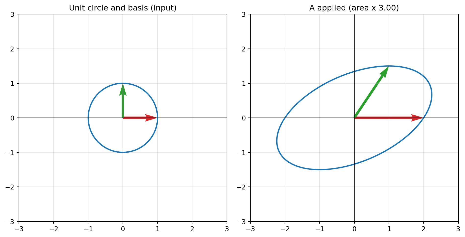
Geometrically, applying \(A\) to the unit circle produces an ellipse whose enclosed area is exactly \(|\det(A)| = 3\) times the original. The code below verifies all of these facts numerically, confirms \(A A^{-1} = I\), checks \(\det(AB) = \det(A)\det(B)\) and \(\text{tr}(AB) = \text{tr}(BA)\), and shows that a deliberately collinear matrix collapses to rank \(1\) with zero determinant.
// Cargo.toml: nalgebra = "0.33"usenalgebra::{Matrix2, Vector2};fn main() {let a =Matrix2::new(2.0,1.0,0.0,1.5);println!("det(A) = {:.4}", a.determinant());println!("tr(A) = {:.4}", a.trace());// Inverse exists because the determinant is nonzeroifletSome(a_inv) = a.try_inverse() {let id = a * a_inv;let err = (id -Matrix2::identity()).abs().max();println!("max|A*Ainv - I| = {:.2e}", err);}// det(AB) = det(A) det(B); tr(AB) = tr(BA)let b =Matrix2::new(1.0,-0.5,0.5,1.0);println!("det(AB)={:.4} det(A)det(B)={:.4}", (a * b).determinant(), a.determinant() * b.determinant());println!("tr(AB)={:.4} tr(BA)={:.4}", (a * b).trace(), (b * a).trace());// Rank-deficient matrix has det 0 and no inverselet a_def =Matrix2::new(1.0,2.0,2.0,4.0);println!("det(singular) = {:.2e} invertible = {}", a_def.determinant(), a_def.try_inverse().is_some());// Solve A x = b without forming the inverselet rhs =Vector2::new(1.0,1.0);ifletSome(x) = a.lu().solve(&rhs) {println!("solution x = {:?}", x);}}
The Python tab runs when the book is built, so its printed output and figure are produced from the actual computation rather than transcribed by hand. The Julia and Rust tabs are idiomatic illustrations of the same checks: Julia’s \ operator and Rust’s lu().solve() both solve \(Ax = b\) by factorization rather than inversion, exactly the practice recommended in Section 4.3.
23.10 References
Axler, S. Linear Algebra Done Right, 4th ed. Undergraduate Texts in Mathematics. Springer, 2024. https://doi.org/10.1007/978-3-031-41026-0
Deisenroth, M. P., Faisal, A. A., and Ong, C. S. Mathematics for Machine Learning. Cambridge University Press, 2020. https://doi.org/10.1017/9781108679930
Hu, E. J., Shen, Y., Wallis, P., Allen-Zhu, Z., Li, Y., Wang, S., Wang, L., and Chen, W. “LoRA: Low-Rank Adaptation of Large Language Models.” International Conference on Learning Representations (ICLR), 2022. https://doi.org/10.48550/arXiv.2106.09685
Vaswani, A., Shazeer, N., Parmar, N., Uszkoreit, J., Jones, L., Gomez, A. N., Kaiser, L., and Polosukhin, I. “Attention Is All You Need.” Advances in Neural Information Processing Systems (NeurIPS), 2017. https://doi.org/10.48550/arXiv.1706.03762
Rezende, D. J., and Mohamed, S. “Variational Inference with Normalizing Flows.” Proceedings of the 32nd International Conference on Machine Learning (ICML), 2015. https://doi.org/10.48550/arXiv.1505.05770
Trefethen, L. N., and Bau, D. Numerical Linear Algebra. Society for Industrial and Applied Mathematics (SIAM), 1997. https://doi.org/10.1137/1.9780898719574
Golub, G. H., and Van Loan, C. F. Matrix Computations, 4th ed. Johns Hopkins University Press, 2013. https://doi.org/10.56021/9781421407944
Harris, C. R., Millman, K. J., van der Walt, S. J., et al. “Array Programming with NumPy.” Nature 585, 357 to 362, 2020. https://doi.org/10.1038/s41586-020-2649-2
Bezanson, J., Edelman, A., Karpinski, S., and Shah, V. B. “Julia: A Fresh Approach to Numerical Computing.” SIAM Review 59(1), 65 to 98, 2017. https://doi.org/10.1137/141000671
Strang, G. Introduction to Linear Algebra, 5th ed. Wellesley-Cambridge Press, 2016. https://doi.org/10.1093/oso/9780980232776.001.0001
Source Code
# Linear Algebra: Matrices and OperationsLinear algebra is the language in which modern machine learning is written. Every forward pass through a neural network, every attention computation in a transformer, and every gradient update during training reduces to a sequence of matrix operations. This chapter develops matrices not as grids of numbers to be manipulated by rote, but as concrete representations of linear maps between vector spaces. We then connect each concept (multiplication, transpose, inverse, rank, determinant, block structure) to how it actually appears inside machine learning systems, where these operations run thousands of times per second across batched tensors on specialized hardware.## 1. Matrices as Linear MapsThe most important idea in this chapter is that a matrix is a function. Specifically, an $m \times n$ matrix $A$ represents a linear map $T : \mathbb{R}^n \to \mathbb{R}^m$ that takes a vector in $n$-dimensional space and produces a vector in $m$-dimensional space.### 1.1 What Linearity MeansA map $T$ is linear when it respects vector addition and scalar multiplication:$$T(\alpha x + \beta y) = \alpha\, T(x) + \beta\, T(y)$$for all vectors $x, y$ and scalars $\alpha, \beta$. This single property has a powerful consequence: a linear map is completely determined by what it does to a basis. If we know where each standard basis vector $e_j = (0, \ldots, 1, \ldots, 0)^\top$ lands, we know where every vector lands, because any vector is a linear combination of basis vectors.Suppose $T(e_j) = a_j$, the $j$-th column of our matrix. Then for $x = \sum_j x_j e_j$,$$T(x) = T\left(\sum_j x_j e_j\right) = \sum_j x_j\, T(e_j) = \sum_j x_j\, a_j.$$This is exactly the matrix-vector product $Ax$. The columns of $A$ are the images of the basis vectors, and $Ax$ forms a linear combination of those columns weighted by the entries of $x$.### 1.2 The Column PictureThis column picture is the single most useful mental model for machine learning practitioners. Reading $Ax$ as a weighted sum of columns explains, for example, why a linear layer with weight matrix $W$ produces outputs that live in the span of $W$'s columns. The output space the model can reach is exactly the column space.```A = [ a_1 | a_2 | ... | a_n ] (columns are images of basis vectors)Ax = x_1 * a_1 + x_2 * a_2 + ... + x_n * a_n```A neural network's expressive power, before nonlinearities are added, is bounded by which directions its weight matrices can produce. Stacking linear maps without nonlinear activations collapses to a single linear map, which is why activation functions are essential: they break the chain of pure linearity that would otherwise make depth pointless.## 2. Matrix Multiplication and Its MeaningIf matrices are linear maps, then matrix multiplication is composition of maps. Given $B : \mathbb{R}^p \to \mathbb{R}^n$ and $A : \mathbb{R}^n \to \mathbb{R}^m$, the composite $A \circ B$ first applies $B$, then $A$, giving a map $\mathbb{R}^p \to \mathbb{R}^m$. The matrix of this composite is the product $AB$.### 2.1 The Definition Follows from CompositionWe do not invent the multiplication rule arbitrarily. We derive it by requiring $(AB)x = A(Bx)$ for every $x$. Write $B$ in terms of its columns and let $x = e_k$, the $k$-th standard basis vector. Then $Bx = B e_k$ is the $k$-th column of $B$, whose $j$-th entry is $B_{jk}$. Applying $A$ gives$$A(B e_k) = A \sum_{j=1}^{n} B_{jk}\, e_j^{(n)} = \sum_{j=1}^{n} B_{jk}\, (A e_j^{(n)}),$$where $A e_j^{(n)}$ is the $j$-th column of $A$, whose $i$-th entry is $A_{ij}$. Reading off the $i$-th entry of the result,$$(AB)_{ik} = \big(A(B e_k)\big)_i = \sum_{j=1}^{n} A_{ij} B_{jk}.$$This formula is forced on us: it is the only rule consistent with composition. The entry in row $i$, column $k$ of the product is the dot product of row $i$ of $A$ with column $k$ of $B$. For this to be defined, the inner dimensions must match: $A$ is $m \times n$ and $B$ is $n \times p$, producing an $m \times p$ result. Associativity $(AB)C = A(BC)$ is then immediate, because composition of functions is associative: both sides send $x$ to the same vector $A(B(Cx))$.### 2.2 Multiple Ways to Read a ProductMatrix multiplication can be read at several levels, and fluency means switching between them freely:1. Entry view: each output entry is a dot product (the formula above).2. Column view: column $k$ of $AB$ equals $A$ applied to column $k$ of $B$. The product transforms each column of $B$.3. Row view: row $i$ of $AB$ equals row $i$ of $A$ times $B$.4. Outer-product view: $AB = \sum_{j} (\text{col}_j A)(\text{row}_j B)$, a sum of rank-one matrices.The outer-product view is especially valuable in machine learning. Low-rank adaptation methods such as LoRA exploit exactly this decomposition, representing a weight update as a sum of a few outer products rather than a full dense matrix, which dramatically reduces the number of trainable parameters.### 2.3 Properties and CostsMatrix multiplication is associative, $(AB)C = A(BC)$, and distributive over addition, but it is not commutative: $AB \neq BA$ in general. Associativity matters for efficiency. Computing $A(BC)$ versus $(AB)C$ can differ enormously in cost depending on the shapes involved, a fact compilers exploit when optimizing computation graphs.The naive cost of multiplying an $m \times n$ by an $n \times p$ matrix is $O(mnp)$ scalar multiply-add operations. Because so much of training time is spent here, hardware accelerators (GPUs and TPUs) are designed around dense matrix multiplication, and a great deal of systems engineering goes into keeping these units busy.## 3. TransposeThe transpose $A^\top$ flips a matrix across its diagonal: $(A^\top)_{ij} = A_{ji}$. An $m \times n$ matrix becomes $n \times m$.### 3.1 The Adjoint InterpretationThe transpose is not merely a bookkeeping operation. It is the adjoint of the linear map with respect to the standard inner product. Concretely, for all vectors $x$ and $y$,$$\langle Ax, y \rangle = \langle x, A^\top y \rangle.$$This is a short computation. With $\langle u, v \rangle = \sum_i u_i v_i$,$$\langle Ax, y \rangle = \sum_i \left(\sum_j A_{ij} x_j\right) y_i = \sum_j x_j \left(\sum_i A_{ij} y_i\right) = \sum_j x_j (A^\top y)_j = \langle x, A^\top y \rangle,$$where the middle step just reorders a finite double sum and recognizes $\sum_i A_{ij} y_i = (A^\top y)_j$. The adjoint property characterizes the transpose uniquely: any matrix $M$ satisfying $\langle Ax, y \rangle = \langle x, My \rangle$ for all $x, y$ must equal $A^\top$.This identity is the engine behind backpropagation. When a linear layer computes $z = Wx$ in the forward pass, the gradient of the loss with respect to the input is obtained by applying $W^\top$ to the upstream gradient:$$\frac{\partial L}{\partial x} = W^\top \frac{\partial L}{\partial z}.$$So the forward pass uses $W$ and the backward pass uses $W^\top$. Every autodiff framework implements this transpose-multiply as the backward rule for a linear layer, which is why the transpose appears constantly in derivations of training algorithms.### 3.2 Useful IdentitiesTwo identities recur often. The transpose of a product reverses the order,$$(AB)^\top = B^\top A^\top.$$We can prove this directly from the entry formula. The $(i,k)$ entry of $(AB)^\top$ is the $(k,i)$ entry of $AB$, namely $\sum_j A_{kj} B_{ji}$. The $(i,k)$ entry of $B^\top A^\top$ is $\sum_j (B^\top)_{ij}(A^\top)_{jk} = \sum_j B_{ji} A_{kj}$, which is the same sum. The adjoint viewpoint gives the same result without indices: $\langle ABx, y\rangle = \langle Bx, A^\top y\rangle = \langle x, B^\top A^\top y\rangle$, so the adjoint of $AB$ is $B^\top A^\top$.A matrix satisfying $A = A^\top$ is called symmetric. Symmetric matrices, particularly those of the form $A^\top A$ (Gram matrices), appear throughout machine learning in covariance estimation, kernel methods, and the normal equations of least squares.## 4. Identity and Inverse### 4.1 The IdentityThe identity matrix $I_n$ is the matrix of the identity map: $I_n x = x$ for every $x$. It has ones on the diagonal and zeros elsewhere, and it acts as the multiplicative neutral element, $AI = A$ and $IA = A$. In residual networks, the skip connection $y = x + F(x)$ can be read as $(I + F)$ applied to the input, and this identity term is what allows gradients to flow cleanly through very deep networks.### 4.2 The InverseA square matrix $A$ is invertible if there exists $A^{-1}$ with$$A A^{-1} = A^{-1} A = I.$$The inverse represents the map that undoes $A$. It exists exactly when $A$ represents a bijection, meaning the linear map loses no information. Equivalently, $A$ is invertible if and only if its columns are linearly independent, its determinant is nonzero, and its rank equals its dimension.The inverse of a product reverses order, mirroring the transpose:$$(AB)^{-1} = B^{-1} A^{-1}.$$The proof is to verify the defining property. Using associativity,$$(AB)(B^{-1} A^{-1}) = A(B B^{-1})A^{-1} = A I A^{-1} = A A^{-1} = I,$$and symmetrically $(B^{-1} A^{-1})(AB) = I$. Since a two-sided inverse is unique (if $CA = I = AD$ then $C = C(AD) = (CA)D = D$), the matrix $B^{-1} A^{-1}$ is exactly $(AB)^{-1}$. A companion identity ties the inverse to the transpose: $(A^\top)^{-1} = (A^{-1})^\top$, because $A^\top (A^{-1})^\top = (A^{-1} A)^\top = I^\top = I$.### 4.3 Why We Rarely Compute InversesIn numerical machine learning, explicitly forming $A^{-1}$ is usually a mistake. Solving the linear system $Ax = b$ directly (for example by LU or Cholesky factorization) is faster and far more numerically stable than computing $A^{-1}$ and then multiplying. The conditioning of $A$ governs how much small perturbations in $b$ get amplified in the solution, and a poorly conditioned matrix can make naive inversion catastrophically inaccurate.```# Prefer this:x = solve(A, b) # factor once, solve# Over this:x = inverse(A) @ b # slower, less stable```This principle carries into second-order optimization. Methods like Newton's method conceptually require the inverse Hessian, but practical implementations solve a linear system or approximate the inverse rather than forming it explicitly.## 5. Rank and NullspaceRank and nullspace describe how much a linear map compresses or preserves information.### 5.1 The Four Fundamental SubspacesEvery $m \times n$ matrix $A$ defines four subspaces. The column space (range) is the set of all outputs $Ax$, living in $\mathbb{R}^m$. The nullspace (kernel) is the set of inputs that map to zero,$$\text{null}(A) = \{ x \in \mathbb{R}^n : Ax = 0 \}.$$The row space and the left nullspace complete the picture, defined symmetrically from $A^\top$. The rank is the dimension of the column space, equivalently the number of linearly independent columns (which always equals the number of linearly independent rows).### 5.2 The Rank-Nullity TheoremThese dimensions are tied together by the rank-nullity theorem:$$\text{rank}(A) + \dim(\text{null}(A)) = n,$$where $n$ is the number of columns. The idea behind the proof is a basis-extension argument. Suppose the nullspace has dimension $k$ with basis $\{u_1, \ldots, u_k\}$. Extend it to a basis of all of $\mathbb{R}^n$ by adding vectors $\{v_1, \ldots, v_{n-k}\}$. One then shows that the images $\{Av_1, \ldots, Av_{n-k}\}$ form a basis of the column space: they span it because the $u_i$ contribute nothing (they map to zero), and they are linearly independent because any dependence among the $Av_j$ would force a combination of the $v_j$ into the nullspace, contradicting that the $v_j$ were chosen outside it. Hence $\text{rank}(A) = n - k$, which rearranges to the theorem. Intuitively, each input dimension either contributes to a distinct output direction (counted in the rank) or gets crushed to zero (counted in the nullspace dimension). The map cannot do both with the same dimension.### 5.3 Rank in Machine LearningRank is central to modern model design. A linear layer with a low-rank weight matrix has limited capacity to mix its inputs, since it can only produce outputs in a low-dimensional column space. This is sometimes a limitation and sometimes a deliberate efficiency choice.Parameter-efficient fine-tuning is the clearest example. LoRA freezes a large pretrained weight matrix $W_0$ and learns a low-rank update $\Delta W = BA$, where $B$ is $d \times r$ and $A$ is $r \times d$ with $r \ll d$. Because the update has rank at most $r$, it requires only $2dr$ parameters instead of $d^2$, yet it captures most of the adaptation needed for a downstream task. The empirical success of LoRA suggests that the useful changes to a pretrained model often live in a low-rank subspace.Rank deficiency also signals redundancy. If a feature matrix has rank below its column count, some features are linear combinations of others, the columns are collinear, and the least-squares solution is not unique. Regularization (ridge, for instance) restores a unique solution by effectively raising the rank of the system being solved.## 6. Trace and DeterminantTwo scalar functions summarize a square matrix in different ways.### 6.1 TraceThe trace is the sum of diagonal entries,$$\text{tr}(A) = \sum_{i} A_{ii}.$$Its most useful property is cyclic invariance: $\text{tr}(ABC) = \text{tr}(BCA) = \text{tr}(CAB)$, and in particular $\text{tr}(AB) = \text{tr}(BA)$ even when $AB$ and $BA$ have different sizes. The base case is a one-line computation. For $A$ of shape $m \times n$ and $B$ of shape $n \times m$,$$\text{tr}(AB) = \sum_{i=1}^{m} (AB)_{ii} = \sum_{i=1}^{m} \sum_{j=1}^{n} A_{ij} B_{ji} = \sum_{j=1}^{n} \sum_{i=1}^{m} B_{ji} A_{ij} = \sum_{j=1}^{n} (BA)_{jj} = \text{tr}(BA),$$where the only move is swapping the order of a finite double sum. The three-factor cyclic identity follows by grouping: $\text{tr}((AB)C) = \text{tr}(C(AB)) = \text{tr}((CA)B) = \text{tr}(B(CA))$. The trace also equals the sum of eigenvalues, which connects it to the total variance captured by a covariance matrix.The trace shows up constantly in machine learning derivations. The squared Frobenius norm of a matrix is $\|A\|_F^2 = \text{tr}(A^\top A)$, and many gradient identities are cleanest when expressed through the trace. The cyclic property is what lets us rearrange terms to extract gradients in matrix calculus.### 6.2 DeterminantThe determinant $\det(A)$ measures how the linear map scales volume. If you apply $A$ to a unit cube, the image is a parallelepiped whose signed volume is $\det(A)$. A determinant of zero means the map flattens space into a lower dimension, which is exactly the condition for non-invertibility. A negative determinant indicates the map reverses orientation.The determinant is multiplicative,$$\det(AB) = \det(A)\det(B),$$which follows from the volume-scaling interpretation: applying $B$ then $A$ scales volume by $\det(B)$ and then by $\det(A)$, so the composite scales by the product. Two consequences are immediate. First, if $A$ is invertible then $\det(A)\det(A^{-1}) = \det(A A^{-1}) = \det(I) = 1$, so $\det(A^{-1}) = 1/\det(A)$, confirming that an invertible matrix has nonzero determinant. Second, the determinant equals the product of eigenvalues, so a zero eigenvalue (a nontrivial nullspace direction) forces $\det(A) = 0$. In machine learning, the determinant appears most prominently in normalizing flows, a class of generative models that transform a simple base distribution through invertible maps. The change-of-variables formula requires the log absolute determinant of the Jacobian,$$\log p_X(x) = \log p_Z(f(x)) + \log\left| \det \frac{\partial f}{\partial x} \right|,$$so flow architectures are deliberately designed (with triangular or coupling structures) to make this determinant cheap to compute. It also appears in the log-likelihood of a multivariate Gaussian, where the term $\log\det(\Sigma)$ penalizes overly spread-out covariance estimates.## 7. Block MatricesLarge matrices in practice are rarely treated as undifferentiated grids. They are organized into blocks, submatrices that can themselves be manipulated as units.### 7.1 Block OperationsA block matrix partitions rows and columns into groups. When the partitions are compatible, multiplication works at the block level exactly as it does at the scalar level:$$\begin{bmatrix} A & B \\ C & D \end{bmatrix} \begin{bmatrix} E & F \\ G & H \end{bmatrix} = \begin{bmatrix} AE + BG & AF + BH \\ CE + DG & CF + DH \end{bmatrix}.$$This is more than notation. Treating blocks as units is how high-performance libraries tile matrix multiplication to fit cache and memory hierarchies, processing one block at a time so that data stays in fast memory while it is reused.### 7.2 Block Structure in ModelsBlock thinking pervades model architecture. A transformer computes queries, keys, and values by projecting the input through three weight matrices that are often concatenated into a single block matrix $W_{qkv} = [W_q \mid W_k \mid W_v]$ and applied in one fused operation, then split. Multi-head attention partitions the embedding dimension into blocks, one per head, each attending independently before the results are concatenated.Block-diagonal matrices, where off-diagonal blocks are zero, represent maps that act independently on separate groups of coordinates. Grouped convolutions and mixture-of-experts routing both have this flavor: different parts of the input are processed by different parameter blocks, which saves computation and can be parallelized across devices.## 8. Batched Operations in Machine LearningEverything above describes single matrices acting on single vectors. Real machine learning systems operate on batches, and understanding the batch dimension is essential to reading model code and reasoning about performance.### 8.1 The Linear LayerA linear (fully connected) layer applies an affine map $y = Wx + b$. With weight matrix $W$ of shape $m \times n$, it sends an $n$-dimensional input to an $m$-dimensional output. But we almost never feed one example at a time. Instead we stack $B$ examples into a matrix $X$ of shape $B \times n$, one example per row, and compute$$Y = X W^\top + b,$$where $Y$ has shape $B \times m$ and the bias $b$ is broadcast across rows. The transpose appears because of the row-major convention: with examples as rows, applying the map to every row at once is a single matrix multiplication. This one operation processes the entire batch, and it maps directly onto the matrix-multiply units of a GPU, which is why batching is the foundation of efficient training and inference.### 8.2 Batched Matrix MultiplicationBeyond stacking vectors, modern architectures multiply stacks of matrices. A batched matrix multiply (often called bmm) takes two tensors of shape $B \times n \times p$ and $B \times p \times q$ and produces $B \times n \times q$, performing $B$ independent matrix products in parallel:$$Z_b = X_b\, Y_b, \qquad b = 1, \ldots, B.$$The leading dimension (sometimes several leading dimensions) is treated as a batch over which the same operation runs independently. Attention is the canonical consumer. For each example and each head, the scores are computed as$$\text{scores} = \frac{Q K^\top}{\sqrt{d_k}},$$where $Q$ and $K$ are matrices of shape (sequence length) by (head dimension), and this product is batched over both the example index and the head index. The softmax-weighted combination with the value matrix $V$ is another batched product. A single attention layer therefore issues a large collection of small matrix multiplications, all dispatched together.### 8.3 Broadcasting and Shape DisciplineBatched code relies on broadcasting, the rule by which arrays of different but compatible shapes are aligned by implicitly repeating along size-one dimensions. Adding a bias vector of shape $m$ to an output of shape $B \times m$ works because the bias is broadcast across the batch. Getting these shapes right is a large part of practical machine learning engineering, and shape mismatches are among the most common bugs.```# Conceptual shapes in an attention layerQ, K, V : (B, heads, seq, d_head)scores = Q @ K.transpose(-2, -1) # (B, heads, seq, seq)attn = softmax(scores / sqrt(d_head))out = attn @ V # (B, heads, seq, d_head)```### 8.4 Why This Framing MattersSeeing these operations as batched linear algebra, rather than as opaque library calls, pays off in several ways. It clarifies where the computation actually goes, since the bulk of training time lives in a handful of large matrix multiplications. It explains memory cost, since intermediate tensors like the attention score matrix scale with the square of the sequence length. And it guides optimization, because techniques such as operator fusion, mixed precision, and low-rank factorization all amount to restructuring these same matrix operations to do less work or use the hardware more fully. The practitioner who reads a model as a graph of batched linear maps can reason about its cost and behavior with confidence.## 9. A Worked Numerical ExampleTo make the abstractions concrete, take the $2 \times 2$ matrix$$A = \begin{bmatrix} 2 & 1 \\ 0 & \tfrac{3}{2} \end{bmatrix}.$$We can read off every quantity from this chapter by hand. The trace is $\text{tr}(A) = 2 + \tfrac{3}{2} = \tfrac{7}{2}$. Because $A$ is upper triangular, its determinant is the product of the diagonal entries, $\det(A) = 2 \cdot \tfrac{3}{2} = 3$, and the eigenvalues are exactly those diagonal entries, $\lambda_1 = 2$ and $\lambda_2 = \tfrac{3}{2}$. As a sanity check, the eigenvalues sum to $\tfrac{7}{2}$ (the trace) and multiply to $3$ (the determinant), matching the general identities.Since $\det(A) = 3 \neq 0$, the map is invertible and full rank ($\text{rank}(A) = 2$, so by rank-nullity the nullspace is $\{0\}$). The inverse of an upper-triangular $2 \times 2$ matrix is$$A^{-1} = \frac{1}{\det(A)} \begin{bmatrix} \tfrac{3}{2} & -1 \\ 0 & 2 \end{bmatrix} = \begin{bmatrix} \tfrac{1}{2} & -\tfrac{1}{3} \\ 0 & \tfrac{2}{3} \end{bmatrix}.$$Geometrically, applying $A$ to the unit circle produces an ellipse whose enclosed area is exactly $|\det(A)| = 3$ times the original. The code below verifies all of these facts numerically, confirms $A A^{-1} = I$, checks $\det(AB) = \det(A)\det(B)$ and $\text{tr}(AB) = \text{tr}(BA)$, and shows that a deliberately collinear matrix collapses to rank $1$ with zero determinant.::: {.panel-tabset}## Python```{python}import numpy as npimport matplotlib.pyplot as pltrng = np.random.default_rng(19)A = np.array([[2.0, 1.0], [0.0, 1.5]])# Numerical checks of the chapter's claimsrank = np.linalg.matrix_rank(A)det = np.linalg.det(A)tr = np.trace(A)eigvals = np.linalg.eigvals(A)print(f"rank(A) = {rank}")print(f"det(A) = {det:.4f} (prod eigenvalues = {np.prod(eigvals).real:.4f})")print(f"tr(A) = {tr:.4f} (sum eigenvalues = {np.sum(eigvals).real:.4f})")# Inverse exists because det != 0; verify A @ A_inv = IA_inv = np.linalg.inv(A)print(f"max|A A^-1 - I| = {np.max(np.abs(A @ A_inv - np.eye(2))):.2e}")# det(AB) = det(A) det(B) and tr(AB) = tr(BA)B = np.array([[1.0, -0.5], [0.5, 1.0]])print(f"det(AB)={np.linalg.det(A @ B):.4f} "f"det(A)det(B)={np.linalg.det(A) * np.linalg.det(B):.4f}")print(f"tr(AB)={np.trace(A @ B):.4f} tr(BA)={np.trace(B @ A):.4f}")# Rank-deficient matrix: column 2 = 2 * column 1A_def = np.array([[1.0, 2.0], [2.0, 4.0]])print(f"rank(singular)={np.linalg.matrix_rank(A_def)} "f"det={np.linalg.det(A_def):.2e}")# Visualize the map acting on the unit circle and the basis vectorstheta = np.linspace(0, 2* np.pi, 200)circle = np.vstack([np.cos(theta), np.sin(theta)])mapped = A @ circlee1 = np.array([1.0, 0.0])e2 = np.array([0.0, 1.0])Ae1 = A @ e1Ae2 = A @ e2fig, ax = plt.subplots(1, 2, figsize=(10, 5))ax[0].plot(circle[0], circle[1], lw=2, color="tab:blue")ax[0].quiver(0, 0, e1[0], e1[1], angles="xy", scale_units="xy", scale=1, color="tab:red", width=0.012)ax[0].quiver(0, 0, e2[0], e2[1], angles="xy", scale_units="xy", scale=1, color="tab:green", width=0.012)ax[0].set_title("Unit circle and basis (input)")ax[1].plot(mapped[0], mapped[1], lw=2, color="tab:blue")ax[1].quiver(0, 0, Ae1[0], Ae1[1], angles="xy", scale_units="xy", scale=1, color="tab:red", width=0.012)ax[1].quiver(0, 0, Ae2[0], Ae2[1], angles="xy", scale_units="xy", scale=1, color="tab:green", width=0.012)ax[1].set_title(f"A applied (area x {det:.2f})")for a in ax: a.set_aspect("equal") a.grid(True, alpha=0.3) a.set_xlim(-3, 3) a.set_ylim(-3, 3) a.axhline(0, color="black", lw=0.6) a.axvline(0, color="black", lw=0.6)fig.tight_layout()plt.show()```## Julia```juliausingLinearAlgebraA = [2.01.0;0.01.5]println("rank(A) = ", rank(A))println("det(A) = ", det(A), " (prod eig = ", prod(eigvals(A)), ")")println("tr(A) = ", tr(A), " (sum eig = ", sum(eigvals(A)), ")")# Inverse and identity checkAinv =inv(A)println("max|A*Ainv - I| = ", maximum(abs.(A * Ainv - I)))# Multiplicative determinant and cyclic traceB = [1.0-0.5; 0.51.0]println("det(AB) = ", det(A * B), " det(A)det(B) = ", det(A) *det(B))println("tr(AB) = ", tr(A * B), " tr(BA) = ", tr(B * A))# Rank-deficient matrixAdef = [1.02.0; 2.04.0]println("rank(singular) = ", rank(Adef), " det = ", det(Adef))# Solve a system rather than forming the inverseb = [1.0, 1.0]x = A \ bprintln("solution x = ", x)```## Rust```rust// Cargo.toml: nalgebra ="0.33"use nalgebra::{Matrix2, Vector2};fn main() { let a = Matrix2::new(2.0, 1.0,0.0, 1.5); println!("det(A) = {:.4}", a.determinant()); println!("tr(A) = {:.4}", a.trace());// Inverse exists because the determinant is nonzeroif let Some(a_inv) =a.try_inverse() { let id = a * a_inv; let err = (id - Matrix2::identity()).abs().max(); println!("max|A*Ainv - I| = {:.2e}", err); }//det(AB) =det(A) det(B); tr(AB) =tr(BA) let b = Matrix2::new(1.0, -0.5,0.5, 1.0); println!("det(AB)={:.4} det(A)det(B)={:.4}", (a * b).determinant(), a.determinant() *b.determinant()); println!("tr(AB)={:.4} tr(BA)={:.4}", (a * b).trace(), (b * a).trace());// Rank-deficient matrix has det 0 and no inverse let a_def = Matrix2::new(1.0, 2.0,2.0, 4.0); println!("det(singular) = {:.2e} invertible = {}",a_def.determinant(), a_def.try_inverse().is_some());// Solve A x = b without forming the inverse let rhs = Vector2::new(1.0, 1.0);if let Some(x) =a.lu().solve(&rhs) { println!("solution x = {:?}", x); }}```:::The Python tab runs when the book is built, so its printed output and figure are produced from the actual computation rather than transcribed by hand. The Julia and Rust tabs are idiomatic illustrations of the same checks: Julia's `\` operator and Rust's `lu().solve()` both solve $Ax = b$ by factorization rather than inversion, exactly the practice recommended in Section 4.3.## References1. Axler, S. *Linear Algebra Done Right*, 4th ed. Undergraduate Texts in Mathematics. Springer, 2024. https://doi.org/10.1007/978-3-031-41026-02. Deisenroth, M. P., Faisal, A. A., and Ong, C. S. *Mathematics for Machine Learning*. Cambridge University Press, 2020. https://doi.org/10.1017/97811086799303. Hu, E. J., Shen, Y., Wallis, P., Allen-Zhu, Z., Li, Y., Wang, S., Wang, L., and Chen, W. "LoRA: Low-Rank Adaptation of Large Language Models." International Conference on Learning Representations (ICLR), 2022. https://doi.org/10.48550/arXiv.2106.096854. Vaswani, A., Shazeer, N., Parmar, N., Uszkoreit, J., Jones, L., Gomez, A. N., Kaiser, L., and Polosukhin, I. "Attention Is All You Need." Advances in Neural Information Processing Systems (NeurIPS), 2017. https://doi.org/10.48550/arXiv.1706.037625. Rezende, D. J., and Mohamed, S. "Variational Inference with Normalizing Flows." Proceedings of the 32nd International Conference on Machine Learning (ICML), 2015. https://doi.org/10.48550/arXiv.1505.057706. Trefethen, L. N., and Bau, D. *Numerical Linear Algebra*. Society for Industrial and Applied Mathematics (SIAM), 1997. https://doi.org/10.1137/1.97808987195747. Golub, G. H., and Van Loan, C. F. *Matrix Computations*, 4th ed. Johns Hopkins University Press, 2013. https://doi.org/10.56021/97814214079448. Harris, C. R., Millman, K. J., van der Walt, S. J., et al. "Array Programming with NumPy." *Nature* 585, 357 to 362, 2020. https://doi.org/10.1038/s41586-020-2649-29. Bezanson, J., Edelman, A., Karpinski, S., and Shah, V. B. "Julia: A Fresh Approach to Numerical Computing." *SIAM Review* 59(1), 65 to 98, 2017. https://doi.org/10.1137/14100067110. Strang, G. *Introduction to Linear Algebra*, 5th ed. Wellesley-Cambridge Press, 2016. https://doi.org/10.1093/oso/9780980232776.001.0001