Modern statistical learning routinely confronts problems where the number of candidate predictors rivals or exceeds the number of observations. In genomics a single experiment may measure tens of thousands of gene expression levels for a few hundred patients. In natural language processing a bag-of-words representation produces a feature for every token in a vocabulary. In these high-dimensional regimes ordinary least squares either fails outright, because the design matrix is rank deficient, or it overfits catastrophically, fitting noise as though it were signal. The Lasso, introduced by Tibshirani in 1996, addresses both problems at once by adding an \(\ell_1\) penalty to the least squares objective. The penalty shrinks coefficients toward zero and, crucially, sets many of them exactly to zero. The result is a model that performs estimation and variable selection simultaneously, yielding sparse and interpretable solutions. This chapter develops the geometry, optimization, and probabilistic interpretation of the Lasso, then turns to its use as a feature selection engine.
90.1 1. The L1 Penalty and the Lasso Estimator
90.1.1 1.1 From Ridge to Lasso
Consider a linear model \(y = X\beta + \varepsilon\) with response vector \(y \in \mathbb{R}^n\), design matrix \(X \in \mathbb{R}^{n \times p}\), and coefficient vector \(\beta \in \mathbb{R}^p\). Ordinary least squares minimizes the residual sum of squares \(\|y - X\beta\|_2^2\). When \(p\) is large relative to \(n\), regularization is needed to control variance. Ridge regression adds a squared \(\ell_2\) penalty, while the Lasso adds an \(\ell_1\) penalty:
where \(\|\beta\|_1 = \sum_{j=1}^p |\beta_j|\) and \(\lambda \geq 0\) is a tuning parameter that governs the strength of regularization. Both penalties shrink coefficients, but only the \(\ell_1\) penalty produces exact zeros. This single change in the choice of norm has profound consequences for the structure of the solution.
It is conventional to standardize the columns of \(X\) to have zero mean and unit variance before fitting, and to center \(y\), so that the intercept can be handled separately and the penalty treats all coefficients on a comparable scale. We assume this standardization throughout.
90.1.2 1.2 The Constrained Formulation
By Lagrangian duality the penalized problem is equivalent to a constrained one. For every \(\lambda\) there exists a budget \(t\) such that
As \(\lambda\) increases from zero to infinity, the corresponding budget \(t\) decreases from the unconstrained least squares norm down to zero. This constrained view is the key to understanding why the Lasso produces sparsity, because the geometry of the constraint region determines where the optimal solution lands.
90.2 2. Why L1 Induces Sparsity: The Geometry
90.2.1 2.1 Constraint Sets and Contours
The least squares objective \(\|y - X\beta\|_2^2\) has elliptical contours centered at the unconstrained minimizer \(\hat{\beta}^{\text{ols}}\). The optimization seeks the point inside the constraint region that lies on the lowest reachable contour, which is the point where an expanding ellipse first touches the constraint set.
For ridge regression the constraint \(\|\beta\|_2 \leq t\) is a ball, which is perfectly round in every dimension. The point of tangency between an ellipse and a ball almost never has any coordinate exactly equal to zero. For the Lasso the constraint \(\|\beta\|_1 \leq t\) is a cross-polytope: in two dimensions a diamond with vertices on the axes, in higher dimensions an object with sharp corners and edges aligned with coordinate subspaces. The \(\ell_1\) ball in \(\mathbb{R}^p\) has \(2p\) vertices, each of the form \(\pm t\, e_j\) where \(e_j\) is a standard basis vector, and these vertices are exactly the maximally sparse points of the ball, with a single nonzero coordinate. Lower-dimensional faces of the polytope are spanned by subsets of the axes, so every face of dimension \(d\) forces \(p - d\) coefficients to vanish. Because the ellipse is most likely to first touch this region at a corner or low-dimensional edge, and those features lie on the axes where one or more coordinates vanish, the Lasso solution tends to be sparse. The key contrast is local geometry: at a vertex the boundary of the \(\ell_1\) ball has a nonsmooth kink supporting a whole cone of outward normals, so a positive-measure set of objective gradients is balanced there, whereas the smooth \(\ell_2\) sphere admits exactly one outward normal at each point and so pins the solution to a sparse axis only on a measure-zero set of gradient directions. The non-differentiable kinks of the \(\ell_1\) ball are precisely what create exact zeros.
90.2.2 2.2 The Subgradient Condition
We can make this precise with the optimality conditions. The Lasso objective is convex but not differentiable at points where some \(\beta_j = 0\). The relevant tool is the subgradient. At a minimizer the zero vector must belong to the subdifferential of the objective. Writing the stationarity condition coordinate by coordinate gives, for each \(j\),
where \(x_j\) is the \(j\)-th column of \(X\) and \(s_j\) is a component of a subgradient of \(\|\beta\|_1\). To see where this comes from, recall the definition of the subdifferential of a convex function \(f\) at a point \(\beta\): it is the set of all vectors \(g\) such that \(f(\beta') \geq f(\beta) + g^\top(\beta' - \beta)\) for every \(\beta'\). For the absolute value \(|\cdot|\) the subdifferential is the singleton \(\{\operatorname{sign}(\beta_j)\}\) away from the origin and the whole interval \([-1, 1]\) at the origin, because at the kink any slope between \(-1\) and \(+1\) supports the function from below. A point \(\hat{\beta}\) minimizes the convex objective if and only if \(0\) lies in the subdifferential, which gives the coordinatewise stationarity condition above. The condition for a coefficient to be zero is therefore
In words, a feature is dropped from the model whenever its correlation with the current residual is smaller in magnitude than the threshold \(\lambda\). Features that fail to clear this bar contribute nothing. This is a hard, discrete decision embedded inside a continuous convex problem, and it is the algebraic source of sparsity. Contrast this with the ridge condition, \(-x_j^\top(y - X\hat{\beta}) + \lambda \hat{\beta}_j = 0\), which can only be satisfied with \(\hat{\beta}_j = 0\) when the residual correlation is exactly zero, an event of measure zero.
90.2.3 2.3 The Orthonormal Case and Soft Thresholding
When the columns of \(X\) are orthonormal, so that \(X^\top X = I\), the Lasso decouples across coordinates and admits a closed-form solution. Expanding the objective and using orthonormality, \(\|y - X\beta\|_2^2 = \|y\|_2^2 - 2\beta^\top X^\top y + \beta^\top \beta\), which is separable across coordinates up to the constant \(\|y\|_2^2\). Let \(z_j = x_j^\top y\) be the OLS coefficient. Each coordinate then minimizes the scalar function
For \(\beta_j > 0\) the derivative is \(2\beta_j - 2z_j + \lambda\), which vanishes at \(\beta_j = z_j - \lambda/2\), valid only when \(z_j > \lambda/2\). For \(\beta_j < 0\) the derivative is \(2\beta_j - 2z_j - \lambda\), vanishing at \(\beta_j = z_j + \lambda/2\), valid only when \(z_j < -\lambda/2\). When \(|z_j| \leq \lambda/2\) neither branch is active and the subgradient condition \(0 \in [-2z_j - \lambda, -2z_j + \lambda]\) holds at \(\beta_j = 0\). Collecting the three cases gives
where \((\cdot)_+\) denotes the positive part and \(S\) is the soft thresholding operator. This formula captures the dual nature of the Lasso. Coefficients whose magnitude is below the threshold are set exactly to zero, which is selection, and surviving coefficients are pulled toward zero by a constant amount, which is shrinkage. Ridge regression in the same setting gives \(\hat{\beta}_j = z_j / (1 + \lambda)\), a proportional shrinkage that never reaches zero. Soft thresholding is the atom from which coordinate descent algorithms are built.
90.3 3. Computing the Lasso
90.3.1 3.1 Coordinate Descent
The dominant algorithm for fitting the Lasso at scale is cyclic coordinate descent. The idea is to optimize one coordinate at a time, holding the others fixed, and to cycle through the coordinates until convergence. Because the penalty \(\|\beta\|_1\) is separable across coordinates and the loss is smooth, each one-dimensional subproblem has the soft thresholding solution from the orthonormal case.
Fixing all coefficients except \(\beta_j\), define the partial residual \(r^{(j)} = y - \sum_{k \neq j} x_k \hat{\beta}_k\). The one-dimensional subproblem is to minimize, over the scalar \(\beta_j\),
where the loss has been scaled by \(\tfrac{1}{2}\) to keep the algebra clean. Expanding the quadratic, \(\tfrac{1}{2}\|r^{(j)}\|_2^2 - \beta_j\, x_j^\top r^{(j)} + \tfrac{1}{2}\beta_j^2 \|x_j\|_2^2\). For the standardized design with \(\|x_j\|_2^2 = 1\) this is precisely the orthonormal scalar problem solved above with \(z_j = x_j^\top r^{(j)}\) and penalty \(\lambda\), so the minimizer is the soft thresholded inner product
When the loss is written without the \(\tfrac{1}{2}\) factor, as in the orthonormal display earlier, the threshold is \(\lambda/2\); the two conventions differ only by how \(\lambda\) is scaled. Each update is an inner product and a thresholding, both cheap. The procedure converges to the global optimum because the objective is convex and the nonsmooth part separates. The algorithm becomes especially efficient when warm starts and active set strategies are combined: one fits the model along a decreasing grid of \(\lambda\) values, using the solution at one \(\lambda\) to initialize the next, and restricts updates to the set of coordinates likely to be nonzero. This is the strategy implemented in the widely used glmnet package.
# Cyclic coordinate descent for the Lasso (schematic)
initialize beta = 0
repeat until convergence:
    for j in 1..p:
        r_j = y - X[:, -j] @ beta[-j]      # partial residual
        rho = X[:, j].T @ r_j               # correlation with residual
        beta[j] = sign(rho) * max(abs(rho) - lambda/2, 0)
90.3.2 3.2 Least Angle Regression and the Solution Path
A different and historically important algorithm is Least Angle Regression (LARS), due to Efron, Hastie, Johnstone, and Tibshirani. LARS computes the entire Lasso path, meaning the full trajectory of \(\hat{\beta}(\lambda)\) as \(\lambda\) varies, rather than a solution at a single \(\lambda\). The key structural fact is that the Lasso path is piecewise linear in \(\lambda\): between successive breakpoints, called knots, each active coefficient changes linearly. LARS exploits this by jumping directly from knot to knot.
The algorithm begins with all coefficients zero and identifies the predictor most correlated with the response. It then moves the coefficient of that predictor in the direction of its correlation, but only until a second predictor becomes equally correlated with the residual. At that point both predictors are added to the active set and the coefficients move together along the equiangular direction that keeps all active predictors tied in correlation. The process continues, adding predictors as they catch up. A small modification, which removes a variable from the active set if its coefficient hits zero, makes LARS compute the exact Lasso path. Because the entire path is produced in roughly the cost of a single least squares fit, LARS is attractive when one wants to inspect the order in which variables enter the model.
90.3.3 3.3 Choosing the Tuning Parameter
The penalty \(\lambda\) controls the bias-variance trade-off. Large \(\lambda\) yields a sparse, high-bias, low-variance model; small \(\lambda\) approaches OLS. The standard practical choice is \(k\)-fold cross-validation: fit the Lasso path on each training fold, evaluate prediction error on the held-out fold across the \(\lambda\) grid, and average. Two rules are common. The minimum-error rule selects the \(\lambda\) minimizing the average cross-validated error. The one-standard-error rule selects the largest \(\lambda\) whose error is within one standard error of the minimum, favoring a more parsimonious model with comparable predictive accuracy.
90.4 4. The Laplace Prior View
90.4.1 4.1 Penalized Likelihood as Maximum a Posteriori Estimation
Regularized estimators have a clean Bayesian reading. Suppose the data follow a Gaussian linear model, \(y \mid \beta \sim \mathcal{N}(X\beta, \sigma^2 I)\), so that the negative log likelihood is proportional to \(\|y - X\beta\|_2^2 / (2\sigma^2)\). Place an independent prior on each coefficient and the maximum a posteriori (MAP) estimate maximizes the log posterior, which equals the log likelihood plus the log prior. Different priors yield different penalties. A Gaussian prior \(\beta_j \sim \mathcal{N}(0, \tau^2)\) contributes a squared penalty and recovers ridge regression.
For the Lasso the relevant prior is the Laplace, or double exponential, distribution:
Its log density is \(-|\beta_j|/b\) up to a constant, so the sum over coordinates contributes a term proportional to \(\|\beta\|_1\). To make the correspondence explicit, the negative log posterior is
Multiplying through by \(2\sigma^2\) leaves the minimizer unchanged and recovers the penalized least squares objective \(\|y - X\beta\|_2^2 + \lambda \|\beta\|_1\) with the correspondence \(\lambda = 2\sigma^2 / b\). The MAP estimate under independent Laplace priors is therefore exactly the Lasso. A smaller scale \(b\) concentrates the prior more tightly at the origin and translates into a larger \(\lambda\) and stronger shrinkage. The sharp peak of the Laplace density at the origin, much sharper than the Gaussian, expresses a prior belief that many coefficients are at or near zero, which is the probabilistic counterpart of sparsity.
90.4.2 4.2 What the Prior View Buys and What It Hides
The Laplace interpretation is illuminating but carries a caveat. The Lasso is the posterior mode, not the posterior mean. Under a Laplace prior the posterior distribution generally assigns zero probability to the event that any coefficient is exactly zero, so the posterior mean is dense even though the mode is sparse. The exact zeros of the Lasso are an artifact of mode-finding against a non-differentiable prior, not a property of the full posterior. This observation motivated genuinely sparse Bayesian alternatives, such as spike-and-slab priors that place positive probability mass exactly at zero, and continuous shrinkage priors like the horseshoe that mimic sparsity through heavy tails and an infinite spike at the origin. These deliver uncertainty quantification that the point-estimate Lasso does not.
90.5 5. Feature Selection with the Lasso
90.5.1 5.1 The Lasso as a Selector
Because the Lasso sets coefficients exactly to zero, the set of nonzero coefficients \(\hat{S} = \{ j : \hat{\beta}_j \neq 0 \}\) is a selected subset of features. This embedded selection is the Lasso’s signature advantage over ridge in interpretation-driven applications. Unlike wrapper methods that search over an exponential number of subsets, the Lasso identifies a model in convex, polynomial time. The number of selected features is controlled smoothly by \(\lambda\), and in the standard formulation the Lasso selects at most \(\min(n, p)\) variables, a consequence of the geometry of the problem.
90.5.2 5.2 Conditions for Correct Recovery
A natural theoretical question is whether the selected set \(\hat{S}\) recovers the true support \(S\) of the data-generating coefficients. The answer depends on how correlated the relevant predictors are with the irrelevant ones. The central sufficient condition is the irrepresentable condition, which requires that the irrelevant predictors cannot be too well represented by the relevant ones:
When this holds, and with an appropriately chosen \(\lambda\) and adequate signal strength, the Lasso recovers the correct support with high probability. When it fails, typically because of strong correlation among features, the Lasso may include spurious variables or miss true ones. A related and milder condition, the restricted eigenvalue condition, suffices for the weaker guarantee of accurate estimation in \(\ell_2\) error even when exact support recovery is out of reach.
90.5.3 5.3 Bias, the Adaptive Lasso, and Debiasing
The same shrinkage that enables selection also biases the surviving coefficients toward zero, since soft thresholding subtracts a constant from each nonzero estimate. This bias can degrade both prediction and the accuracy of selection. Several remedies exist. The relaxed Lasso refits an unpenalized least squares model on the selected support \(\hat{S}\), removing the shrinkage bias from the retained coefficients. The adaptive Lasso applies coordinate-specific weights \(w_j\) to the penalty,
with weights such as \(w_j = 1 / |\hat{\beta}_j^{\text{init}}|^\gamma\) derived from an initial estimate. Large initial coefficients receive small weights and are penalized lightly, while small ones are penalized heavily, which yields the oracle property: under suitable conditions the adaptive Lasso selects the correct support and estimates the nonzero coefficients as well as if the support had been known in advance.
90.5.4 5.4 Correlated Features and the Elastic Net
A practical weakness of the Lasso is its behavior under groups of highly correlated predictors. When several features are nearly collinear, the Lasso tends to select one arbitrarily and zero out the rest, which is unstable and can be misleading when the goal is to identify all relevant variables. The elastic net addresses this by combining the \(\ell_1\) and \(\ell_2\) penalties:
The \(\ell_2\) term introduces a grouping effect, encouraging correlated predictors to enter or leave the model together and stabilizing selection, while the \(\ell_1\) term preserves sparsity. The elastic net also lifts the \(\min(n, p)\) ceiling on the number of selected variables, which matters when the true model is denser than \(n\) in the \(p \gg n\) regime. In practice the elastic net is often the default choice for high-dimensional problems with correlated features, with the mixing between the two penalties tuned alongside the overall strength.
90.5.5 5.5 A Practical Workflow
A standard applied pipeline ties these pieces together. Standardize the features, fit a Lasso or elastic net path over a grid of penalty values using coordinate descent with warm starts, choose the penalty by cross-validation under the one-standard-error rule for parsimony, and optionally refit an unpenalized model on the selected support to debias the coefficients. When inference on the selected coefficients is required, naive p-values computed after selection are invalid because the same data chose the model and tested it, and one should turn to post-selection inference methods or stability selection, which assesses how often each feature is chosen across resampled subsets.
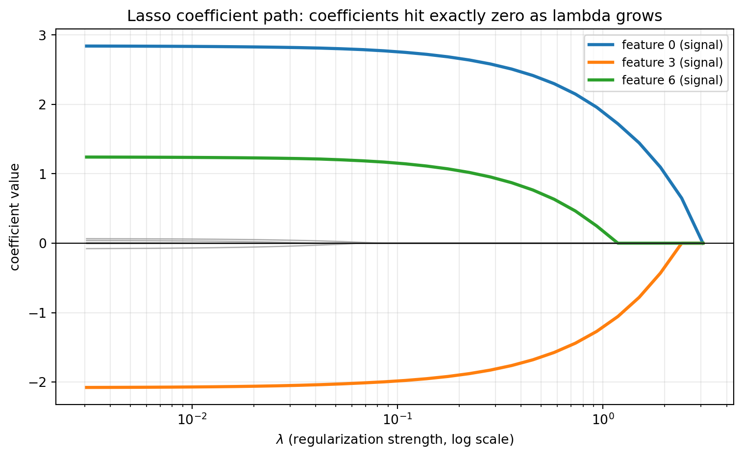
The example below computes a full Lasso path on a synthetic problem where only three of ten features are truly relevant. As the penalty grows, irrelevant coefficients are driven to exactly zero, leaving the true support, before excessive shrinkage starts biasing the survivors.
import numpy as npimport matplotlib.pyplot as pltfrom sklearn.linear_model import lasso_pathfrom sklearn.preprocessing import StandardScalerrng = np.random.default_rng(0)# Synthetic regression: only 3 of 10 features are truly relevant.n, p =120, 10X = rng.standard_normal((n, p))true_beta = np.zeros(p)true_beta[[0, 3, 6]] = [3.0, -2.0, 1.5]y = X @ true_beta +0.5* rng.standard_normal(n)# Standardize features and center the response.X = StandardScaler().fit_transform(X)y = y - y.mean()# Compute the Lasso path over a grid of penalties.alphas, coefs, _ = lasso_path(X, y, n_alphas=30)print("Truly nonzero features:", np.flatnonzero(true_beta).tolist())print(f"{'lambda':>10}{'n_nonzero':>10} selected")for k inrange(0, len(alphas), 6): beta = coefs[:, k] sel = np.flatnonzero(np.abs(beta) >1e-8).tolist()print(f"{alphas[k]:10.4f}{len(sel):10d}{sel}")# Visualize the coefficient path versus the penalty lambda. As lambda grows# the L1 penalty drives coefficients to exactly zero, so the irrelevant# features collapse onto the zero line while the three true signals persist.relevant =set(np.flatnonzero(true_beta).tolist())fig, ax = plt.subplots(figsize=(8, 5))for j inrange(p):if j in relevant: ax.plot(alphas, coefs[j], lw=2.4, label=f"feature {j} (signal)")else: ax.plot(alphas, coefs[j], lw=1.0, color="0.6", alpha=0.8)ax.set_xscale("log")ax.axhline(0.0, color="black", lw=0.8)ax.set_xlabel(r"$\lambda$(regularization strength, log scale)")ax.set_ylabel("coefficient value")ax.set_title("Lasso coefficient path: coefficients hit exactly zero as lambda grows")ax.legend(loc="upper right", fontsize=9)ax.grid(True, which="both", alpha=0.25)fig.tight_layout()plt.show()
The Lasso replaces the squared penalty of ridge regression with an \(\ell_1\) penalty, a small change with large consequences. Geometrically the cross-polytope constraint has corners on the coordinate axes, so the least squares ellipse tends to touch it where coefficients vanish. Algebraically the subgradient optimality condition thresholds each feature against its residual correlation, producing exact zeros through soft thresholding. The estimator is computed efficiently by coordinate descent, while LARS traces the entire piecewise-linear solution path. Probabilistically the Lasso is the MAP estimate under a sparsity-favoring Laplace prior, a view that clarifies its behavior while reminding us that the exact zeros live in the mode rather than the full posterior. As a feature selector the Lasso performs estimation and selection jointly in polynomial time, with recovery guaranteed under conditions on feature correlation, and its known limitations under collinearity and shrinkage bias are addressed by the adaptive Lasso, the relaxed Lasso, and the elastic net. Together these tools make \(\ell_1\) regularization one of the most useful instruments in the modern high-dimensional toolkit.
90.7 References
Tibshirani, R. (1996). Regression Shrinkage and Selection via the Lasso. Journal of the Royal Statistical Society, Series B, 58(1), 267 to 288. https://doi.org/10.1111/j.2517-6161.1996.tb02080.x
Efron, B., Hastie, T., Johnstone, I., and Tibshirani, R. (2004). Least Angle Regression. Annals of Statistics, 32(2), 407 to 499. https://doi.org/10.1214/009053604000000067
Friedman, J., Hastie, T., and Tibshirani, R. (2010). Regularization Paths for Generalized Linear Models via Coordinate Descent. Journal of Statistical Software, 33(1), 1 to 22. https://doi.org/10.18637/jss.v033.i01
Zou, H., and Hastie, T. (2005). Regularization and Variable Selection via the Elastic Net. Journal of the Royal Statistical Society, Series B, 67(2), 301 to 320. https://doi.org/10.1111/j.1467-9868.2005.00503.x
Zou, H. (2006). The Adaptive Lasso and Its Oracle Properties. Journal of the American Statistical Association, 101(476), 1418 to 1429. https://doi.org/10.1198/016214506000000735
Zhao, P., and Yu, B. (2006). On Model Selection Consistency of Lasso. Journal of Machine Learning Research, 7, 2541 to 2563. https://www.jmlr.org/papers/v7/zhao06a.html
Park, T., and Casella, G. (2008). The Bayesian Lasso. Journal of the American Statistical Association, 103(482), 681 to 686. https://doi.org/10.1198/016214508000000337
Hastie, T., Tibshirani, R., and Friedman, J. (2009). The Elements of Statistical Learning, 2nd ed. Springer. https://doi.org/10.1007/978-0-387-84858-7
Hastie, T., Tibshirani, R., and Wainwright, M. (2015). Statistical Learning with Sparsity: The Lasso and Generalizations. CRC Press. https://doi.org/10.1201/b18401
Source Code
# Lasso and Sparsity: L1 RegularizationModern statistical learning routinely confronts problems where the number of candidate predictors rivals or exceeds the number of observations. In genomics a single experiment may measure tens of thousands of gene expression levels for a few hundred patients. In natural language processing a bag-of-words representation produces a feature for every token in a vocabulary. In these high-dimensional regimes ordinary least squares either fails outright, because the design matrix is rank deficient, or it overfits catastrophically, fitting noise as though it were signal. The Lasso, introduced by Tibshirani in 1996, addresses both problems at once by adding an $\ell_1$ penalty to the least squares objective. The penalty shrinks coefficients toward zero and, crucially, sets many of them exactly to zero. The result is a model that performs estimation and variable selection simultaneously, yielding sparse and interpretable solutions. This chapter develops the geometry, optimization, and probabilistic interpretation of the Lasso, then turns to its use as a feature selection engine.## 1. The L1 Penalty and the Lasso Estimator### 1.1 From Ridge to LassoConsider a linear model $y = X\beta + \varepsilon$ with response vector $y \in \mathbb{R}^n$, design matrix $X \in \mathbb{R}^{n \times p}$, and coefficient vector $\beta \in \mathbb{R}^p$. Ordinary least squares minimizes the residual sum of squares $\|y - X\beta\|_2^2$. When $p$ is large relative to $n$, regularization is needed to control variance. Ridge regression adds a squared $\ell_2$ penalty, while the Lasso adds an $\ell_1$ penalty:$$\hat{\beta}^{\text{ridge}} = \arg\min_{\beta} \; \|y - X\beta\|_2^2 + \lambda \|\beta\|_2^2, \qquad\hat{\beta}^{\text{lasso}} = \arg\min_{\beta} \; \|y - X\beta\|_2^2 + \lambda \|\beta\|_1,$$where $\|\beta\|_1 = \sum_{j=1}^p |\beta_j|$ and $\lambda \geq 0$ is a tuning parameter that governs the strength of regularization. Both penalties shrink coefficients, but only the $\ell_1$ penalty produces exact zeros. This single change in the choice of norm has profound consequences for the structure of the solution.It is conventional to standardize the columns of $X$ to have zero mean and unit variance before fitting, and to center $y$, so that the intercept can be handled separately and the penalty treats all coefficients on a comparable scale. We assume this standardization throughout.### 1.2 The Constrained FormulationBy Lagrangian duality the penalized problem is equivalent to a constrained one. For every $\lambda$ there exists a budget $t$ such that$$\hat{\beta}^{\text{lasso}} = \arg\min_{\beta} \; \|y - X\beta\|_2^2 \quad \text{subject to} \quad \|\beta\|_1 \leq t.$$As $\lambda$ increases from zero to infinity, the corresponding budget $t$ decreases from the unconstrained least squares norm down to zero. This constrained view is the key to understanding why the Lasso produces sparsity, because the geometry of the constraint region determines where the optimal solution lands.## 2. Why L1 Induces Sparsity: The Geometry### 2.1 Constraint Sets and ContoursThe least squares objective $\|y - X\beta\|_2^2$ has elliptical contours centered at the unconstrained minimizer $\hat{\beta}^{\text{ols}}$. The optimization seeks the point inside the constraint region that lies on the lowest reachable contour, which is the point where an expanding ellipse first touches the constraint set.For ridge regression the constraint $\|\beta\|_2 \leq t$ is a ball, which is perfectly round in every dimension. The point of tangency between an ellipse and a ball almost never has any coordinate exactly equal to zero. For the Lasso the constraint $\|\beta\|_1 \leq t$ is a cross-polytope: in two dimensions a diamond with vertices on the axes, in higher dimensions an object with sharp corners and edges aligned with coordinate subspaces. The $\ell_1$ ball in $\mathbb{R}^p$ has $2p$ vertices, each of the form $\pm t\, e_j$ where $e_j$ is a standard basis vector, and these vertices are exactly the maximally sparse points of the ball, with a single nonzero coordinate. Lower-dimensional faces of the polytope are spanned by subsets of the axes, so every face of dimension $d$ forces $p - d$ coefficients to vanish. Because the ellipse is most likely to first touch this region at a corner or low-dimensional edge, and those features lie on the axes where one or more coordinates vanish, the Lasso solution tends to be sparse. The key contrast is local geometry: at a vertex the boundary of the $\ell_1$ ball has a nonsmooth kink supporting a whole cone of outward normals, so a positive-measure set of objective gradients is balanced there, whereas the smooth $\ell_2$ sphere admits exactly one outward normal at each point and so pins the solution to a sparse axis only on a measure-zero set of gradient directions. The non-differentiable kinks of the $\ell_1$ ball are precisely what create exact zeros.### 2.2 The Subgradient ConditionWe can make this precise with the optimality conditions. The Lasso objective is convex but not differentiable at points where some $\beta_j = 0$. The relevant tool is the subgradient. At a minimizer the zero vector must belong to the subdifferential of the objective. Writing the stationarity condition coordinate by coordinate gives, for each $j$,$$-x_j^\top (y - X\hat{\beta}) + \lambda \, s_j = 0, \qquads_j \in\begin{cases}\{\operatorname{sign}(\hat{\beta}_j)\} & \hat{\beta}_j \neq 0, \\[-1, 1] & \hat{\beta}_j = 0,\end{cases}$$where $x_j$ is the $j$-th column of $X$ and $s_j$ is a component of a subgradient of $\|\beta\|_1$. To see where this comes from, recall the definition of the subdifferential of a convex function $f$ at a point $\beta$: it is the set of all vectors $g$ such that $f(\beta') \geq f(\beta) + g^\top(\beta' - \beta)$ for every $\beta'$. For the absolute value $|\cdot|$ the subdifferential is the singleton $\{\operatorname{sign}(\beta_j)\}$ away from the origin and the whole interval $[-1, 1]$ at the origin, because at the kink any slope between $-1$ and $+1$ supports the function from below. A point $\hat{\beta}$ minimizes the convex objective if and only if $0$ lies in the subdifferential, which gives the coordinatewise stationarity condition above. The condition for a coefficient to be zero is therefore$$\left| x_j^\top (y - X\hat{\beta}) \right| \leq \lambda.$$In words, a feature is dropped from the model whenever its correlation with the current residual is smaller in magnitude than the threshold $\lambda$. Features that fail to clear this bar contribute nothing. This is a hard, discrete decision embedded inside a continuous convex problem, and it is the algebraic source of sparsity. Contrast this with the ridge condition, $-x_j^\top(y - X\hat{\beta}) + \lambda \hat{\beta}_j = 0$, which can only be satisfied with $\hat{\beta}_j = 0$ when the residual correlation is exactly zero, an event of measure zero.### 2.3 The Orthonormal Case and Soft ThresholdingWhen the columns of $X$ are orthonormal, so that $X^\top X = I$, the Lasso decouples across coordinates and admits a closed-form solution. Expanding the objective and using orthonormality, $\|y - X\beta\|_2^2 = \|y\|_2^2 - 2\beta^\top X^\top y + \beta^\top \beta$, which is separable across coordinates up to the constant $\|y\|_2^2$. Let $z_j = x_j^\top y$ be the OLS coefficient. Each coordinate then minimizes the scalar function$$f(\beta_j) = \beta_j^2 - 2 z_j \beta_j + \lambda |\beta_j|.$$For $\beta_j > 0$ the derivative is $2\beta_j - 2z_j + \lambda$, which vanishes at $\beta_j = z_j - \lambda/2$, valid only when $z_j > \lambda/2$. For $\beta_j < 0$ the derivative is $2\beta_j - 2z_j - \lambda$, vanishing at $\beta_j = z_j + \lambda/2$, valid only when $z_j < -\lambda/2$. When $|z_j| \leq \lambda/2$ neither branch is active and the subgradient condition $0 \in [-2z_j - \lambda, -2z_j + \lambda]$ holds at $\beta_j = 0$. Collecting the three cases gives$$\hat{\beta}_j^{\text{lasso}} = \operatorname{sign}(z_j)\,\bigl(|z_j| - \lambda/2\bigr)_+ = S_{\lambda/2}(z_j),$$where $(\cdot)_+$ denotes the positive part and $S$ is the soft thresholding operator. This formula captures the dual nature of the Lasso. Coefficients whose magnitude is below the threshold are set exactly to zero, which is selection, and surviving coefficients are pulled toward zero by a constant amount, which is shrinkage. Ridge regression in the same setting gives $\hat{\beta}_j = z_j / (1 + \lambda)$, a proportional shrinkage that never reaches zero. Soft thresholding is the atom from which coordinate descent algorithms are built.## 3. Computing the Lasso### 3.1 Coordinate DescentThe dominant algorithm for fitting the Lasso at scale is cyclic coordinate descent. The idea is to optimize one coordinate at a time, holding the others fixed, and to cycle through the coordinates until convergence. Because the penalty $\|\beta\|_1$ is separable across coordinates and the loss is smooth, each one-dimensional subproblem has the soft thresholding solution from the orthonormal case.Fixing all coefficients except $\beta_j$, define the partial residual $r^{(j)} = y - \sum_{k \neq j} x_k \hat{\beta}_k$. The one-dimensional subproblem is to minimize, over the scalar $\beta_j$,$$g(\beta_j) = \tfrac{1}{2}\,\bigl\| r^{(j)} - x_j \beta_j \bigr\|_2^2 + \lambda |\beta_j|,$$where the loss has been scaled by $\tfrac{1}{2}$ to keep the algebra clean. Expanding the quadratic, $\tfrac{1}{2}\|r^{(j)}\|_2^2 - \beta_j\, x_j^\top r^{(j)} + \tfrac{1}{2}\beta_j^2 \|x_j\|_2^2$. For the standardized design with $\|x_j\|_2^2 = 1$ this is precisely the orthonormal scalar problem solved above with $z_j = x_j^\top r^{(j)}$ and penalty $\lambda$, so the minimizer is the soft thresholded inner product$$\hat{\beta}_j \leftarrow S_{\lambda}\!\left( x_j^\top r^{(j)} \right)= \operatorname{sign}\!\left( x_j^\top r^{(j)} \right) \bigl( |x_j^\top r^{(j)}| - \lambda \bigr)_+ .$$When the loss is written without the $\tfrac{1}{2}$ factor, as in the orthonormal display earlier, the threshold is $\lambda/2$; the two conventions differ only by how $\lambda$ is scaled. Each update is an inner product and a thresholding, both cheap. The procedure converges to the global optimum because the objective is convex and the nonsmooth part separates. The algorithm becomes especially efficient when warm starts and active set strategies are combined: one fits the model along a decreasing grid of $\lambda$ values, using the solution at one $\lambda$ to initialize the next, and restricts updates to the set of coordinates likely to be nonzero. This is the strategy implemented in the widely used `glmnet` package.```text# Cyclic coordinate descent for the Lasso (schematic)initialize beta = 0repeat until convergence: for j in 1..p: r_j = y - X[:, -j] @ beta[-j] # partial residual rho = X[:, j].T @ r_j # correlation with residual beta[j] = sign(rho) * max(abs(rho) - lambda/2, 0)```### 3.2 Least Angle Regression and the Solution PathA different and historically important algorithm is Least Angle Regression (LARS), due to Efron, Hastie, Johnstone, and Tibshirani. LARS computes the entire Lasso path, meaning the full trajectory of $\hat{\beta}(\lambda)$ as $\lambda$ varies, rather than a solution at a single $\lambda$. The key structural fact is that the Lasso path is piecewise linear in $\lambda$: between successive breakpoints, called knots, each active coefficient changes linearly. LARS exploits this by jumping directly from knot to knot.The algorithm begins with all coefficients zero and identifies the predictor most correlated with the response. It then moves the coefficient of that predictor in the direction of its correlation, but only until a second predictor becomes equally correlated with the residual. At that point both predictors are added to the active set and the coefficients move together along the equiangular direction that keeps all active predictors tied in correlation. The process continues, adding predictors as they catch up. A small modification, which removes a variable from the active set if its coefficient hits zero, makes LARS compute the exact Lasso path. Because the entire path is produced in roughly the cost of a single least squares fit, LARS is attractive when one wants to inspect the order in which variables enter the model.### 3.3 Choosing the Tuning ParameterThe penalty $\lambda$ controls the bias-variance trade-off. Large $\lambda$ yields a sparse, high-bias, low-variance model; small $\lambda$ approaches OLS. The standard practical choice is $k$-fold cross-validation: fit the Lasso path on each training fold, evaluate prediction error on the held-out fold across the $\lambda$ grid, and average. Two rules are common. The minimum-error rule selects the $\lambda$ minimizing the average cross-validated error. The one-standard-error rule selects the largest $\lambda$ whose error is within one standard error of the minimum, favoring a more parsimonious model with comparable predictive accuracy.## 4. The Laplace Prior View### 4.1 Penalized Likelihood as Maximum a Posteriori EstimationRegularized estimators have a clean Bayesian reading. Suppose the data follow a Gaussian linear model, $y \mid \beta \sim \mathcal{N}(X\beta, \sigma^2 I)$, so that the negative log likelihood is proportional to $\|y - X\beta\|_2^2 / (2\sigma^2)$. Place an independent prior on each coefficient and the maximum a posteriori (MAP) estimate maximizes the log posterior, which equals the log likelihood plus the log prior. Different priors yield different penalties. A Gaussian prior $\beta_j \sim \mathcal{N}(0, \tau^2)$ contributes a squared penalty and recovers ridge regression.For the Lasso the relevant prior is the Laplace, or double exponential, distribution:$$p(\beta_j) = \frac{1}{2b} \exp\!\left( -\frac{|\beta_j|}{b} \right).$$Its log density is $-|\beta_j|/b$ up to a constant, so the sum over coordinates contributes a term proportional to $\|\beta\|_1$. To make the correspondence explicit, the negative log posterior is$$-\log p(\beta \mid y) = \frac{1}{2\sigma^2}\|y - X\beta\|_2^2 + \frac{1}{b}\sum_{j=1}^p |\beta_j| + \text{const}.$$Multiplying through by $2\sigma^2$ leaves the minimizer unchanged and recovers the penalized least squares objective $\|y - X\beta\|_2^2 + \lambda \|\beta\|_1$ with the correspondence $\lambda = 2\sigma^2 / b$. The MAP estimate under independent Laplace priors is therefore exactly the Lasso. A smaller scale $b$ concentrates the prior more tightly at the origin and translates into a larger $\lambda$ and stronger shrinkage. The sharp peak of the Laplace density at the origin, much sharper than the Gaussian, expresses a prior belief that many coefficients are at or near zero, which is the probabilistic counterpart of sparsity.### 4.2 What the Prior View Buys and What It HidesThe Laplace interpretation is illuminating but carries a caveat. The Lasso is the posterior mode, not the posterior mean. Under a Laplace prior the posterior distribution generally assigns zero probability to the event that any coefficient is exactly zero, so the posterior mean is dense even though the mode is sparse. The exact zeros of the Lasso are an artifact of mode-finding against a non-differentiable prior, not a property of the full posterior. This observation motivated genuinely sparse Bayesian alternatives, such as spike-and-slab priors that place positive probability mass exactly at zero, and continuous shrinkage priors like the horseshoe that mimic sparsity through heavy tails and an infinite spike at the origin. These deliver uncertainty quantification that the point-estimate Lasso does not.## 5. Feature Selection with the Lasso### 5.1 The Lasso as a SelectorBecause the Lasso sets coefficients exactly to zero, the set of nonzero coefficients $\hat{S} = \{ j : \hat{\beta}_j \neq 0 \}$ is a selected subset of features. This embedded selection is the Lasso's signature advantage over ridge in interpretation-driven applications. Unlike wrapper methods that search over an exponential number of subsets, the Lasso identifies a model in convex, polynomial time. The number of selected features is controlled smoothly by $\lambda$, and in the standard formulation the Lasso selects at most $\min(n, p)$ variables, a consequence of the geometry of the problem.### 5.2 Conditions for Correct RecoveryA natural theoretical question is whether the selected set $\hat{S}$ recovers the true support $S$ of the data-generating coefficients. The answer depends on how correlated the relevant predictors are with the irrelevant ones. The central sufficient condition is the irrepresentable condition, which requires that the irrelevant predictors cannot be too well represented by the relevant ones:$$\left\| X_{S^c}^\top X_S \left( X_S^\top X_S \right)^{-1} \operatorname{sign}(\beta_S) \right\|_\infty < 1.$$When this holds, and with an appropriately chosen $\lambda$ and adequate signal strength, the Lasso recovers the correct support with high probability. When it fails, typically because of strong correlation among features, the Lasso may include spurious variables or miss true ones. A related and milder condition, the restricted eigenvalue condition, suffices for the weaker guarantee of accurate estimation in $\ell_2$ error even when exact support recovery is out of reach.### 5.3 Bias, the Adaptive Lasso, and DebiasingThe same shrinkage that enables selection also biases the surviving coefficients toward zero, since soft thresholding subtracts a constant from each nonzero estimate. This bias can degrade both prediction and the accuracy of selection. Several remedies exist. The relaxed Lasso refits an unpenalized least squares model on the selected support $\hat{S}$, removing the shrinkage bias from the retained coefficients. The adaptive Lasso applies coordinate-specific weights $w_j$ to the penalty,$$\hat{\beta} = \arg\min_{\beta} \; \|y - X\beta\|_2^2 + \lambda \sum_{j=1}^p w_j |\beta_j|,$$with weights such as $w_j = 1 / |\hat{\beta}_j^{\text{init}}|^\gamma$ derived from an initial estimate. Large initial coefficients receive small weights and are penalized lightly, while small ones are penalized heavily, which yields the oracle property: under suitable conditions the adaptive Lasso selects the correct support and estimates the nonzero coefficients as well as if the support had been known in advance.### 5.4 Correlated Features and the Elastic NetA practical weakness of the Lasso is its behavior under groups of highly correlated predictors. When several features are nearly collinear, the Lasso tends to select one arbitrarily and zero out the rest, which is unstable and can be misleading when the goal is to identify all relevant variables. The elastic net addresses this by combining the $\ell_1$ and $\ell_2$ penalties:$$\hat{\beta} = \arg\min_{\beta} \; \|y - X\beta\|_2^2 + \lambda_1 \|\beta\|_1 + \lambda_2 \|\beta\|_2^2.$$The $\ell_2$ term introduces a grouping effect, encouraging correlated predictors to enter or leave the model together and stabilizing selection, while the $\ell_1$ term preserves sparsity. The elastic net also lifts the $\min(n, p)$ ceiling on the number of selected variables, which matters when the true model is denser than $n$ in the $p \gg n$ regime. In practice the elastic net is often the default choice for high-dimensional problems with correlated features, with the mixing between the two penalties tuned alongside the overall strength.### 5.5 A Practical WorkflowA standard applied pipeline ties these pieces together. Standardize the features, fit a Lasso or elastic net path over a grid of penalty values using coordinate descent with warm starts, choose the penalty by cross-validation under the one-standard-error rule for parsimony, and optionally refit an unpenalized model on the selected support to debias the coefficients. When inference on the selected coefficients is required, naive p-values computed after selection are invalid because the same data chose the model and tested it, and one should turn to post-selection inference methods or stability selection, which assesses how often each feature is chosen across resampled subsets.The example below computes a full Lasso path on a synthetic problem where only three of ten features are truly relevant. As the penalty grows, irrelevant coefficients are driven to exactly zero, leaving the true support, before excessive shrinkage starts biasing the survivors.::: {.panel-tabset}## Python```{python}import numpy as npimport matplotlib.pyplot as pltfrom sklearn.linear_model import lasso_pathfrom sklearn.preprocessing import StandardScalerrng = np.random.default_rng(0)# Synthetic regression: only 3 of 10 features are truly relevant.n, p =120, 10X = rng.standard_normal((n, p))true_beta = np.zeros(p)true_beta[[0, 3, 6]] = [3.0, -2.0, 1.5]y = X @ true_beta +0.5* rng.standard_normal(n)# Standardize features and center the response.X = StandardScaler().fit_transform(X)y = y - y.mean()# Compute the Lasso path over a grid of penalties.alphas, coefs, _ = lasso_path(X, y, n_alphas=30)print("Truly nonzero features:", np.flatnonzero(true_beta).tolist())print(f"{'lambda':>10}{'n_nonzero':>10} selected")for k inrange(0, len(alphas), 6): beta = coefs[:, k] sel = np.flatnonzero(np.abs(beta) >1e-8).tolist()print(f"{alphas[k]:10.4f}{len(sel):10d}{sel}")# Visualize the coefficient path versus the penalty lambda. As lambda grows# the L1 penalty drives coefficients to exactly zero, so the irrelevant# features collapse onto the zero line while the three true signals persist.relevant =set(np.flatnonzero(true_beta).tolist())fig, ax = plt.subplots(figsize=(8, 5))for j inrange(p):if j in relevant: ax.plot(alphas, coefs[j], lw=2.4, label=f"feature {j} (signal)")else: ax.plot(alphas, coefs[j], lw=1.0, color="0.6", alpha=0.8)ax.set_xscale("log")ax.axhline(0.0, color="black", lw=0.8)ax.set_xlabel(r"$\lambda$(regularization strength, log scale)")ax.set_ylabel("coefficient value")ax.set_title("Lasso coefficient path: coefficients hit exactly zero as lambda grows")ax.legend(loc="upper right", fontsize=9)ax.grid(True, which="both", alpha=0.25)fig.tight_layout()plt.show()```## Julia```julia# Illustrative: Lasso path with GLMNet.jlusingGLMNet, Random, StatisticsRandom.seed!(0)n, p =120, 10X =randn(n, p)beta =zeros(p); beta[[1, 4, 7]] = [3.0, -2.0, 1.5]y = X * beta .+0.5.*randn(n)# Standardize columns; GLMNet fits the full path internally.X = (X .-mean(X, dims=1)) ./std(X, dims=1)path =glmnet(X, y .-mean(y)) # alpha defaults to 1.0 (Lasso)for k in1:6:length(path.lambda) sel =findall(!iszero, path.betas[:, k])println("lambda=", round(path.lambda[k], digits=4), " selected=", sel)end```## Rust```rust// Illustrative: one cyclic coordinate-descent sweep with soft thresholding.fn soft_threshold(z: f64, lam: f64) -> f64 {z.signum() * (z.abs() - lam).max(0.0)}fn lasso_cd(x:&[Vec<f64>], y:&[f64], lam: f64, iters: usize) -> Vec<f64> {let (n, p) = (x.len(), x[0].len()); let mut beta = vec![0.0; p];for _ in0..iters {for j in0..p {// Partial residual correlation, assuming standardized columns. let mut rho =0.0;for i in0..n { let pred: f64 = (0..p).filter(|&k| k != j).map(|k| x[i][k] * beta[k]).sum(); rho += x[i][j] * (y[i] - pred); } beta[j] =soft_threshold(rho / n as f64, lam); } } beta}```:::## 6. SummaryThe Lasso replaces the squared penalty of ridge regression with an $\ell_1$ penalty, a small change with large consequences. Geometrically the cross-polytope constraint has corners on the coordinate axes, so the least squares ellipse tends to touch it where coefficients vanish. Algebraically the subgradient optimality condition thresholds each feature against its residual correlation, producing exact zeros through soft thresholding. The estimator is computed efficiently by coordinate descent, while LARS traces the entire piecewise-linear solution path. Probabilistically the Lasso is the MAP estimate under a sparsity-favoring Laplace prior, a view that clarifies its behavior while reminding us that the exact zeros live in the mode rather than the full posterior. As a feature selector the Lasso performs estimation and selection jointly in polynomial time, with recovery guaranteed under conditions on feature correlation, and its known limitations under collinearity and shrinkage bias are addressed by the adaptive Lasso, the relaxed Lasso, and the elastic net. Together these tools make $\ell_1$ regularization one of the most useful instruments in the modern high-dimensional toolkit.## References1. Tibshirani, R. (1996). Regression Shrinkage and Selection via the Lasso. Journal of the Royal Statistical Society, Series B, 58(1), 267 to 288. https://doi.org/10.1111/j.2517-6161.1996.tb02080.x2. Efron, B., Hastie, T., Johnstone, I., and Tibshirani, R. (2004). Least Angle Regression. Annals of Statistics, 32(2), 407 to 499. https://doi.org/10.1214/0090536040000000673. Friedman, J., Hastie, T., and Tibshirani, R. (2010). Regularization Paths for Generalized Linear Models via Coordinate Descent. Journal of Statistical Software, 33(1), 1 to 22. https://doi.org/10.18637/jss.v033.i014. Zou, H., and Hastie, T. (2005). Regularization and Variable Selection via the Elastic Net. Journal of the Royal Statistical Society, Series B, 67(2), 301 to 320. https://doi.org/10.1111/j.1467-9868.2005.00503.x5. Zou, H. (2006). The Adaptive Lasso and Its Oracle Properties. Journal of the American Statistical Association, 101(476), 1418 to 1429. https://doi.org/10.1198/0162145060000007356. Zhao, P., and Yu, B. (2006). On Model Selection Consistency of Lasso. Journal of Machine Learning Research, 7, 2541 to 2563. https://www.jmlr.org/papers/v7/zhao06a.html7. Park, T., and Casella, G. (2008). The Bayesian Lasso. Journal of the American Statistical Association, 103(482), 681 to 686. https://doi.org/10.1198/0162145080000003378. Hastie, T., Tibshirani, R., and Friedman, J. (2009). The Elements of Statistical Learning, 2nd ed. Springer. https://doi.org/10.1007/978-0-387-84858-79. Hastie, T., Tibshirani, R., and Wainwright, M. (2015). Statistical Learning with Sparsity: The Lasso and Generalizations. CRC Press. https://doi.org/10.1201/b18401