Gradient descent is the workhorse optimization procedure behind nearly every modern neural network. Before practitioners reach for adaptive methods such as Adam or momentum-based schemes, it pays to understand the plain, first-order algorithm in its purest form. This chapter develops vanilla gradient descent rigorously: the update rule, the three sampling regimes (batch, stochastic, and mini-batch), the role of the learning rate, the geometry of the loss surface, and the convergence behavior that ties these elements together.
196.1 1. The Optimization Problem
A neural network defines a parametric function \(f_\theta : \mathcal{X} \to \mathcal{Y}\), where \(\theta \in \mathbb{R}^d\) collects all weights and biases. Given a dataset \(\{(x_i, y_i)\}_{i=1}^{n}\) and a per-example loss \(\ell(\cdot, \cdot)\), training seeks parameters that minimize the empirical risk
This is the objective that gradient descent attacks. The function \(L : \mathbb{R}^d \to \mathbb{R}\) is generally non-convex in \(\theta\) because of the nested nonlinearities in \(f_\theta\), so we cannot expect a closed-form minimizer. Instead we iterate.
The defining idea is local. At any point \(\theta\), the negative gradient \(-\nabla L(\theta)\) is the direction of steepest descent of \(L\). To first order,
so a small step \(\delta = -\eta\, \nabla L(\theta)\) with \(\eta > 0\) decreases the objective whenever the gradient is nonzero. The scalar \(\eta\) is the learning rate, and the recursion
is the vanilla gradient descent update. Everything else in this chapter is a refinement of, or a perspective on, this single equation.
196.2 2. Computing the Gradient
For neural networks the gradient \(\nabla L(\theta)\) is obtained by backpropagation, which is reverse-mode automatic differentiation applied to the computational graph of \(f_\theta\). Because the loss is an average over examples, linearity of differentiation gives
This decomposition is the seam along which the batch, stochastic, and mini-batch variants split. Each variant estimates the full-data gradient from a different number of summands.
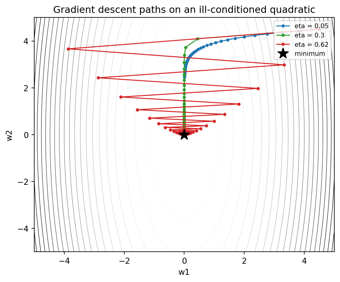
A minimal description of one full-batch step looks like the following. The cell below runs vanilla gradient descent on an ill-conditioned 2D quadratic for three learning rates and plots the trajectories on a contour map of the loss surface. The blue path crawls (eta too small), green descends cleanly, and red zig-zags as it nears the stability limit 2 / lambda_max.
Code
import numpy as npimport matplotlib.pyplot as pltnp.random.seed(0)# Anisotropic quadratic L(w) = 0.5 * w^T H w, eigenvalues 3.0 and 0.3H = np.array([[3.0, 0.0], [0.0, 0.3]])def grad(w):return H @ wdef loss(w):return0.5* w @ H @ wdef descend(w0, eta, steps=40): w = np.array(w0, dtype=float) path = [w.copy()]for _ inrange(steps): w = w - eta * grad(w) path.append(w.copy())return np.array(path)w0 = np.array([4.5, 4.5])etas = [0.05, 0.30, 0.62] # 2 / lambda_max = 0.667 is the stability limitcolors = ["tab:blue", "tab:green", "tab:red"]gx = np.linspace(-5, 5, 200)GX, GY = np.meshgrid(gx, gx)Z =0.5* (H[0, 0] * GX**2+ H[1, 1] * GY**2)fig, ax = plt.subplots(figsize=(6, 5))ax.contour(GX, GY, Z, levels=20, cmap="Greys", linewidths=0.6)for eta, c inzip(etas, colors): p = descend(w0, eta) ax.plot(p[:, 0], p[:, 1], "o-", ms=3, lw=1.2, color=c, label=f"eta = {eta}")print(f"eta={eta}: final loss={loss(p[-1]):.4e}")ax.plot(0, 0, "k*", ms=14, label="minimum")ax.set_xlabel("w1"); ax.set_ylabel("w2")ax.set_title("Gradient descent paths on an ill-conditioned quadratic")ax.legend(loc="upper right", fontsize=8)plt.tight_layout()plt.show()
eta=0.05: final loss=9.0667e-01
eta=0.3: final loss=1.6063e-03
eta=0.62: final loss=1.7496e-04
196.3 3. Batch, Stochastic, and Mini-Batch Descent
196.3.1 3.1 Batch Gradient Descent
Batch (or full-batch) gradient descent uses the exact gradient computed over all \(n\) examples at every step. The update is precisely the recursion of Section 1. Its appeal is determinism: given \(\theta_t\), the next iterate \(\theta_{t+1}\) is fixed, and the trajectory descends the true loss surface monotonically when \(\eta\) is small enough. Its drawback is cost. Each step requires a forward and backward pass over the entire dataset, which is prohibitive when \(n\) reaches millions of examples. For large datasets the method also wastes computation, since the gradient direction stabilizes long before all examples are processed.
196.3.2 3.2 Stochastic Gradient Descent
Stochastic gradient descent (SGD) goes to the opposite extreme. At each step it draws a single index \(i_t\) uniformly at random and updates using only that example:
This unbiasedness is what makes SGD work: on average it steps in the correct direction. The cost per step is constant in \(n\), so SGD makes rapid progress in the early phase of training. The price is variance. Individual updates are noisy, and the iterates jitter around the descent path rather than following it smoothly. As we discuss in Section 6, this noise is not purely harmful, because it can help the iterates escape sharp, poorly generalizing regions of the loss surface.
196.3.3 3.3 Mini-Batch Gradient Descent
Mini-batch gradient descent is the practical compromise that dominates deep learning. At each step it samples a subset \(B_t \subset \{1, \dots, n\}\) of size \(m\) (the batch size) and uses the average gradient over the mini-batch:
Like the single-example gradient, \(g_t\) is unbiased for \(\nabla L(\theta_t)\). Its variance, however, scales as \(1/m\) for independent samples, so larger batches yield smoother, more reliable steps. Mini-batches also map well onto hardware: matrix multiplications over a batch of \(m\) examples saturate the parallelism of GPUs and TPUs in a way that single examples cannot. Typical values of \(m\) range from 32 to a few thousand, chosen to balance gradient quality, memory, and throughput.
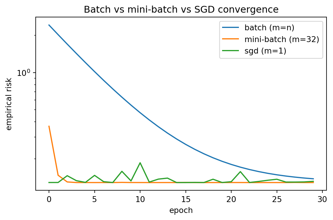
The cell below realizes all three regimes on a linear-regression empirical risk, varying only the batch size m. Batch descent (m = n) gives the smoothest curve, SGD (m = 1) the noisiest, and the mini-batch (m = 32) interpolates, all driving the risk down per epoch.
Code
import numpy as npimport matplotlib.pyplot as pltrng = np.random.default_rng(42)n, d =400, 1X = rng.normal(size=(n, d))true_w = np.array([2.5])y = X @ true_w +0.5* rng.normal(size=n)def full_loss(w): r = X @ w - yreturn0.5* np.mean(r**2)def grad_on(idx, w): r = X[idx] @ w - y[idx]return X[idx].T @ r /len(idx)def train(batch_size, eta, epochs=30): w = np.zeros(d) hist = []for _ inrange(epochs): order = rng.permutation(n)for start inrange(0, n, batch_size): idx = order[start:start + batch_size] w = w - eta * grad_on(idx, w) hist.append(full_loss(w))return np.array(hist)regimes = {"batch (m=n)": n, "mini-batch (m=32)": 32, "sgd (m=1)": 1}fig, ax = plt.subplots(figsize=(6, 4))for name, m in regimes.items(): hist = train(m, eta=0.1) ax.plot(hist, label=name)print(f"{name}: final empirical risk={hist[-1]:.4e}")ax.set_xlabel("epoch"); ax.set_ylabel("empirical risk")ax.set_yscale("log")ax.set_title("Batch vs mini-batch vs SGD convergence")ax.legend()plt.tight_layout()plt.show()
batch (m=n): final empirical risk=1.3819e-01
mini-batch (m=32): final empirical risk=1.2881e-01
sgd (m=1): final empirical risk=1.3176e-01
A useful unifying view: all three methods share the update \(\theta_{t+1} = \theta_t - \eta\, g_t\), and they differ only in how \(g_t\) is formed. Batch descent sets \(m = n\) and has zero estimation variance; SGD sets \(m = 1\) and has maximal variance; mini-batch interpolates. One pass through the data, however the batches are drawn, is called an epoch.
196.4 4. The Learning Rate
The learning rate \(\eta\) is the single most consequential hyperparameter in gradient descent. It controls the size of each step, and its effect is best understood through a local quadratic model. Suppose near a minimum \(L\) is well approximated by
where \(H = \nabla^2 L(\theta^\star)\) is the Hessian, assumed positive definite with eigenvalues \(0 < \lambda_{\min} \le \cdots \le \lambda_{\max}\). Gradient descent on this quadratic decouples along the eigenvectors of \(H\). Along the eigenvector with eigenvalue \(\lambda\), the error contracts by the factor \(|1 - \eta \lambda|\) each step. Three regimes follow.
If \(\eta < 2 / \lambda_{\max}\), every mode contracts and the iterates converge.
If \(\eta = 1 / \lambda\), the corresponding mode is solved in a single step.
If \(\eta > 2 / \lambda_{\max}\), the steepest mode diverges and the loss blows up.
The convergence rate is governed by the worst-contracting mode, and the optimal learning rate that minimizes \(\max_\lambda |1 - \eta \lambda|\) is
which yields a contraction factor of \((\kappa - 1)/(\kappa + 1)\) where \(\kappa = \lambda_{\max} / \lambda_{\min}\) is the condition number. When \(\kappa\) is large, the surface is ill conditioned: a learning rate small enough to keep the steep direction stable is far too small for the flat direction, so progress along the flat valley floor crawls. This tension is the root cause of slow vanilla gradient descent on elongated loss surfaces, and it motivates momentum and preconditioning, which fall outside vanilla descent.
Because the ideal \(\eta\) depends on curvature that changes across the surface, a fixed learning rate is rarely optimal throughout training. Practitioners therefore use learning rate schedules, decreasing \(\eta\) over time. A common form is the step or inverse decay \(\eta_t = \eta_0 / (1 + \gamma t)\), and warmup phases that ramp \(\eta\) up from a small value are standard for large models. The theory of Section 6 makes the need for decay precise in the stochastic case.
196.5 5. The Loss Surface
The function \(L(\theta)\) traces a surface over the high-dimensional parameter space, and the qualitative shape of that surface determines how gradient descent behaves.
196.5.1 5.1 Convex Intuition and Non-Convex Reality
For a convex \(L\), every local minimum is global and gradient descent with a suitable \(\eta\) converges to the optimum. Neural network losses are not convex. The composition of linear maps with nonlinear activations produces a landscape riddled with saddle points, flat plateaus, and many local minima. Two structural facts soften this picture in practice. First, in high dimensions the critical points encountered during training are overwhelmingly saddle points rather than poor local minima, because a local minimum requires every Hessian eigenvalue to be positive, an event that becomes exponentially unlikely as \(d\) grows. Second, empirical and theoretical work on overparameterized networks indicates that many local minima achieve near-equivalent loss, so the precise basin reached often matters less than one might fear.
196.5.2 5.2 Curvature and Conditioning
The local geometry is captured by the Hessian \(H = \nabla^2 L(\theta)\). Its eigenvalues describe curvature: large positive eigenvalues mark steep, narrow directions, and near-zero eigenvalues mark flat directions. The spectrum of \(H\) in trained networks is typically highly anisotropic, with a few large eigenvalues and a bulk near zero. This anisotropy is exactly the large condition number that slows vanilla descent, as analyzed in Section 4. Saddle points, where \(H\) has both positive and negative eigenvalues, are particularly troublesome for first-order methods because the gradient becomes small in their vicinity, causing the iterates to linger. The stochastic noise of SGD and mini-batch descent helps here by perturbing the iterates off the stable manifold of a saddle.
196.5.3 5.3 Sharp and Flat Minima
Not all minima generalize equally. A widely studied heuristic distinguishes sharp minima, where the loss rises steeply in some directions (large Hessian eigenvalues), from flat minima, where the loss is nearly constant over a wide region. Flat minima are often associated with better generalization, since small perturbations to the parameters, such as those induced by the gap between training and test distributions, change the loss only slightly. The sampling regime influences which kind of minimum is found, connecting the loss surface back to the choice between batch and mini-batch descent.
196.6 6. Convergence Behavior
We now state what can be guaranteed, treating the deterministic and stochastic cases in turn.
196.6.1 6.1 Deterministic Convergence
Assume \(L\) is differentiable with an \(L\)-Lipschitz gradient, meaning \(\|\nabla L(\theta) - \nabla L(\theta')\| \le \beta \|\theta - \theta'\|\) for some \(\beta > 0\). This smoothness gives the descent lemma
If \(\eta < 2/\beta\) the bracketed factor is positive, so each batch step strictly decreases the loss whenever the gradient is nonzero. Summing this inequality across \(T\) steps and rearranging yields
so the smallest gradient norm seen in \(T\) steps decays at rate \(O(1/T)\). This is a convergence-to-stationarity guarantee: full-batch gradient descent drives the gradient toward zero, reaching a critical point of the non-convex objective. If we additionally assume convexity, the function values themselves converge at rate \(O(1/T)\), and strong convexity upgrades this to linear (geometric) convergence with the contraction factor of Section 4.
196.6.2 6.2 Stochastic Convergence
With mini-batch or single-example sampling, the step uses a noisy gradient \(g_t\) with \(\mathbb{E}[g_t \mid \theta_t] = \nabla L(\theta_t)\) and bounded variance \(\mathbb{E}\|g_t - \nabla L(\theta_t)\|^2 \le \sigma^2\). Taking expectations in the descent lemma introduces a variance term that a constant learning rate cannot eliminate:
The final term shows why a fixed \(\eta\) leaves the iterates oscillating in a noise ball of radius proportional to \(\eta \sigma^2\) around a minimum rather than settling exactly. To converge, the learning rate must decay. The classical Robbins and Monro conditions require
The first condition ensures the steps are large enough in aggregate to reach the minimum from any starting point; the second ensures the accumulated noise is finite so the iterates settle. A schedule such as \(\eta_t = \eta_0 / t\) satisfies both. Under these conditions, and for suitably smooth objectives, SGD converges to a stationary point almost surely. The convergence rate, however, is slower than batch descent in iteration count, typically \(O(1/\sqrt{T})\) for the gradient norm in the non-convex case, because each step carries gradient noise.
196.6.3 6.3 The Practical Trade-Off
The two analyses together explain why mini-batch descent prevails. Batch descent enjoys a faster per-iteration rate but pays \(n\) gradient evaluations per step, whereas SGD pays one but needs more, noisier steps. Per unit of computation, the stochastic methods usually win on large datasets, especially early in training where any reasonable descent direction suffices. The variance term also has a beneficial reading: the noise injected by small batches acts as an implicit regularizer that biases training toward the flatter minima of Section 5.3. This is why very large batches, despite cleaner gradients, sometimes generalize worse unless the learning rate and schedule are retuned. Vanilla gradient descent thus exposes a fundamental dial: the batch size \(m\) trades gradient accuracy against computational cost and implicit regularization, and the learning rate \(\eta\) must be matched to the resulting noise and curvature.
196.7 7. Summary
Vanilla gradient descent reduces neural network training to the repeated step \(\theta_{t+1} = \theta_t - \eta\, g_t\). The gradient estimate \(g_t\) ranges from the exact full-batch gradient, through mini-batch averages, to single-example stochastic estimates, trading variance against cost. The learning rate \(\eta\) must respect the curvature of the loss surface: too large diverges, too small crawls, and the condition number of the Hessian sets the achievable rate. The loss surface itself is non-convex but, in high dimensions, more forgiving than worst-case fears suggest, dominated by saddle points and many comparable minima. Convergence theory confirms that full-batch descent reaches stationarity at rate \(O(1/T)\), while stochastic descent requires decaying step sizes and converges more slowly but more cheaply per step. Mastery of these vanilla mechanics is the prerequisite for understanding every advanced optimizer built on top of them.
196.8 References
Cauchy, A. (1847). Methode generale pour la resolution des systemes d’equations simultanees. Comptes Rendus de l’Academie des Sciences, 25, 536-538. https://gallica.bnf.fr/ark:/12148/bpt6k2982c
Robbins, H. and Monro, S. (1951). A Stochastic Approximation Method. Annals of Mathematical Statistics, 22(3), 400-407. https://doi.org/10.1214/aoms/1177729586
Rumelhart, D. E., Hinton, G. E. and Williams, R. J. (1986). Learning representations by back-propagating errors. Nature, 323, 533-536. https://doi.org/10.1038/323533a0
Bottou, L., Curtis, F. E. and Nocedal, J. (2018). Optimization Methods for Large-Scale Machine Learning. SIAM Review, 60(2), 223-311. https://doi.org/10.1137/16M1080173
Goodfellow, I., Bengio, Y. and Courville, A. (2016). Deep Learning, Chapter 8: Optimization for Training Deep Models. MIT Press. https://www.deeplearningbook.org/contents/optimization.html
Dauphin, Y. et al. (2014). Identifying and attacking the saddle point problem in high-dimensional non-convex optimization. NeurIPS. https://arxiv.org/abs/1406.2572
Keskar, N. S. et al. (2017). On Large-Batch Training for Deep Learning: Generalization Gap and Sharp Minima. ICLR. https://arxiv.org/abs/1609.04836
Nesterov, Y. (2018). Lectures on Convex Optimization, 2nd ed. Springer. https://doi.org/10.1007/978-3-319-91578-4
Source Code
# Vanilla Gradient Descent for Neural NetworksGradient descent is the workhorse optimization procedure behind nearly every modern neural network. Before practitioners reach for adaptive methods such as Adam or momentum-based schemes, it pays to understand the plain, first-order algorithm in its purest form. This chapter develops vanilla gradient descent rigorously: the update rule, the three sampling regimes (batch, stochastic, and mini-batch), the role of the learning rate, the geometry of the loss surface, and the convergence behavior that ties these elements together.## 1. The Optimization ProblemA neural network defines a parametric function $f_\theta : \mathcal{X} \to \mathcal{Y}$, where $\theta \in \mathbb{R}^d$ collects all weights and biases. Given a dataset $\{(x_i, y_i)\}_{i=1}^{n}$ and a per-example loss $\ell(\cdot, \cdot)$, training seeks parameters that minimize the empirical risk$$L(\theta) = \frac{1}{n} \sum_{i=1}^{n} \ell\big(f_\theta(x_i), y_i\big).$$This is the objective that gradient descent attacks. The function $L : \mathbb{R}^d \to \mathbb{R}$ is generally non-convex in $\theta$ because of the nested nonlinearities in $f_\theta$, so we cannot expect a closed-form minimizer. Instead we iterate.The defining idea is local. At any point $\theta$, the negative gradient $-\nabla L(\theta)$ is the direction of steepest descent of $L$. To first order,$$L(\theta + \delta) \approx L(\theta) + \nabla L(\theta)^\top \delta,$$so a small step $\delta = -\eta\, \nabla L(\theta)$ with $\eta > 0$ decreases the objective whenever the gradient is nonzero. The scalar $\eta$ is the learning rate, and the recursion$$\theta_{t+1} = \theta_t - \eta\, \nabla L(\theta_t)$$is the vanilla gradient descent update. Everything else in this chapter is a refinement of, or a perspective on, this single equation.## 2. Computing the GradientFor neural networks the gradient $\nabla L(\theta)$ is obtained by backpropagation, which is reverse-mode automatic differentiation applied to the computational graph of $f_\theta$. Because the loss is an average over examples, linearity of differentiation gives$$\nabla L(\theta) = \frac{1}{n} \sum_{i=1}^{n} \nabla_\theta\, \ell\big(f_\theta(x_i), y_i\big).$$This decomposition is the seam along which the batch, stochastic, and mini-batch variants split. Each variant estimates the full-data gradient from a different number of summands.A minimal description of one full-batch step looks like the following. The cell below runs vanilla gradient descent on an ill-conditioned 2D quadratic for three learning rates and plots the trajectories on a contour map of the loss surface. The blue path crawls (eta too small), green descends cleanly, and red zig-zags as it nears the stability limit 2 / lambda_max.```{python}import numpy as npimport matplotlib.pyplot as pltnp.random.seed(0)# Anisotropic quadratic L(w) = 0.5 * w^T H w, eigenvalues 3.0 and 0.3H = np.array([[3.0, 0.0], [0.0, 0.3]])def grad(w):return H @ wdef loss(w):return0.5* w @ H @ wdef descend(w0, eta, steps=40): w = np.array(w0, dtype=float) path = [w.copy()]for _ inrange(steps): w = w - eta * grad(w) path.append(w.copy())return np.array(path)w0 = np.array([4.5, 4.5])etas = [0.05, 0.30, 0.62] # 2 / lambda_max = 0.667 is the stability limitcolors = ["tab:blue", "tab:green", "tab:red"]gx = np.linspace(-5, 5, 200)GX, GY = np.meshgrid(gx, gx)Z =0.5* (H[0, 0] * GX**2+ H[1, 1] * GY**2)fig, ax = plt.subplots(figsize=(6, 5))ax.contour(GX, GY, Z, levels=20, cmap="Greys", linewidths=0.6)for eta, c inzip(etas, colors): p = descend(w0, eta) ax.plot(p[:, 0], p[:, 1], "o-", ms=3, lw=1.2, color=c, label=f"eta = {eta}")print(f"eta={eta}: final loss={loss(p[-1]):.4e}")ax.plot(0, 0, "k*", ms=14, label="minimum")ax.set_xlabel("w1"); ax.set_ylabel("w2")ax.set_title("Gradient descent paths on an ill-conditioned quadratic")ax.legend(loc="upper right", fontsize=8)plt.tight_layout()plt.show()```## 3. Batch, Stochastic, and Mini-Batch Descent### 3.1 Batch Gradient DescentBatch (or full-batch) gradient descent uses the exact gradient computed over all $n$ examples at every step. The update is precisely the recursion of Section 1. Its appeal is determinism: given $\theta_t$, the next iterate $\theta_{t+1}$ is fixed, and the trajectory descends the true loss surface monotonically when $\eta$ is small enough. Its drawback is cost. Each step requires a forward and backward pass over the entire dataset, which is prohibitive when $n$ reaches millions of examples. For large datasets the method also wastes computation, since the gradient direction stabilizes long before all examples are processed.### 3.2 Stochastic Gradient DescentStochastic gradient descent (SGD) goes to the opposite extreme. At each step it draws a single index $i_t$ uniformly at random and updates using only that example:$$\theta_{t+1} = \theta_t - \eta\, \nabla_\theta\, \ell\big(f_{\theta_t}(x_{i_t}), y_{i_t}\big).$$The single-example gradient is an unbiased estimator of the full gradient, since$$\mathbb{E}_{i_t}\big[\nabla_\theta\, \ell(f_{\theta_t}(x_{i_t}), y_{i_t})\big] = \nabla L(\theta_t).$$This unbiasedness is what makes SGD work: on average it steps in the correct direction. The cost per step is constant in $n$, so SGD makes rapid progress in the early phase of training. The price is variance. Individual updates are noisy, and the iterates jitter around the descent path rather than following it smoothly. As we discuss in Section 6, this noise is not purely harmful, because it can help the iterates escape sharp, poorly generalizing regions of the loss surface.### 3.3 Mini-Batch Gradient DescentMini-batch gradient descent is the practical compromise that dominates deep learning. At each step it samples a subset $B_t \subset \{1, \dots, n\}$ of size $m$ (the batch size) and uses the average gradient over the mini-batch:$$g_t = \frac{1}{m} \sum_{i \in B_t} \nabla_\theta\, \ell\big(f_{\theta_t}(x_i), y_i\big), \qquad \theta_{t+1} = \theta_t - \eta\, g_t.$$Like the single-example gradient, $g_t$ is unbiased for $\nabla L(\theta_t)$. Its variance, however, scales as $1/m$ for independent samples, so larger batches yield smoother, more reliable steps. Mini-batches also map well onto hardware: matrix multiplications over a batch of $m$ examples saturate the parallelism of GPUs and TPUs in a way that single examples cannot. Typical values of $m$ range from 32 to a few thousand, chosen to balance gradient quality, memory, and throughput.The cell below realizes all three regimes on a linear-regression empirical risk, varying only the batch size m. Batch descent (m = n) gives the smoothest curve, SGD (m = 1) the noisiest, and the mini-batch (m = 32) interpolates, all driving the risk down per epoch.```{python}import numpy as npimport matplotlib.pyplot as pltrng = np.random.default_rng(42)n, d =400, 1X = rng.normal(size=(n, d))true_w = np.array([2.5])y = X @ true_w +0.5* rng.normal(size=n)def full_loss(w): r = X @ w - yreturn0.5* np.mean(r**2)def grad_on(idx, w): r = X[idx] @ w - y[idx]return X[idx].T @ r /len(idx)def train(batch_size, eta, epochs=30): w = np.zeros(d) hist = []for _ inrange(epochs): order = rng.permutation(n)for start inrange(0, n, batch_size): idx = order[start:start + batch_size] w = w - eta * grad_on(idx, w) hist.append(full_loss(w))return np.array(hist)regimes = {"batch (m=n)": n, "mini-batch (m=32)": 32, "sgd (m=1)": 1}fig, ax = plt.subplots(figsize=(6, 4))for name, m in regimes.items(): hist = train(m, eta=0.1) ax.plot(hist, label=name)print(f"{name}: final empirical risk={hist[-1]:.4e}")ax.set_xlabel("epoch"); ax.set_ylabel("empirical risk")ax.set_yscale("log")ax.set_title("Batch vs mini-batch vs SGD convergence")ax.legend()plt.tight_layout()plt.show()```A useful unifying view: all three methods share the update $\theta_{t+1} = \theta_t - \eta\, g_t$, and they differ only in how $g_t$ is formed. Batch descent sets $m = n$ and has zero estimation variance; SGD sets $m = 1$ and has maximal variance; mini-batch interpolates. One pass through the data, however the batches are drawn, is called an epoch.## 4. The Learning RateThe learning rate $\eta$ is the single most consequential hyperparameter in gradient descent. It controls the size of each step, and its effect is best understood through a local quadratic model. Suppose near a minimum $L$ is well approximated by$$L(\theta) \approx L(\theta^\star) + \tfrac{1}{2}(\theta - \theta^\star)^\top H (\theta - \theta^\star),$$where $H = \nabla^2 L(\theta^\star)$ is the Hessian, assumed positive definite with eigenvalues $0 < \lambda_{\min} \le \cdots \le \lambda_{\max}$. Gradient descent on this quadratic decouples along the eigenvectors of $H$. Along the eigenvector with eigenvalue $\lambda$, the error contracts by the factor $|1 - \eta \lambda|$ each step. Three regimes follow.1. If $\eta < 2 / \lambda_{\max}$, every mode contracts and the iterates converge.2. If $\eta = 1 / \lambda$, the corresponding mode is solved in a single step.3. If $\eta > 2 / \lambda_{\max}$, the steepest mode diverges and the loss blows up.The convergence rate is governed by the worst-contracting mode, and the optimal learning rate that minimizes $\max_\lambda |1 - \eta \lambda|$ is$$\eta^\star = \frac{2}{\lambda_{\min} + \lambda_{\max}},$$which yields a contraction factor of $(\kappa - 1)/(\kappa + 1)$ where $\kappa = \lambda_{\max} / \lambda_{\min}$ is the condition number. When $\kappa$ is large, the surface is ill conditioned: a learning rate small enough to keep the steep direction stable is far too small for the flat direction, so progress along the flat valley floor crawls. This tension is the root cause of slow vanilla gradient descent on elongated loss surfaces, and it motivates momentum and preconditioning, which fall outside vanilla descent.Because the ideal $\eta$ depends on curvature that changes across the surface, a fixed learning rate is rarely optimal throughout training. Practitioners therefore use learning rate schedules, decreasing $\eta$ over time. A common form is the step or inverse decay $\eta_t = \eta_0 / (1 + \gamma t)$, and warmup phases that ramp $\eta$ up from a small value are standard for large models. The theory of Section 6 makes the need for decay precise in the stochastic case.## 5. The Loss SurfaceThe function $L(\theta)$ traces a surface over the high-dimensional parameter space, and the qualitative shape of that surface determines how gradient descent behaves.### 5.1 Convex Intuition and Non-Convex RealityFor a convex $L$, every local minimum is global and gradient descent with a suitable $\eta$ converges to the optimum. Neural network losses are not convex. The composition of linear maps with nonlinear activations produces a landscape riddled with saddle points, flat plateaus, and many local minima. Two structural facts soften this picture in practice. First, in high dimensions the critical points encountered during training are overwhelmingly saddle points rather than poor local minima, because a local minimum requires every Hessian eigenvalue to be positive, an event that becomes exponentially unlikely as $d$ grows. Second, empirical and theoretical work on overparameterized networks indicates that many local minima achieve near-equivalent loss, so the precise basin reached often matters less than one might fear.### 5.2 Curvature and ConditioningThe local geometry is captured by the Hessian $H = \nabla^2 L(\theta)$. Its eigenvalues describe curvature: large positive eigenvalues mark steep, narrow directions, and near-zero eigenvalues mark flat directions. The spectrum of $H$ in trained networks is typically highly anisotropic, with a few large eigenvalues and a bulk near zero. This anisotropy is exactly the large condition number that slows vanilla descent, as analyzed in Section 4. Saddle points, where $H$ has both positive and negative eigenvalues, are particularly troublesome for first-order methods because the gradient becomes small in their vicinity, causing the iterates to linger. The stochastic noise of SGD and mini-batch descent helps here by perturbing the iterates off the stable manifold of a saddle.### 5.3 Sharp and Flat MinimaNot all minima generalize equally. A widely studied heuristic distinguishes sharp minima, where the loss rises steeply in some directions (large Hessian eigenvalues), from flat minima, where the loss is nearly constant over a wide region. Flat minima are often associated with better generalization, since small perturbations to the parameters, such as those induced by the gap between training and test distributions, change the loss only slightly. The sampling regime influences which kind of minimum is found, connecting the loss surface back to the choice between batch and mini-batch descent.## 6. Convergence BehaviorWe now state what can be guaranteed, treating the deterministic and stochastic cases in turn.### 6.1 Deterministic ConvergenceAssume $L$ is differentiable with an $L$-Lipschitz gradient, meaning $\|\nabla L(\theta) - \nabla L(\theta')\| \le \beta \|\theta - \theta'\|$ for some $\beta > 0$. This smoothness gives the descent lemma$$L(\theta_{t+1}) \le L(\theta_t) - \eta\Big(1 - \tfrac{\beta \eta}{2}\Big)\|\nabla L(\theta_t)\|^2.$$If $\eta < 2/\beta$ the bracketed factor is positive, so each batch step strictly decreases the loss whenever the gradient is nonzero. Summing this inequality across $T$ steps and rearranging yields$$\min_{0 \le t < T} \|\nabla L(\theta_t)\|^2 \le \frac{2\big(L(\theta_0) - L^\star\big)}{\eta (2 - \beta \eta)\, T},$$so the smallest gradient norm seen in $T$ steps decays at rate $O(1/T)$. This is a convergence-to-stationarity guarantee: full-batch gradient descent drives the gradient toward zero, reaching a critical point of the non-convex objective. If we additionally assume convexity, the function values themselves converge at rate $O(1/T)$, and strong convexity upgrades this to linear (geometric) convergence with the contraction factor of Section 4.### 6.2 Stochastic ConvergenceWith mini-batch or single-example sampling, the step uses a noisy gradient $g_t$ with $\mathbb{E}[g_t \mid \theta_t] = \nabla L(\theta_t)$ and bounded variance $\mathbb{E}\|g_t - \nabla L(\theta_t)\|^2 \le \sigma^2$. Taking expectations in the descent lemma introduces a variance term that a constant learning rate cannot eliminate:$$\mathbb{E}\,L(\theta_{t+1}) \le \mathbb{E}\,L(\theta_t) - \eta\,\mathbb{E}\|\nabla L(\theta_t)\|^2 + \tfrac{\beta \eta^2}{2}\sigma^2.$$The final term shows why a fixed $\eta$ leaves the iterates oscillating in a noise ball of radius proportional to $\eta \sigma^2$ around a minimum rather than settling exactly. To converge, the learning rate must decay. The classical Robbins and Monro conditions require$$\sum_{t=0}^{\infty} \eta_t = \infty, \qquad \sum_{t=0}^{\infty} \eta_t^2 < \infty.$$The first condition ensures the steps are large enough in aggregate to reach the minimum from any starting point; the second ensures the accumulated noise is finite so the iterates settle. A schedule such as $\eta_t = \eta_0 / t$ satisfies both. Under these conditions, and for suitably smooth objectives, SGD converges to a stationary point almost surely. The convergence rate, however, is slower than batch descent in iteration count, typically $O(1/\sqrt{T})$ for the gradient norm in the non-convex case, because each step carries gradient noise.### 6.3 The Practical Trade-OffThe two analyses together explain why mini-batch descent prevails. Batch descent enjoys a faster per-iteration rate but pays $n$ gradient evaluations per step, whereas SGD pays one but needs more, noisier steps. Per unit of computation, the stochastic methods usually win on large datasets, especially early in training where any reasonable descent direction suffices. The variance term also has a beneficial reading: the noise injected by small batches acts as an implicit regularizer that biases training toward the flatter minima of Section 5.3. This is why very large batches, despite cleaner gradients, sometimes generalize worse unless the learning rate and schedule are retuned. Vanilla gradient descent thus exposes a fundamental dial: the batch size $m$ trades gradient accuracy against computational cost and implicit regularization, and the learning rate $\eta$ must be matched to the resulting noise and curvature.## 7. SummaryVanilla gradient descent reduces neural network training to the repeated step $\theta_{t+1} = \theta_t - \eta\, g_t$. The gradient estimate $g_t$ ranges from the exact full-batch gradient, through mini-batch averages, to single-example stochastic estimates, trading variance against cost. The learning rate $\eta$ must respect the curvature of the loss surface: too large diverges, too small crawls, and the condition number of the Hessian sets the achievable rate. The loss surface itself is non-convex but, in high dimensions, more forgiving than worst-case fears suggest, dominated by saddle points and many comparable minima. Convergence theory confirms that full-batch descent reaches stationarity at rate $O(1/T)$, while stochastic descent requires decaying step sizes and converges more slowly but more cheaply per step. Mastery of these vanilla mechanics is the prerequisite for understanding every advanced optimizer built on top of them.## References1. Cauchy, A. (1847). Methode generale pour la resolution des systemes d'equations simultanees. Comptes Rendus de l'Academie des Sciences, 25, 536-538. https://gallica.bnf.fr/ark:/12148/bpt6k2982c2. Robbins, H. and Monro, S. (1951). A Stochastic Approximation Method. Annals of Mathematical Statistics, 22(3), 400-407. https://doi.org/10.1214/aoms/11777295863. Rumelhart, D. E., Hinton, G. E. and Williams, R. J. (1986). Learning representations by back-propagating errors. Nature, 323, 533-536. https://doi.org/10.1038/323533a04. Bottou, L., Curtis, F. E. and Nocedal, J. (2018). Optimization Methods for Large-Scale Machine Learning. SIAM Review, 60(2), 223-311. https://doi.org/10.1137/16M10801735. Goodfellow, I., Bengio, Y. and Courville, A. (2016). Deep Learning, Chapter 8: Optimization for Training Deep Models. MIT Press. https://www.deeplearningbook.org/contents/optimization.html6. Dauphin, Y. et al. (2014). Identifying and attacking the saddle point problem in high-dimensional non-convex optimization. NeurIPS. https://arxiv.org/abs/1406.25727. Keskar, N. S. et al. (2017). On Large-Batch Training for Deep Learning: Generalization Gap and Sharp Minima. ICLR. https://arxiv.org/abs/1609.048368. Nesterov, Y. (2018). Lectures on Convex Optimization, 2nd ed. Springer. https://doi.org/10.1007/978-3-319-91578-4