Naive Bayes is one of the oldest and most enduring families of probabilistic classifiers. It is fast to train, requires little data relative to its discriminative cousins, and remains a strong baseline for text classification, spam filtering, and medical screening. Yet its theoretical foundation rests on an assumption that is almost always false: that features are conditionally independent given the class. This chapter develops the theory carefully, explains the generative model that gives Naive Bayes its name, derives the maximum a posteriori (MAP) decision rule, and confronts the central puzzle of the method, namely why a model built on a wildly inaccurate assumption so often classifies well. We close with Laplace smoothing, the practical fix that keeps the model from collapsing on unseen feature values.
96.1 1. The Classification Problem and Bayes’ Theorem
96.1.1 1.1 Setup and Notation
We observe a feature vector \(\mathbf{x} = (x_1, x_2, \dots, x_d)\) and wish to assign it to one of \(K\) classes \(y \in \{1, 2, \dots, K\}\). A probabilistic classifier models the relationship between \(\mathbf{x}\) and \(y\) through a joint or conditional distribution, then uses that model to predict the most probable class for a new input.
The quantity we ultimately care about is the posterior probability \(P(y \mid \mathbf{x})\), the probability of class \(y\) given the observed features. If we knew this distribution exactly, the optimal strategy under zero-one loss would be to predict the class that maximizes it. The difficulty is that \(P(y \mid \mathbf{x})\) is hard to estimate directly when \(\mathbf{x}\) is high dimensional, because the number of distinct feature combinations grows exponentially with \(d\).
96.1.2 1.2 Bayes’ Theorem
Bayes’ theorem rewrites the posterior in terms of quantities that are often easier to estimate:
Here \(P(y)\) is the prior probability of the class, \(P(\mathbf{x} \mid y)\) is the class conditional likelihood of the features, and \(P(\mathbf{x})\) is the marginal probability of the data, sometimes called the evidence. The evidence does not depend on \(y\), so for the purpose of choosing a class we may ignore it and work with the unnormalized posterior:
This identity is exact. The trouble begins when we try to estimate \(P(\mathbf{x} \mid y)\). In full generality this is a joint distribution over \(d\) variables, and estimating it reliably from a finite sample is hopeless without further structure. Naive Bayes supplies that structure through a single strong assumption.
96.2 2. The Conditional Independence Assumption
96.2.1 2.1 Statement of the Assumption
The naive assumption is that, given the class label, the features are mutually independent. Formally, for all classes \(y\) and all feature vectors,
In words, once we know the class, learning the value of one feature tells us nothing about the value of any other. This is what the word “naive” refers to. It is rarely true in any literal sense. In a document, the appearance of the word “San” makes “Francisco” far more likely whether or not we already know the topic. The assumption ignores all such correlations.
96.2.2 2.2 Why the Assumption Is So Powerful
The payoff for accepting this falsehood is enormous. Without it, we would need to estimate a joint distribution whose parameter count grows exponentially in \(d\). With it, we only need the \(d\) univariate distributions \(P(x_j \mid y)\), one per feature per class. The parameter count becomes linear in \(d\).
Consider binary features. Modeling the full joint \(P(\mathbf{x} \mid y)\) for one class requires \(2^d - 1\) parameters. Under conditional independence, it requires only \(d\) parameters, one Bernoulli probability per feature. For \(d = 1000\), the difference is between an astronomical \(2^{1000}\) and a manageable \(1000\). This collapse in complexity is the entire reason Naive Bayes can be trained on small datasets and run at scale.
96.2.3 2.3 Conditional Versus Marginal Independence
A frequent point of confusion deserves emphasis. The assumption is one of conditional independence given the class, not marginal independence. Features may be strongly correlated overall while still being approximately independent within each class. Height and vocabulary size are correlated in the general population because children are both shorter and less verbal. Conditioned on age, the correlation largely vanishes. Naive Bayes only requires that the within-class correlations be weak, which is a much milder demand than full independence.
96.3 3. The Generative Model
96.3.1 3.1 A Story for How Data Is Produced
Naive Bayes is a generative classifier. Rather than modeling the boundary between classes directly, it models how the data in each class is generated, then inverts that model with Bayes’ theorem. The generative story is simple:
Draw a class label \(y\) from the prior distribution \(P(y)\).
Given that label, draw each feature \(x_j\) independently from its class conditional distribution \(P(x_j \mid y)\).
Any sample from the model is produced by first selecting a class, then sampling each coordinate on its own. Because the model specifies a full joint distribution over labels and features, we could in principle use it to generate synthetic examples, not merely to classify. That is the defining property of a generative model, as opposed to a discriminative model such as logistic regression, which models \(P(y \mid \mathbf{x})\) directly and cannot generate features.
96.3.2 3.2 Choosing the Feature Distribution
The factor \(P(x_j \mid y)\) must be given a parametric form suited to the data. Three common choices define the standard Naive Bayes variants.
Gaussian Naive Bayes is used for continuous features. Each \(P(x_j \mid y)\) is modeled as a normal distribution with a class specific mean and variance:
Multinomial Naive Bayes is the workhorse for text classification with word counts. The features represent counts of events, and the class conditional is a multinomial distribution over the vocabulary. The probability that word \(w\) occurs in class \(y\) is a parameter \(\theta_{wy}\), with \(\sum_w \theta_{wy} = 1\).
Bernoulli Naive Bayes models binary features, such as the presence or absence of each word, with a Bernoulli distribution per feature.
The model structure stays the same across all three; only the form of \(P(x_j \mid y)\) changes.
96.3.3 3.3 Maximum Likelihood Parameter Estimation
Training a Naive Bayes model means estimating the prior \(P(y)\) and the class conditionals \(P(x_j \mid y)\). Because the log likelihood factors over classes and features, the maximum likelihood estimates are simple counts and averages computed independently.
The prior is the empirical class frequency. If \(N_y\) examples out of \(N\) belong to class \(y\), then
\[
\hat{P}(y) = \frac{N_y}{N}.
\]
For multinomial features, the class conditional probability of word \(w\) is the fraction of all word occurrences in class \(y\) documents that are the word \(w\):
where \(N_{wy}\) is the total count of word \(w\) across documents of class \(y\). For Gaussian features, the estimates are the per class sample mean and variance of each feature. No iterative optimization is required. Training amounts to a single pass over the data to accumulate counts, which is why Naive Bayes is among the fastest classifiers to fit.
96.4 4. MAP Classification
96.4.1 4.1 The Decision Rule
Given the trained model and a new input \(\mathbf{x}\), we predict the class with the largest posterior probability. This is the maximum a posteriori, or MAP, estimate:
The MAP rule combines the prior belief about each class with the evidence supplied by the features. When the prior is uniform, meaning all classes are equally likely a priori, MAP reduces to maximum likelihood classification, in which we pick the class whose conditional likelihood best explains the observed features.
It is worth assembling the full chain of reasoning in one place, since every step is either an exact identity or the single naive assumption. Starting from the definition of the posterior and applying Bayes’ theorem, the conditional independence factorization, and the fact that the evidence is constant in \(y\), we obtain
Only the fourth line uses an approximation; the rest are exact. This makes precise where the model’s strength and its fragility both live: a single factorization step buys the entire reduction in complexity, and any error the method commits enters through that one line.
96.4.2 4.2 Working in Log Space
The product of many probabilities, each less than one, quickly underflows to zero in floating point arithmetic. For a document with hundreds of words, \(\prod_j P(x_j \mid y)\) may be smaller than the smallest representable positive number. The standard remedy is to maximize the logarithm of the posterior, which turns the product into a sum and is monotonic so it does not change the arg max:
This log sum is numerically stable and also faster, since addition is cheaper than multiplication. Every practical implementation computes scores this way.
# Scoring a single example under a trained multinomial model.# log_prior[y] and log_likelihood[y][w] are precomputed during training.def predict(features, classes, log_prior, log_likelihood): best_class, best_score =None, float("-inf")for y in classes: score = log_prior[y]for w, count in features.items(): score += count * log_likelihood[y][w]if score > best_score: best_class, best_score = y, scorereturn best_class
96.4.3 4.3 Recovering Calibrated Probabilities
If we want an actual probability rather than only the winning class, we normalize the exponentiated log scores. Letting \(s_y\) denote the log posterior score for class \(y\), the normalized posterior is
This is the softmax of the log scores. A practical caution applies here. The probabilities Naive Bayes produces are often poorly calibrated and tend toward zero or one, a side effect of the independence assumption treating correlated features as independent pieces of evidence. We return to this in the next section. The point class predictions can remain excellent even when these probability estimates are unreliable.
96.5 5. Why It Works Despite the Strong Assumption
96.5.1 5.1 Classification Needs the Argmax, Not the Probability
The resolution to the central puzzle is that classification under zero-one loss requires only that the correct class receive the highest posterior score, not that the scores themselves be accurate. The independence assumption can badly distort the magnitude of \(P(y \mid \mathbf{x})\) while leaving the ranking of classes intact. As long as the distortions do not flip which class is on top, the classifier is correct.
A useful way to see this is to consider the decision boundary. For two classes, we predict class 1 when
Errors in the estimated log ratio that do not change its sign do not change any decision. Naive Bayes can be confidently wrong about the numeric posterior and still draw the boundary in nearly the right place.
96.5.2 5.2 The Effect of Dependence on the Optimal Boundary
Domingos and Pazzani gave a careful analysis showing that Naive Bayes is optimal under conditions far broader than independence. They proved that the classifier achieves the Bayes optimal decision for any concept that is a disjunction or conjunction of features, even though such concepts violate independence. The key insight is that feature dependence harms accuracy only when it pushes the estimated posterior across the decision boundary. Much of the time the dependence shifts both class scores in the same direction and the boundary is preserved.
When features are duplicated or correlated, Naive Bayes does double count the evidence, which inflates confidence and skews the posterior toward the extremes. This is exactly why calibration suffers. But the inflation often affects the competing classes in a way that does not reverse their order, so the final label is unchanged. The model is, in the memorable phrase, a good classifier but a poor estimator of probability.
96.5.3 5.3 Bias and Variance
There is also a statistical reason for the method’s robustness. By imposing strong structure, Naive Bayes is a high bias, low variance estimator. It cannot represent feature interactions, which is a source of bias, but its few parameters are each estimated from a large effective sample, which keeps variance low. In small data regimes, where a more flexible model would overfit and suffer high variance, the low variance of Naive Bayes wins on overall error. The independence assumption acts as a powerful regularizer. This is why Naive Bayes frequently outperforms more expressive classifiers when training data is scarce, and why it remains a sensible first baseline.
96.5.4 5.4 When It Fails
The honest converse is that Naive Bayes fails when feature dependencies are strong and aligned in a way that does flip the decision, when accurate probability estimates are needed for downstream cost sensitive decisions, or when the chosen parametric form for \(P(x_j \mid y)\) is a poor fit for the data. Recognizing these failure modes matters as much as appreciating the method’s strengths.
96.6 6. Laplace Smoothing
96.6.1 6.1 The Zero Frequency Problem
A maximum likelihood estimate assigns probability zero to any feature value never seen with a given class during training. Suppose the word “transformer” never appeared in any training document labeled as sports. Then \(\hat{\theta}_{\text{transformer},\,\text{sports}} = 0\). When a test document contains that word, the entire product for the sports class becomes zero, regardless of how strongly every other word points to sports. A single unseen word vetoes the class. In log space, this is the equally fatal \(\log 0 = -\infty\).
This is not a rare edge case. Real vocabularies are large, training data is finite, and the absence of a particular word from a particular class is common. The maximum likelihood estimate is too confident in declaring something impossible merely because it was unobserved.
96.6.2 6.2 Additive Smoothing
Laplace smoothing, also called additive smoothing, fixes this by adding a small pseudocount \(\alpha > 0\) to every count before normalizing. For multinomial Naive Bayes over a vocabulary of size \(V\), the smoothed estimate is
Setting \(\alpha = 1\) recovers the original Laplace rule, which corresponds to having seen every word once in every class before looking at the data. Smaller values such as \(\alpha = 0.1\), often called Lidstone smoothing, smooth less aggressively. With smoothing, every probability is strictly positive, so no single feature can zero out a class, and log space scoring never encounters \(\log 0\).
96.6.3 6.3 A Bayesian Interpretation
Additive smoothing is not an arbitrary hack. It is the posterior mean of the multinomial parameters under a symmetric Dirichlet prior with concentration parameter \(\alpha\). The Dirichlet is the conjugate prior for the multinomial, so combining a \(\text{Dirichlet}(\alpha, \dots, \alpha)\) prior with observed counts yields a Dirichlet posterior whose mean is exactly the smoothed estimate above. From this view, \(\alpha\) encodes a prior belief that all feature values are possible, and the data updates that belief. The name “Naive Bayes” earns its Bayesian credentials most clearly here: the pseudocount is a genuine prior, and the smoothed estimate is a genuine posterior.
96.6.4 6.4 Choosing the Smoothing Strength
The pseudocount \(\alpha\) is a hyperparameter, and its value trades off two failure modes. Too small, and rare but informative features can still dominate or contribute noise. Too large, and the estimates are pulled toward the uniform distribution, washing out the signal the features carry and increasing bias. In practice \(\alpha\) is selected by cross validation, with \(\alpha = 1\) a reasonable default and smaller values often preferred for large vocabularies where the additive mass \(\alpha V\) would otherwise overwhelm modest counts.
# Smoothed multinomial training: counts -> log likelihoods.import mathdef train_loglik(word_counts, vocab, alpha=1.0):# word_counts[y][w] is the count of word w in class y. log_likelihood = {} V =len(vocab)for y, counts in word_counts.items(): total =sum(counts.values()) + alpha * V log_likelihood[y] = { w: math.log((counts.get(w, 0) + alpha) / total)for w in vocab }return log_likelihood
96.6.5 6.5 A Worked Example End to End
A small numeric example ties the pieces together. Suppose we classify one-sentence messages as \(\text{spam}\) or \(\text{ham}\) with a vocabulary of three words, \(V = \{\text{free}, \text{money}, \text{lunch}\}\). The training set has six spam and six ham messages. Pooling word counts within each class gives the totals in the table.
count
free
money
lunch
class total
spam
8
6
0
14
ham
1
2
9
12
The priors are equal, \(\hat{P}(\text{spam}) = \hat{P}(\text{ham}) = \tfrac{6}{12} = 0.5\). Now classify the new message “free lunch”, that is the count vector with one occurrence each of “free” and “lunch”. The raw maximum likelihood estimate gives \(\hat{\theta}_{\text{lunch}, \text{spam}} = 0/14 = 0\), so the spam score collapses to zero no matter how strongly “free” leans spam. This is the zero frequency problem in action.
Apply Laplace smoothing with \(\alpha = 1\) and \(V = 3\). The smoothed likelihoods for the two relevant words are
Since \(s_{\text{ham}} > s_{\text{spam}}\), the message is classified as ham, driven by the decisive “lunch” evidence. Normalizing with the softmax of section 4.3 gives \(P(\text{ham} \mid \mathbf{x}) = \tfrac{e^{s_{\text{ham}}}}{e^{s_{\text{spam}}} + e^{s_{\text{ham}}}} \approx 0.74\). Without smoothing the spam score would have been \(-\infty\), an unwarranted certainty produced by one unobserved word. The smoothed model reaches a sensible, finite decision.
96.6.6 6.6 Computational Illustration
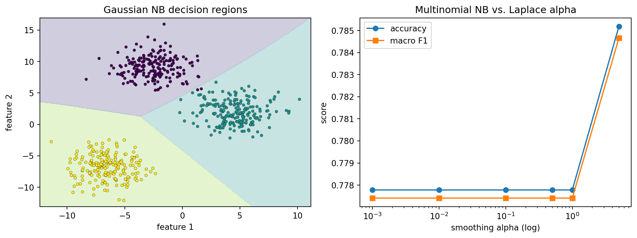
The example below makes the theory concrete with runnable code. It fits a Gaussian Naive Bayes model to a synthetic three-class problem and plots its decision regions, then trains a Multinomial Naive Bayes text classifier on a generated bag-of-words corpus while sweeping the Laplace pseudocount \(\alpha\), printing a results table of accuracy and macro F1. A short SymPy block symbolically confirms the posterior proportionality, the conditional independence log factorization, and that smoothing reduces to the maximum likelihood estimate as \(\alpha \to 0\). The Python tab runs here with a fixed seed; the Julia and Rust tabs are idiomatic illustrations of the same Gaussian Naive Bayes fit.
usingRandom, Statistics, PrintfRandom.seed!(42)# Three Gaussian blobs in 2D, one per class.functionmake_blobs(n, centers, sd) d =size(centers, 2) X =zeros(n *size(centers, 1), d) y =zeros(Int, n *size(centers, 1)) r =1for (c, mu) inenumerate(eachrow(centers))for _ in1:n X[r, :] = mu .+ sd .*randn(d) y[r] = c r +=1endendreturn X, yendcenters = [0.00.0; 6.06.0; -6.06.0]X, y =make_blobs(200, centers, 1.8)# Fit Gaussian NB: per-class mean, variance, and prior.classes =sort(unique(y))means =Dict(c =>vec(mean(X[y .== c, :], dims=1)) for c in classes)vars =Dict(c =>vec(var(X[y .== c, :], dims=1)) for c in classes)priors =Dict(c =>mean(y .== c) for c in classes)# Log Gaussian likelihood summed over independent features, plus log prior.functionlogscore(x, c) mu, v = means[c], vars[c] s =log(priors[c])for j ineachindex(x) s +=-0.5* (log(2pi * v[j]) + (x[j] - mu[j])^2/ v[j])endreturn sendpredict(x) = classes[argmax([logscore(x, c) for c in classes])]acc =mean(predict(X[i, :]) == y[i] for i in1:length(y))@printf("Gaussian NB training accuracy: %.3f\n", acc)
// Cargo.toml: rand = "0.8", rand_distr = "0.4"userand::{Rng, SeedableRng};userand::rngs::StdRng;userand_distr::StandardNormal;// Fit Gaussian NB and return per-class (mean, var, log_prior).fn fit(x:&[[f64;2]], y:&[usize], k:usize)->Vec<([f64;2], [f64;2],f64)>{let n = x.len() asf64; (0..k).map(|c|{let idx:Vec<usize>= (0..x.len()).filter(|&i| y[i] == c).collect();let m = idx.len() asf64;letmut mu = [0.0;2];for&i in&idx {for j in0..2{ mu[j] += x[i][j] / m;}}letmut var = [0.0;2];for&i in&idx {for j in0..2{ var[j] += (x[i][j] - mu[j]).powi(2) / m;}} (mu, var, (m / n).ln())}).collect()}fn log_score(xi:&[f64;2], p:&([f64;2], [f64;2],f64)) ->f64{let (mu, var, lp) = p;letmut s =*lp;for j in0..2{// Log Gaussian likelihood for independent feature j. s +=-0.5* ((2.0*std::f64::consts::PI * var[j]).ln()+ (xi[j] - mu[j]).powi(2) / var[j]);} s}fn main() {letmut rng =StdRng::seed_from_u64(42);let centers = [[0.0,0.0], [6.0,6.0], [-6.0,6.0]];letmut x =Vec::new();letmut y =Vec::new();for (c, ctr) in centers.iter().enumerate() {for _ in0..200{let a:f64= rng.sample(StandardNormal);let b:f64= rng.sample(StandardNormal); x.push([ctr[0] +1.8* a, ctr[1] +1.8* b]); y.push(c);}}let params = fit(&x,&y, centers.len());let correct = x.iter().zip(&y).filter(|(xi,&yi)|{let scores:Vec<f64>= params.iter().map(|p| log_score(xi, p)).collect();let pred = scores.iter().enumerate().max_by(|a, b| a.1.partial_cmp(b.1).unwrap()).unwrap().0; pred == yi}).count();println!("Gaussian NB training accuracy: {:.3}", correct asf64/ x.len() asf64);}
96.6.7 6.7 The Pipeline at a Glance
The diagram summarizes the flow from raw counts to a smoothed prediction.
flowchart TD
    A[Training data: features and labels] --> B[Estimate priors P of y from class frequencies]
    A --> C[Accumulate per-class feature counts]
    C --> D[Apply Laplace smoothing: add alpha to every count]
    D --> E[Store log likelihoods log P of x_j given y]
    B --> F[New input x]
    E --> F
    F --> G[Score each class: log prior plus sum of log likelihoods]
    G --> H[Predict argmax class]
    G --> I[Softmax of scores gives posterior probabilities]
96.7 7. Summary
Naive Bayes begins from the exact identity of Bayes’ theorem and then makes one bold simplification: features are conditionally independent given the class. This assumption reduces an intractable joint distribution to a product of simple univariate distributions, turns training into counting, and makes inference a sum of logarithms. The generative model it defines lets us classify by the MAP rule, choosing the class whose prior and likelihood best explain the data. Although the independence assumption is almost always false, the method works because correct classification needs only the right argmax, not accurate probabilities, and because the strong assumption acts as a regularizer that wins on variance in small data settings. Laplace smoothing completes the picture, replacing brittle zero probabilities with a principled Dirichlet posterior mean that keeps the model robust to unseen feature values. The result is a classifier that is fast, frugal with data, easy to implement, and a durable baseline across decades of machine learning practice.
96.8 References
Domingos, P., and Pazzani, M. “On the Optimality of the Simple Bayesian Classifier under Zero-One Loss.” Machine Learning, 1997. DOI: 10.1023/A:1007413511361. https://doi.org/10.1023/A:1007413511361
Rish, I. “An Empirical Study of the Naive Bayes Classifier.” IJCAI Workshop on Empirical Methods in AI, 2001. https://www.cc.gatech.edu/~isbell/reading/papers/Rish.pdf
Manning, C. D., Raghavan, P., and Schutze, H. “Introduction to Information Retrieval,” Chapter 13: Text Classification and Naive Bayes. Cambridge University Press, 2008. DOI: 10.1017/CBO9780511809071. https://doi.org/10.1017/CBO9780511809071
Ng, A. Y., and Jordan, M. I. “On Discriminative vs. Generative Classifiers: A Comparison of Logistic Regression and Naive Bayes.” NeurIPS, 2001. https://papers.nips.cc/paper/2020-on-discriminative-vs-generative-classifiers-a-comparison-of-logistic-regression-and-naive-bayes
Zhang, H. “The Optimality of Naive Bayes.” FLAIRS Conference, 2004. https://www.cs.unb.ca/~hzhang/publications/FLAIRS04ZhangH.pdf
Hastie, T., Tibshirani, R., and Friedman, J. “The Elements of Statistical Learning.” Springer, 2009. DOI: 10.1007/978-0-387-84858-7. https://doi.org/10.1007/978-0-387-84858-7
Lidstone, G. J. “Note on the General Case of the Bayes-Laplace Formula for Inductive or A Posteriori Probabilities.” Transactions of the Faculty of Actuaries, 1920. https://doi.org/10.1017/S2049221700004137
scikit-learn developers. “Naive Bayes.” scikit-learn User Guide. https://scikit-learn.org/stable/modules/naive_bayes.html
Source Code
# Naive Bayes TheoryNaive Bayes is one of the oldest and most enduring families of probabilistic classifiers. It is fast to train, requires little data relative to its discriminative cousins, and remains a strong baseline for text classification, spam filtering, and medical screening. Yet its theoretical foundation rests on an assumption that is almost always false: that features are conditionally independent given the class. This chapter develops the theory carefully, explains the generative model that gives Naive Bayes its name, derives the maximum a posteriori (MAP) decision rule, and confronts the central puzzle of the method, namely why a model built on a wildly inaccurate assumption so often classifies well. We close with Laplace smoothing, the practical fix that keeps the model from collapsing on unseen feature values.## 1. The Classification Problem and Bayes' Theorem### 1.1 Setup and NotationWe observe a feature vector $\mathbf{x} = (x_1, x_2, \dots, x_d)$ and wish to assign it to one of $K$ classes $y \in \{1, 2, \dots, K\}$. A probabilistic classifier models the relationship between $\mathbf{x}$ and $y$ through a joint or conditional distribution, then uses that model to predict the most probable class for a new input.The quantity we ultimately care about is the posterior probability $P(y \mid \mathbf{x})$, the probability of class $y$ given the observed features. If we knew this distribution exactly, the optimal strategy under zero-one loss would be to predict the class that maximizes it. The difficulty is that $P(y \mid \mathbf{x})$ is hard to estimate directly when $\mathbf{x}$ is high dimensional, because the number of distinct feature combinations grows exponentially with $d$.### 1.2 Bayes' TheoremBayes' theorem rewrites the posterior in terms of quantities that are often easier to estimate:$$P(y \mid \mathbf{x}) = \frac{P(\mathbf{x} \mid y)\, P(y)}{P(\mathbf{x})}.$$Here $P(y)$ is the prior probability of the class, $P(\mathbf{x} \mid y)$ is the class conditional likelihood of the features, and $P(\mathbf{x})$ is the marginal probability of the data, sometimes called the evidence. The evidence does not depend on $y$, so for the purpose of choosing a class we may ignore it and work with the unnormalized posterior:$$P(y \mid \mathbf{x}) \propto P(\mathbf{x} \mid y)\, P(y).$$This identity is exact. The trouble begins when we try to estimate $P(\mathbf{x} \mid y)$. In full generality this is a joint distribution over $d$ variables, and estimating it reliably from a finite sample is hopeless without further structure. Naive Bayes supplies that structure through a single strong assumption.## 2. The Conditional Independence Assumption### 2.1 Statement of the AssumptionThe naive assumption is that, given the class label, the features are mutually independent. Formally, for all classes $y$ and all feature vectors,$$P(\mathbf{x} \mid y) = P(x_1, x_2, \dots, x_d \mid y) = \prod_{j=1}^{d} P(x_j \mid y).$$In words, once we know the class, learning the value of one feature tells us nothing about the value of any other. This is what the word "naive" refers to. It is rarely true in any literal sense. In a document, the appearance of the word "San" makes "Francisco" far more likely whether or not we already know the topic. The assumption ignores all such correlations.### 2.2 Why the Assumption Is So PowerfulThe payoff for accepting this falsehood is enormous. Without it, we would need to estimate a joint distribution whose parameter count grows exponentially in $d$. With it, we only need the $d$ univariate distributions $P(x_j \mid y)$, one per feature per class. The parameter count becomes linear in $d$.Consider binary features. Modeling the full joint $P(\mathbf{x} \mid y)$ for one class requires $2^d - 1$ parameters. Under conditional independence, it requires only $d$ parameters, one Bernoulli probability per feature. For $d = 1000$, the difference is between an astronomical $2^{1000}$ and a manageable $1000$. This collapse in complexity is the entire reason Naive Bayes can be trained on small datasets and run at scale.### 2.3 Conditional Versus Marginal IndependenceA frequent point of confusion deserves emphasis. The assumption is one of conditional independence given the class, not marginal independence. Features may be strongly correlated overall while still being approximately independent within each class. Height and vocabulary size are correlated in the general population because children are both shorter and less verbal. Conditioned on age, the correlation largely vanishes. Naive Bayes only requires that the within-class correlations be weak, which is a much milder demand than full independence.## 3. The Generative Model### 3.1 A Story for How Data Is ProducedNaive Bayes is a generative classifier. Rather than modeling the boundary between classes directly, it models how the data in each class is generated, then inverts that model with Bayes' theorem. The generative story is simple:1. Draw a class label $y$ from the prior distribution $P(y)$.2. Given that label, draw each feature $x_j$ independently from its class conditional distribution $P(x_j \mid y)$.The joint distribution implied by this story is$$P(y, \mathbf{x}) = P(y) \prod_{j=1}^{d} P(x_j \mid y).$$Any sample from the model is produced by first selecting a class, then sampling each coordinate on its own. Because the model specifies a full joint distribution over labels and features, we could in principle use it to generate synthetic examples, not merely to classify. That is the defining property of a generative model, as opposed to a discriminative model such as logistic regression, which models $P(y \mid \mathbf{x})$ directly and cannot generate features.### 3.2 Choosing the Feature DistributionThe factor $P(x_j \mid y)$ must be given a parametric form suited to the data. Three common choices define the standard Naive Bayes variants.**Gaussian Naive Bayes** is used for continuous features. Each $P(x_j \mid y)$ is modeled as a normal distribution with a class specific mean and variance:$$P(x_j \mid y) = \frac{1}{\sqrt{2\pi \sigma_{jy}^2}} \exp\!\left(-\frac{(x_j - \mu_{jy})^2}{2\sigma_{jy}^2}\right).$$**Multinomial Naive Bayes** is the workhorse for text classification with word counts. The features represent counts of events, and the class conditional is a multinomial distribution over the vocabulary. The probability that word $w$ occurs in class $y$ is a parameter $\theta_{wy}$, with $\sum_w \theta_{wy} = 1$.**Bernoulli Naive Bayes** models binary features, such as the presence or absence of each word, with a Bernoulli distribution per feature.The model structure stays the same across all three; only the form of $P(x_j \mid y)$ changes.### 3.3 Maximum Likelihood Parameter EstimationTraining a Naive Bayes model means estimating the prior $P(y)$ and the class conditionals $P(x_j \mid y)$. Because the log likelihood factors over classes and features, the maximum likelihood estimates are simple counts and averages computed independently.The prior is the empirical class frequency. If $N_y$ examples out of $N$ belong to class $y$, then$$\hat{P}(y) = \frac{N_y}{N}.$$For multinomial features, the class conditional probability of word $w$ is the fraction of all word occurrences in class $y$ documents that are the word $w$:$$\hat{\theta}_{wy} = \frac{N_{wy}}{\sum_{w'} N_{w'y}},$$where $N_{wy}$ is the total count of word $w$ across documents of class $y$. For Gaussian features, the estimates are the per class sample mean and variance of each feature. No iterative optimization is required. Training amounts to a single pass over the data to accumulate counts, which is why Naive Bayes is among the fastest classifiers to fit.## 4. MAP Classification### 4.1 The Decision RuleGiven the trained model and a new input $\mathbf{x}$, we predict the class with the largest posterior probability. This is the maximum a posteriori, or MAP, estimate:$$\hat{y} = \arg\max_{y} P(y \mid \mathbf{x}) = \arg\max_{y} P(y) \prod_{j=1}^{d} P(x_j \mid y).$$The MAP rule combines the prior belief about each class with the evidence supplied by the features. When the prior is uniform, meaning all classes are equally likely a priori, MAP reduces to maximum likelihood classification, in which we pick the class whose conditional likelihood best explains the observed features.It is worth assembling the full chain of reasoning in one place, since every step is either an exact identity or the single naive assumption. Starting from the definition of the posterior and applying Bayes' theorem, the conditional independence factorization, and the fact that the evidence is constant in $y$, we obtain$$\begin{aligned}\hat{y}&= \arg\max_{y} \; P(y \mid \mathbf{x})&&\text{(MAP objective)} \\&= \arg\max_{y} \; \frac{P(\mathbf{x} \mid y)\, P(y)}{P(\mathbf{x})}&&\text{(Bayes' theorem)} \\&= \arg\max_{y} \; P(\mathbf{x} \mid y)\, P(y)&&\text{(drop evidence }P(\mathbf{x})\text{)} \\&= \arg\max_{y} \; P(y) \prod_{j=1}^{d} P(x_j \mid y)&&\text{(conditional independence)} \\&= \arg\max_{y} \left[ \log P(y) + \sum_{j=1}^{d} \log P(x_j \mid y) \right].&&\text{(monotone }\log\text{)}\end{aligned}$$Only the fourth line uses an approximation; the rest are exact. This makes precise where the model's strength and its fragility both live: a single factorization step buys the entire reduction in complexity, and any error the method commits enters through that one line.### 4.2 Working in Log SpaceThe product of many probabilities, each less than one, quickly underflows to zero in floating point arithmetic. For a document with hundreds of words, $\prod_j P(x_j \mid y)$ may be smaller than the smallest representable positive number. The standard remedy is to maximize the logarithm of the posterior, which turns the product into a sum and is monotonic so it does not change the arg max:$$\hat{y} = \arg\max_{y} \left[ \log P(y) + \sum_{j=1}^{d} \log P(x_j \mid y) \right].$$This log sum is numerically stable and also faster, since addition is cheaper than multiplication. Every practical implementation computes scores this way.```python# Scoring a single example under a trained multinomial model.# log_prior[y] and log_likelihood[y][w] are precomputed during training.def predict(features, classes, log_prior, log_likelihood): best_class, best_score =None, float("-inf")for y in classes: score = log_prior[y]for w, count in features.items(): score += count * log_likelihood[y][w]if score > best_score: best_class, best_score = y, scorereturn best_class```### 4.3 Recovering Calibrated ProbabilitiesIf we want an actual probability rather than only the winning class, we normalize the exponentiated log scores. Letting $s_y$ denote the log posterior score for class $y$, the normalized posterior is$$P(y \mid \mathbf{x}) = \frac{\exp(s_y)}{\sum_{k} \exp(s_k)}.$$This is the softmax of the log scores. A practical caution applies here. The probabilities Naive Bayes produces are often poorly calibrated and tend toward zero or one, a side effect of the independence assumption treating correlated features as independent pieces of evidence. We return to this in the next section. The point class predictions can remain excellent even when these probability estimates are unreliable.## 5. Why It Works Despite the Strong Assumption### 5.1 Classification Needs the Argmax, Not the ProbabilityThe resolution to the central puzzle is that classification under zero-one loss requires only that the correct class receive the highest posterior score, not that the scores themselves be accurate. The independence assumption can badly distort the magnitude of $P(y \mid \mathbf{x})$ while leaving the ranking of classes intact. As long as the distortions do not flip which class is on top, the classifier is correct.A useful way to see this is to consider the decision boundary. For two classes, we predict class 1 when$$\log \frac{P(y=1 \mid \mathbf{x})}{P(y=2 \mid \mathbf{x})} > 0.$$Errors in the estimated log ratio that do not change its sign do not change any decision. Naive Bayes can be confidently wrong about the numeric posterior and still draw the boundary in nearly the right place.### 5.2 The Effect of Dependence on the Optimal BoundaryDomingos and Pazzani gave a careful analysis showing that Naive Bayes is optimal under conditions far broader than independence. They proved that the classifier achieves the Bayes optimal decision for any concept that is a disjunction or conjunction of features, even though such concepts violate independence. The key insight is that feature dependence harms accuracy only when it pushes the estimated posterior across the decision boundary. Much of the time the dependence shifts both class scores in the same direction and the boundary is preserved.When features are duplicated or correlated, Naive Bayes does double count the evidence, which inflates confidence and skews the posterior toward the extremes. This is exactly why calibration suffers. But the inflation often affects the competing classes in a way that does not reverse their order, so the final label is unchanged. The model is, in the memorable phrase, a good classifier but a poor estimator of probability.### 5.3 Bias and VarianceThere is also a statistical reason for the method's robustness. By imposing strong structure, Naive Bayes is a high bias, low variance estimator. It cannot represent feature interactions, which is a source of bias, but its few parameters are each estimated from a large effective sample, which keeps variance low. In small data regimes, where a more flexible model would overfit and suffer high variance, the low variance of Naive Bayes wins on overall error. The independence assumption acts as a powerful regularizer. This is why Naive Bayes frequently outperforms more expressive classifiers when training data is scarce, and why it remains a sensible first baseline.### 5.4 When It FailsThe honest converse is that Naive Bayes fails when feature dependencies are strong and aligned in a way that does flip the decision, when accurate probability estimates are needed for downstream cost sensitive decisions, or when the chosen parametric form for $P(x_j \mid y)$ is a poor fit for the data. Recognizing these failure modes matters as much as appreciating the method's strengths.## 6. Laplace Smoothing### 6.1 The Zero Frequency ProblemA maximum likelihood estimate assigns probability zero to any feature value never seen with a given class during training. Suppose the word "transformer" never appeared in any training document labeled as sports. Then $\hat{\theta}_{\text{transformer},\,\text{sports}} = 0$. When a test document contains that word, the entire product for the sports class becomes zero, regardless of how strongly every other word points to sports. A single unseen word vetoes the class. In log space, this is the equally fatal $\log 0 = -\infty$.This is not a rare edge case. Real vocabularies are large, training data is finite, and the absence of a particular word from a particular class is common. The maximum likelihood estimate is too confident in declaring something impossible merely because it was unobserved.### 6.2 Additive SmoothingLaplace smoothing, also called additive smoothing, fixes this by adding a small pseudocount $\alpha > 0$ to every count before normalizing. For multinomial Naive Bayes over a vocabulary of size $V$, the smoothed estimate is$$\hat{\theta}_{wy} = \frac{N_{wy} + \alpha}{\sum_{w'} \left( N_{w'y} + \alpha \right)} = \frac{N_{wy} + \alpha}{\left(\sum_{w'} N_{w'y}\right) + \alpha V}.$$Setting $\alpha = 1$ recovers the original Laplace rule, which corresponds to having seen every word once in every class before looking at the data. Smaller values such as $\alpha = 0.1$, often called Lidstone smoothing, smooth less aggressively. With smoothing, every probability is strictly positive, so no single feature can zero out a class, and log space scoring never encounters $\log 0$.### 6.3 A Bayesian InterpretationAdditive smoothing is not an arbitrary hack. It is the posterior mean of the multinomial parameters under a symmetric Dirichlet prior with concentration parameter $\alpha$. The Dirichlet is the conjugate prior for the multinomial, so combining a $\text{Dirichlet}(\alpha, \dots, \alpha)$ prior with observed counts yields a Dirichlet posterior whose mean is exactly the smoothed estimate above. From this view, $\alpha$ encodes a prior belief that all feature values are possible, and the data updates that belief. The name "Naive Bayes" earns its Bayesian credentials most clearly here: the pseudocount is a genuine prior, and the smoothed estimate is a genuine posterior.### 6.4 Choosing the Smoothing StrengthThe pseudocount $\alpha$ is a hyperparameter, and its value trades off two failure modes. Too small, and rare but informative features can still dominate or contribute noise. Too large, and the estimates are pulled toward the uniform distribution, washing out the signal the features carry and increasing bias. In practice $\alpha$ is selected by cross validation, with $\alpha = 1$ a reasonable default and smaller values often preferred for large vocabularies where the additive mass $\alpha V$ would otherwise overwhelm modest counts.```python# Smoothed multinomial training: counts -> log likelihoods.import mathdef train_loglik(word_counts, vocab, alpha=1.0):# word_counts[y][w] is the count of word w in class y. log_likelihood = {} V =len(vocab)for y, counts in word_counts.items(): total =sum(counts.values()) + alpha * V log_likelihood[y] = { w: math.log((counts.get(w, 0) + alpha) / total)for w in vocab }return log_likelihood```### 6.5 A Worked Example End to EndA small numeric example ties the pieces together. Suppose we classify one-sentence messages as $\text{spam}$ or $\text{ham}$ with a vocabulary of three words, $V = \{\text{free}, \text{money}, \text{lunch}\}$. The training set has six spam and six ham messages. Pooling word counts within each class gives the totals in the table.| count | free | money | lunch | class total ||-------|------|-------|-------|-------------|| spam | 8 | 6 | 0 | 14 || ham | 1 | 2 | 9 | 12 |The priors are equal, $\hat{P}(\text{spam}) = \hat{P}(\text{ham}) = \tfrac{6}{12} = 0.5$. Now classify the new message "free lunch", that is the count vector with one occurrence each of "free" and "lunch". The raw maximum likelihood estimate gives $\hat{\theta}_{\text{lunch}, \text{spam}} = 0/14 = 0$, so the spam score collapses to zero no matter how strongly "free" leans spam. This is the zero frequency problem in action.Apply Laplace smoothing with $\alpha = 1$ and $V = 3$. The smoothed likelihoods for the two relevant words are$$\hat{\theta}_{\text{free}, \text{spam}} = \frac{8 + 1}{14 + 3} = \frac{9}{17}, \qquad\hat{\theta}_{\text{lunch}, \text{spam}} = \frac{0 + 1}{14 + 3} = \frac{1}{17},$$$$\hat{\theta}_{\text{free}, \text{ham}} = \frac{1 + 1}{12 + 3} = \frac{2}{15}, \qquad\hat{\theta}_{\text{lunch}, \text{ham}} = \frac{9 + 1}{12 + 3} = \frac{10}{15}.$$The log posterior scores, up to the shared evidence term, are$$\begin{aligned}s_{\text{spam}} &= \log 0.5 + \log \tfrac{9}{17} + \log \tfrac{1}{17} \approx -0.693 - 0.636 - 2.833 = -4.162, \\s_{\text{ham}} &= \log 0.5 + \log \tfrac{2}{15} + \log \tfrac{10}{15} \approx -0.693 - 2.015 - 0.405 = -3.113.\end{aligned}$$Since $s_{\text{ham}} > s_{\text{spam}}$, the message is classified as ham, driven by the decisive "lunch" evidence. Normalizing with the softmax of section 4.3 gives $P(\text{ham} \mid \mathbf{x}) = \tfrac{e^{s_{\text{ham}}}}{e^{s_{\text{spam}}} + e^{s_{\text{ham}}}} \approx 0.74$. Without smoothing the spam score would have been $-\infty$, an unwarranted certainty produced by one unobserved word. The smoothed model reaches a sensible, finite decision.### 6.6 Computational IllustrationThe example below makes the theory concrete with runnable code. It fits a Gaussian Naive Bayes model to a synthetic three-class problem and plots its decision regions, then trains a Multinomial Naive Bayes text classifier on a generated bag-of-words corpus while sweeping the Laplace pseudocount $\alpha$, printing a results table of accuracy and macro F1. A short SymPy block symbolically confirms the posterior proportionality, the conditional independence log factorization, and that smoothing reduces to the maximum likelihood estimate as $\alpha \to 0$. The Python tab runs here with a fixed seed; the Julia and Rust tabs are idiomatic illustrations of the same Gaussian Naive Bayes fit.::: {.panel-tabset}## Python```{python}import numpy as npimport pandas as pdimport matplotlib.pyplot as pltimport sympy as spfrom sklearn.datasets import make_blobsfrom sklearn.naive_bayes import GaussianNB, MultinomialNBfrom sklearn.metrics import accuracy_score, f1_scorefrom sklearn.model_selection import train_test_splitrng = np.random.default_rng(42)# --- SymPy: posterior proportionality and smoothing as Dirichlet mean ---Px_given_y, Py, Px = sp.symbols("P_x_given_y P_y P_x", positive=True)print("posterior * P(x) =", sp.simplify((Px_given_y * Py / Px) * Px)," (= P(x|y) P(y))")p1, p2, p3, pri = sp.symbols("p1 p2 p3 pi_y", positive=True)print("log P(y, x) =", sp.expand_log(sp.log(pri * p1 * p2 * p3), force=True))N_wy, total, a, V = sp.symbols("N_wy N_total alpha V", positive=True)smoothed = (N_wy + a) / (total + a * V)print("smoothed theta =", smoothed, " limit(alpha->0) =", sp.limit(smoothed, a, 0))# --- Gaussian NB decision boundary on three blobs ---X, y = make_blobs(n_samples=600, centers=3, cluster_std=1.8, random_state=42)gnb = GaussianNB().fit(X, y)xx, yy = np.meshgrid( np.linspace(X[:, 0].min() -1, X[:, 0].max() +1, 300), np.linspace(X[:, 1].min() -1, X[:, 1].max() +1, 300),)Z = gnb.predict(np.c_[xx.ravel(), yy.ravel()]).reshape(xx.shape)print(f"\nGaussian NB training accuracy: "f"{accuracy_score(y, gnb.predict(X)):.3f}")# --- Synthetic bag-of-words corpus: three overlapping topics ---vocab_size, n_topics, docs_per_topic =60, 3, 300topic_word = np.full((n_topics, vocab_size), 1.0)for t inrange(n_topics): topic_word[t, t *16: t *16+22] +=1.5topic_word /= topic_word.sum(axis=1, keepdims=True)X_txt, y_txt = [], []for t inrange(n_topics):for _ inrange(docs_per_topic): length = rng.integers(8, 18) # short, noisy documents X_txt.append(rng.multinomial(length, topic_word[t])) y_txt.append(t)X_txt, y_txt = np.array(X_txt), np.array(y_txt)Xtr, Xte, ytr, yte = train_test_split( X_txt, y_txt, test_size=0.3, random_state=42, stratify=y_txt)# --- Multinomial NB: sweep the Laplace pseudocount ---rows = []for alpha in [0.001, 0.01, 0.1, 0.5, 1.0, 5.0]: clf = MultinomialNB(alpha=alpha).fit(Xtr, ytr) pred = clf.predict(Xte) rows.append({"alpha": alpha,"test_accuracy": accuracy_score(yte, pred),"macro_f1": f1_score(yte, pred, average="macro")})results = pd.DataFrame(rows)print("\nMultinomial NB: Laplace smoothing sweep (synthetic 3-topic corpus)")print(results.to_string(index=False, float_format=lambda v: f"{v:0.4f}"))# --- Figures ---fig, ax = plt.subplots(1, 2, figsize=(11, 4.2))ax[0].contourf(xx, yy, Z, alpha=0.25, cmap="viridis", levels=2)ax[0].scatter(X[:, 0], X[:, 1], c=y, s=12, cmap="viridis", edgecolor="k", linewidth=0.2)ax[0].set_title("Gaussian NB decision regions")ax[0].set_xlabel("feature 1"); ax[0].set_ylabel("feature 2")ax[1].plot(results["alpha"], results["test_accuracy"], marker="o", label="accuracy")ax[1].plot(results["alpha"], results["macro_f1"], marker="s", label="macro F1")ax[1].set_xscale("log")ax[1].set_title("Multinomial NB vs. Laplace alpha")ax[1].set_xlabel("smoothing alpha (log)"); ax[1].set_ylabel("score")ax[1].legend()fig.tight_layout()plt.show()```## Julia```juliausingRandom, Statistics, PrintfRandom.seed!(42)# Three Gaussian blobs in 2D, one per class.functionmake_blobs(n, centers, sd) d =size(centers, 2) X =zeros(n *size(centers, 1), d) y =zeros(Int, n *size(centers, 1)) r =1for (c, mu) inenumerate(eachrow(centers))for _ in1:n X[r, :] = mu .+ sd .*randn(d) y[r] = c r +=1endendreturn X, yendcenters = [0.00.0; 6.06.0; -6.06.0]X, y =make_blobs(200, centers, 1.8)# Fit Gaussian NB: per-class mean, variance, and prior.classes =sort(unique(y))means =Dict(c =>vec(mean(X[y .== c, :], dims=1)) for c in classes)vars =Dict(c =>vec(var(X[y .== c, :], dims=1)) for c in classes)priors =Dict(c =>mean(y .== c) for c in classes)# Log Gaussian likelihood summed over independent features, plus log prior.functionlogscore(x, c) mu, v = means[c], vars[c] s =log(priors[c])for j ineachindex(x) s +=-0.5* (log(2pi * v[j]) + (x[j] - mu[j])^2/ v[j])endreturn sendpredict(x) = classes[argmax([logscore(x, c) for c in classes])]acc =mean(predict(X[i, :]) == y[i] for i in1:length(y))@printf("Gaussian NB training accuracy: %.3f\n", acc)```## Rust```rust// Cargo.toml: rand ="0.8", rand_distr ="0.4"use rand::{Rng, SeedableRng};use rand::rngs::StdRng;use rand_distr::StandardNormal;// Fit Gaussian NB and return per-class (mean, var, log_prior).fn fit(x:&[[f64; 2]], y:&[usize], k: usize)->Vec<([f64; 2], [f64; 2], f64)> {let n = x.len() as f64; (0..k).map(|c| {let idx: Vec<usize>= (0..x.len()).filter(|&i| y[i] == c).collect();let m = idx.len() as f64;let mut mu = [0.0; 2];for&i in&idx { for j in0..2 { mu[j] += x[i][j] / m; } }let mut var = [0.0; 2];for&i in&idx { for j in0..2 { var[j] += (x[i][j] - mu[j]).powi(2) / m; } } (mu, var, (m / n).ln()) }).collect()}fn log_score(xi:&[f64; 2], p:&([f64; 2], [f64; 2], f64)) -> f64 {let (mu, var, lp) = p;let mut s =*lp;for j in0..2 {// Log Gaussian likelihood for independent feature j. s +=-0.5* ((2.0* std::f64::consts::PI * var[j]).ln()+ (xi[j] - mu[j]).powi(2) / var[j]); } s}fn main() {let mut rng = StdRng::seed_from_u64(42);let centers = [[0.0, 0.0], [6.0, 6.0], [-6.0, 6.0]];let mut x = Vec::new();let mut y = Vec::new();for (c, ctr) in centers.iter().enumerate() {for _ in0..200 {let a: f64 = rng.sample(StandardNormal);let b: f64 = rng.sample(StandardNormal); x.push([ctr[0] +1.8* a, ctr[1] +1.8* b]); y.push(c); } }let params =fit(&x, &y, centers.len());let correct = x.iter().zip(&y).filter(|(xi, &yi)| {let scores: Vec<f64>= params.iter().map(|p|log_score(xi, p)).collect();let pred = scores.iter().enumerate() .max_by(|a, b| a.1.partial_cmp(b.1).unwrap()).unwrap().0; pred == yi }).count();println!("Gaussian NB training accuracy: {:.3}", correct as f64 / x.len() as f64);}```:::### 6.7 The Pipeline at a GlanceThe diagram summarizes the flow from raw counts to a smoothed prediction.```{mermaid}flowchart TD A[Training data: features and labels] --> B[Estimate priors P of y from class frequencies] A --> C[Accumulate per-class feature counts] C --> D[Apply Laplace smoothing: add alpha to every count] D --> E[Store log likelihoods log P of x_j given y] B --> F[New input x] E --> F F --> G[Score each class: log prior plus sum of log likelihoods] G --> H[Predict argmax class] G --> I[Softmax of scores gives posterior probabilities]```## 7. SummaryNaive Bayes begins from the exact identity of Bayes' theorem and then makes one bold simplification: features are conditionally independent given the class. This assumption reduces an intractable joint distribution to a product of simple univariate distributions, turns training into counting, and makes inference a sum of logarithms. The generative model it defines lets us classify by the MAP rule, choosing the class whose prior and likelihood best explain the data. Although the independence assumption is almost always false, the method works because correct classification needs only the right argmax, not accurate probabilities, and because the strong assumption acts as a regularizer that wins on variance in small data settings. Laplace smoothing completes the picture, replacing brittle zero probabilities with a principled Dirichlet posterior mean that keeps the model robust to unseen feature values. The result is a classifier that is fast, frugal with data, easy to implement, and a durable baseline across decades of machine learning practice.## References1. Domingos, P., and Pazzani, M. "On the Optimality of the Simple Bayesian Classifier under Zero-One Loss." Machine Learning, 1997. DOI: 10.1023/A:1007413511361. https://doi.org/10.1023/A:10074135113612. Rish, I. "An Empirical Study of the Naive Bayes Classifier." IJCAI Workshop on Empirical Methods in AI, 2001. https://www.cc.gatech.edu/~isbell/reading/papers/Rish.pdf3. Manning, C. D., Raghavan, P., and Schutze, H. "Introduction to Information Retrieval," Chapter 13: Text Classification and Naive Bayes. Cambridge University Press, 2008. DOI: 10.1017/CBO9780511809071. https://doi.org/10.1017/CBO97805118090714. Ng, A. Y., and Jordan, M. I. "On Discriminative vs. Generative Classifiers: A Comparison of Logistic Regression and Naive Bayes." NeurIPS, 2001. https://papers.nips.cc/paper/2020-on-discriminative-vs-generative-classifiers-a-comparison-of-logistic-regression-and-naive-bayes5. Zhang, H. "The Optimality of Naive Bayes." FLAIRS Conference, 2004. https://www.cs.unb.ca/~hzhang/publications/FLAIRS04ZhangH.pdf6. Hastie, T., Tibshirani, R., and Friedman, J. "The Elements of Statistical Learning." Springer, 2009. DOI: 10.1007/978-0-387-84858-7. https://doi.org/10.1007/978-0-387-84858-77. Lidstone, G. J. "Note on the General Case of the Bayes-Laplace Formula for Inductive or A Posteriori Probabilities." Transactions of the Faculty of Actuaries, 1920. https://doi.org/10.1017/S20492217000041378. scikit-learn developers. "Naive Bayes." scikit-learn User Guide. https://scikit-learn.org/stable/modules/naive_bayes.html