Gaussian mixture models (GMMs) sit at the crossroads of clustering, density estimation, and probabilistic modeling. Where \(k\)-means partitions data into disjoint groups by minimizing within cluster distance, a GMM treats the data as samples from a weighted sum of Gaussian densities and infers both the parameters of those densities and the probability that each point belongs to each component. This probabilistic stance buys us soft assignments, a principled likelihood we can optimize and compare, and a generative story that explains how the observed data could have been produced. The price is a nonconvex objective, sensitivity to initialization, and a handful of numerical hazards that a careful practitioner must manage. This chapter develops the model from its latent variable foundations, derives the soft assignment and likelihood machinery, surveys the covariance parameterizations that control model complexity, and closes with model selection by the Bayesian information criterion.
134.1 1. The Generative Model
A Gaussian mixture model assumes that each observation \(\mathbf{x} \in \mathbb{R}^d\) is drawn from one of \(K\) Gaussian components, but we do not observe which one. The density is a convex combination of component densities:
where \(\pi_k\) are the mixing weights satisfying \(\pi_k \geq 0\) and \(\sum_{k=1}^{K} \pi_k = 1\), and each \(\mathcal{N}(\mathbf{x} \mid \boldsymbol{\mu}_k, \boldsymbol{\Sigma}_k)\) is a multivariate Gaussian with mean \(\boldsymbol{\mu}_k\) and covariance \(\boldsymbol{\Sigma}_k\). The full parameter set is \(\boldsymbol{\theta} = \{\pi_k, \boldsymbol{\mu}_k, \boldsymbol{\Sigma}_k\}_{k=1}^{K}\). The multivariate Gaussian density is
The mixture is far more expressive than a single Gaussian. With enough components a GMM can approximate any smooth density to arbitrary accuracy, which makes it a workhorse for density estimation as well as clustering. The model is also generative in a literal sense: to sample a point, first draw a component index from the categorical distribution over \(\{1, \dots, K\}\) with probabilities \(\pi_k\), then draw \(\mathbf{x}\) from the chosen Gaussian.
134.2 2. The Latent Variable Formulation
The clean way to reason about a GMM is to make the unobserved component identity explicit. Introduce a latent variable \(\mathbf{z} \in \{0,1\}^K\) for each observation, a one hot vector in which \(z_k = 1\) indicates that the point was generated by component \(k\). The latent variable follows a categorical prior:
This formulation is not just notational hygiene. The latent variable is exactly what the expectation maximization (EM) algorithm reasons about, and the posterior over \(\mathbf{z}\) given \(\mathbf{x}\) is precisely the soft assignment we develop next.
134.3 3. Soft Assignments and Responsibilities
The quantity that distinguishes a GMM from hard clustering is the posterior probability that a given point belongs to each component. Applying Bayes’ rule to the latent variable yields the responsibility:
The numerator is the joint probability that component \(k\) generated the point, and the denominator is the marginal evidence \(p(\mathbf{x}_n)\) that normalizes across components. By construction \(\sum_{k=1}^{K} \gamma(z_{nk}) = 1\), so each point distributes one unit of membership across the components in proportion to how well each explains it.
This soft assignment is the substantive difference from \(k\)-means. A point sitting between two clusters might receive responsibilities of \(0.55\) and \(0.45\), honestly reflecting ambiguity rather than forcing a binary choice. In fact \(k\)-means is recoverable as a limiting case: fix every covariance to \(\sigma^2 \mathbf{I}\), hold the mixing weights equal, and let \(\sigma^2 \to 0\). The responsibilities then collapse onto the nearest centroid, and EM reduces to Lloyd’s algorithm. The GMM is therefore a strict generalization that relaxes the equal isotropic variance assumption and the hard assignment.
Responsibilities also drive the parameter updates. Define the effective number of points assigned to component \(k\) as \(N_k = \sum_{n=1}^{N} \gamma(z_{nk})\). The EM maximization step then produces closed form updates that are responsibility weighted versions of the ordinary sample statistics:
Each component’s mean is the weighted centroid of the data, its covariance is the weighted scatter, and its mixing weight is the fraction of total responsibility it captured. The expectation step recomputes the responsibilities from the current parameters, and the two steps alternate until convergence.
The pseudocode below summarizes a single EM pass. The E-step recomputes responsibilities from the current parameters, and the M-step updates the parameters from those responsibilities, repeating until the log likelihood change falls below a tolerance.
EM for a GMM (one pass)
  E-step: for each n, k compute gamma(z_nk) from current params
  M-step: N_k   = sum_n gamma(z_nk)
          mu_k  = (1/N_k) sum_n gamma(z_nk) x_n
          Sig_k = (1/N_k) sum_n gamma(z_nk) (x_n - mu_k)(x_n - mu_k)^T
          pi_k  = N_k / N
  repeat until log-likelihood change < tol
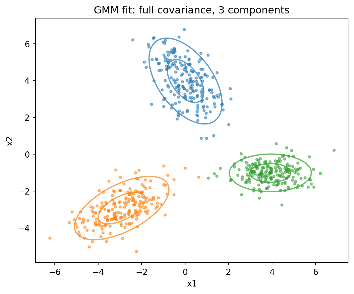
The following cell fits a three component GMM with full covariances to synthetic data and draws each fitted component as one and two standard deviation ellipses, illustrating the elliptical, rotated shapes that full covariances capture. The fitted means, covariances, and mixing weights are exactly the responsibility weighted statistics from the M-step above.
The responsibilities are the soft assignments derived above. Each row sums to one, distributing a single unit of membership across the components in proportion to how well each explains the point.
Code
resp = gmm.predict_proba(X)np.set_printoptions(precision=3, suppress=True)for i in [0, 250, 450]:print(f"point {i}: responsibilities = {resp[i]}, sum = {resp[i].sum():.3f}")
point 0: responsibilities = [0. 1. 0.], sum = 1.000
point 250: responsibilities = [1. 0. 0.], sum = 1.000
point 450: responsibilities = [0. 0. 1.], sum = 1.000
134.4 4. The Likelihood
Given \(N\) independent observations \(\mathbf{X} = \{\mathbf{x}_1, \dots, \mathbf{x}_N\}\), the parameters are fit by maximizing the log likelihood:
The sum inside the logarithm is the source of every difficulty. Because the log cannot be pushed through the sum, the objective does not factor into per component terms and there is no closed form maximizer. The function is also nonconvex, with multiple local optima and saddle points, so the solution returned by EM depends on initialization. Standard practice is to run EM from several random restarts, or from a \(k\)-means initialization, and keep the run with the highest likelihood.
EM optimizes this objective indirectly. It is guaranteed to increase the log likelihood at every iteration, or leave it unchanged at a stationary point, which follows from the fact that EM maximizes a variational lower bound that touches the true likelihood after each E-step. This monotone ascent property makes EM numerically stable and easy to monitor: track the log likelihood and stop when its increase falls below a tolerance.
Two failure modes deserve attention. First, the likelihood is unbounded. If a component’s mean coincides with a single data point and its covariance shrinks toward zero, that component’s density at the point diverges and the likelihood goes to infinity. These singular solutions are degenerate and must be guarded against, typically by adding a small ridge \(\varepsilon \mathbf{I}\) to each covariance (a maximum a posteriori regularization with an inverse Wishart prior) or by resetting any component whose effective count \(N_k\) collapses. Second, the likelihood is invariant to relabeling the components. Any permutation of the \(K\) labels gives an identical likelihood, so there are \(K!\) equivalent optima. This label switching is harmless for clustering and density estimation but matters if one tries to interpret individual component parameters across runs.
In practice the per point density should be computed in log space using the log-sum-exp trick to avoid underflow when the exponentials are tiny:
The Cholesky factorization serves double duty: it gives a numerically stable route to both the quadratic form and the log determinant, and it fails fast if a covariance has lost positive definiteness, which is a useful early warning of a collapsing component.
134.5 5. Covariance Types
The covariance parameterization is the main lever for controlling a GMM’s flexibility and its parameter count. Richer covariances capture correlated, elongated, or rotated clusters but demand more data and more compute. Four standard choices span the spectrum.
134.5.1 5.1 Full Covariance
Each component carries its own unrestricted symmetric positive definite matrix \(\boldsymbol{\Sigma}_k\). This is the most expressive option: components can be elongated and oriented arbitrarily, capturing any correlation structure among the \(d\) dimensions. Each covariance has \(d(d+1)/2\) free parameters, so the total scales as \(K \cdot d(d+1)/2\), which grows quadratically in dimension. Full covariances are appropriate when clusters are genuinely correlated and data is plentiful relative to \(d\).
134.5.2 5.2 Tied Covariance
All components share a single covariance matrix \(\boldsymbol{\Sigma}\), so they differ only in location. This encodes the assumption that every cluster has the same shape and orientation, an assumption identical to the one underlying linear discriminant analysis. It costs only \(d(d+1)/2\) covariance parameters in total regardless of \(K\), which is a strong regularizer when components are few or data is scarce.
134.5.3 5.3 Diagonal Covariance
Each component has a diagonal covariance, \(\boldsymbol{\Sigma}_k = \mathrm{diag}(\sigma_{k1}^2, \dots, \sigma_{kd}^2)\). This assumes the features are uncorrelated within each component, so the Gaussians are axis aligned ellipsoids that can stretch differently along each dimension but cannot rotate. The cost is only \(d\) parameters per component. Diagonal covariances are the default in high dimensional settings such as speaker recognition, where full covariances would be statistically and computationally prohibitive.
134.5.4 5.4 Spherical Covariance
The most constrained option sets \(\boldsymbol{\Sigma}_k = \sigma_k^2 \mathbf{I}\), a single scalar variance per component. Each cluster is a sphere that can vary in size but not in shape or orientation. This costs one parameter per component and is the assumption that, with equal variances and weights, reduces the GMM to \(k\)-means.
The progression from spherical to diagonal to tied to full trades bias for variance. A useful summary of the parameter budget, where \(K\) is the number of components and \(d\) the dimension:
spherical : K            covariance parameters
diagonal  : K * d
tied      : d(d+1)/2
full      : K * d(d+1)/2
Choosing among these is itself a model selection question. The right covariance type is not a fixed preference but a hypothesis to be tested against held out likelihood or an information criterion, which brings us to the final section.
134.6 6. Model Selection with BIC
A GMM has two structural choices that the likelihood alone cannot make: the number of components \(K\) and the covariance type. Maximized likelihood always increases as we add components or relax the covariance, because a more flexible model can fit the training data more closely, so likelihood by itself overfits. We need a criterion that penalizes complexity.
The Bayesian information criterion (BIC) supplies exactly such a penalty. For a model with \(p\) free parameters fit to \(N\) observations with maximized log likelihood \(\hat{\mathcal{L}}\), it is defined as
\[
\mathrm{BIC} = -2 \hat{\mathcal{L}} + p \log N.
\]
Lower BIC is better. The first term rewards fit and the second penalizes parameter count, with a penalty that grows logarithmically in the sample size. BIC arises as a large sample approximation to the log marginal likelihood (the model evidence) under a Bayesian treatment, dropping terms that vanish as \(N \to \infty\). Because the penalty scales with \(\log N\), BIC favors more parsimonious models than the Akaike information criterion, whose penalty is the constant \(2p\). As a consequence BIC is consistent: if the data truly come from a finite mixture, BIC selects the correct number of components with probability approaching one as \(N\) grows, whereas AIC tends to overestimate \(K\).
The parameter count \(p\) must include every free parameter. For a \(K\) component GMM in \(d\) dimensions there are \(K - 1\) free mixing weights (one is fixed by the constraint that they sum to one), \(K \cdot d\) mean parameters, and a covariance count that depends on the type chosen in Section 5. For full covariances, for example,
The practical recipe is a grid search. Fit GMMs across a range of \(K\) and across the candidate covariance types, compute BIC for each, and select the configuration with the minimum. Because EM finds local optima, each configuration should be fit from several restarts and scored by its best likelihood.
best = None
for cov_type in [spherical, diagonal, tied, full]:
    for K in 1..K_max:
        fit GMM (several restarts, keep best log-likelihood)
        bic = -2 * loglik + p(K, d, cov_type) * log(N)
        if best is None or bic < best.bic:
            best = (K, cov_type, bic)
return best
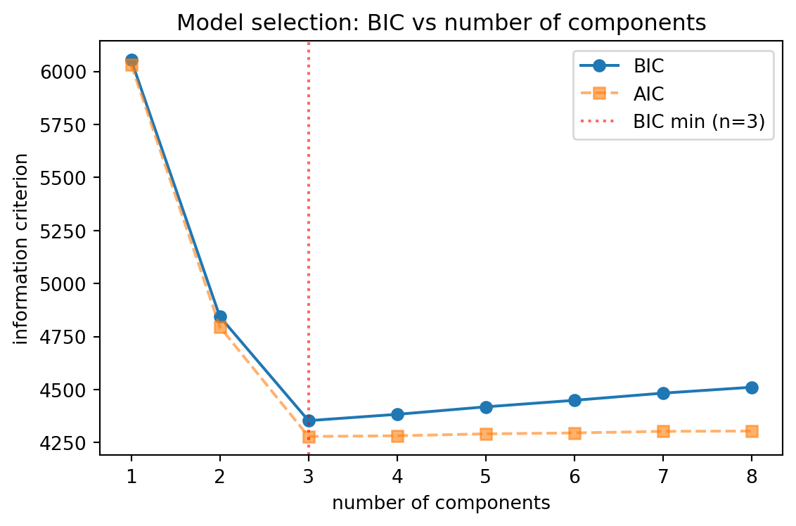
The cell below runs the recipe over the number of components for the same synthetic data, which was generated from three Gaussians. BIC reaches its minimum at three components, recovering the true generating structure, while AIC’s lighter penalty leaves it flatter on the high side. Lower is better, so the minimum of the BIC curve marks the selected model.
Code
import pandas as pdrecords = []for n inrange(1, 9): g = GaussianMixture(n_components=n, covariance_type="full", n_init=5, random_state=0).fit(X) records.append({"n_components": n, "BIC": g.bic(X), "AIC": g.aic(X)})table = pd.DataFrame(records)best_n =int(table.loc[table["BIC"].idxmin(), "n_components"])print(table.to_string(index=False))print("BIC-selected number of components:", best_n)fig, ax = plt.subplots(figsize=(6, 4))ax.plot(table["n_components"], table["BIC"], "o-", label="BIC")ax.plot(table["n_components"], table["AIC"], "s--", label="AIC", alpha=0.6)ax.axvline(best_n, color="red", ls=":", alpha=0.6, label=f"BIC min (n={best_n})")ax.set_xlabel("number of components")ax.set_ylabel("information criterion")ax.set_title("Model selection: BIC vs number of components")ax.legend()plt.tight_layout()plt.show()
Two cautions temper the mechanical use of BIC. First, it answers a statistical question, not a substantive one. The BIC optimal number of components is the one that best explains the density of the data, which need not coincide with the number of semantically meaningful clusters a domain expert would name. A single skewed or heavy tailed group can demand two Gaussians to fit, inflating \(K\) beyond the intuitive cluster count. Second, BIC’s consistency guarantee assumes the data really were generated by a finite Gaussian mixture. Real data rarely are, so treat BIC as a well calibrated heuristic for comparing candidates rather than as ground truth. When the BIC curve is flat near its minimum, prefer the simpler model, and corroborate the choice with held out likelihood, stability across restarts, and visual inspection where dimensionality permits.
134.7 7. Practical Summary
A Gaussian mixture model is a latent variable model whose hidden component indicator, once marginalized, yields a flexible mixture density and, once conditioned on, yields the soft responsibilities that EM iterates over. The log likelihood it maximizes is nonconvex and unbounded, which mandates multiple restarts, covariance regularization, and log domain computation through Cholesky factors. The covariance type, ranging from spherical through diagonal and tied to full, governs the bias variance tradeoff and the parameter budget, while the number of components governs resolution. Both structural choices are resolved by minimizing BIC over a grid, tempered by the understanding that BIC optimizes density fit rather than interpretability. Handled with these safeguards, the GMM remains one of the most useful and well understood tools for probabilistic clustering and density estimation.
134.8 References
Bishop, C. M. Pattern Recognition and Machine Learning, Chapter 9: Mixture Models and EM. Springer, 2006. https://www.microsoft.com/en-us/research/publication/pattern-recognition-machine-learning/
Dempster, A. P., Laird, N. M., and Rubin, D. B. “Maximum Likelihood from Incomplete Data via the EM Algorithm.” Journal of the Royal Statistical Society, Series B, 39(1), 1977. https://www.jstor.org/stable/2984875
Schwarz, G. “Estimating the Dimension of a Model.” The Annals of Statistics, 6(2), 1978. https://www.jstor.org/stable/2958889
McLachlan, G. J., and Peel, D. Finite Mixture Models. Wiley, 2000. https://onlinelibrary.wiley.com/doi/book/10.1002/0471721182
Pedregosa, F., et al. “Scikit-learn: Machine Learning in Python.” Journal of Machine Learning Research, 12, 2011. Gaussian mixture user guide: https://scikit-learn.org/stable/modules/mixture.html
Murphy, K. P. Probabilistic Machine Learning: An Introduction, Chapter on Mixture Models. MIT Press, 2022. https://probml.github.io/pml-book/book1.html
Source Code
# Gaussian Mixture ModelsGaussian mixture models (GMMs) sit at the crossroads of clustering, density estimation, and probabilistic modeling. Where $k$-means partitions data into disjoint groups by minimizing within cluster distance, a GMM treats the data as samples from a weighted sum of Gaussian densities and infers both the parameters of those densities and the probability that each point belongs to each component. This probabilistic stance buys us soft assignments, a principled likelihood we can optimize and compare, and a generative story that explains how the observed data could have been produced. The price is a nonconvex objective, sensitivity to initialization, and a handful of numerical hazards that a careful practitioner must manage. This chapter develops the model from its latent variable foundations, derives the soft assignment and likelihood machinery, surveys the covariance parameterizations that control model complexity, and closes with model selection by the Bayesian information criterion.## 1. The Generative ModelA Gaussian mixture model assumes that each observation $\mathbf{x} \in \mathbb{R}^d$ is drawn from one of $K$ Gaussian components, but we do not observe which one. The density is a convex combination of component densities:$$p(\mathbf{x} \mid \boldsymbol{\theta}) = \sum_{k=1}^{K} \pi_k \, \mathcal{N}(\mathbf{x} \mid \boldsymbol{\mu}_k, \boldsymbol{\Sigma}_k),$$where $\pi_k$ are the mixing weights satisfying $\pi_k \geq 0$ and $\sum_{k=1}^{K} \pi_k = 1$, and each $\mathcal{N}(\mathbf{x} \mid \boldsymbol{\mu}_k, \boldsymbol{\Sigma}_k)$ is a multivariate Gaussian with mean $\boldsymbol{\mu}_k$ and covariance $\boldsymbol{\Sigma}_k$. The full parameter set is $\boldsymbol{\theta} = \{\pi_k, \boldsymbol{\mu}_k, \boldsymbol{\Sigma}_k\}_{k=1}^{K}$. The multivariate Gaussian density is$$\mathcal{N}(\mathbf{x} \mid \boldsymbol{\mu}, \boldsymbol{\Sigma}) = \frac{1}{(2\pi)^{d/2} |\boldsymbol{\Sigma}|^{1/2}} \exp\!\left( -\tfrac{1}{2} (\mathbf{x} - \boldsymbol{\mu})^\top \boldsymbol{\Sigma}^{-1} (\mathbf{x} - \boldsymbol{\mu}) \right).$$The mixture is far more expressive than a single Gaussian. With enough components a GMM can approximate any smooth density to arbitrary accuracy, which makes it a workhorse for density estimation as well as clustering. The model is also generative in a literal sense: to sample a point, first draw a component index from the categorical distribution over $\{1, \dots, K\}$ with probabilities $\pi_k$, then draw $\mathbf{x}$ from the chosen Gaussian.## 2. The Latent Variable FormulationThe clean way to reason about a GMM is to make the unobserved component identity explicit. Introduce a latent variable $\mathbf{z} \in \{0,1\}^K$ for each observation, a one hot vector in which $z_k = 1$ indicates that the point was generated by component $k$. The latent variable follows a categorical prior:$$p(z_k = 1) = \pi_k, \qquad p(\mathbf{z}) = \prod_{k=1}^{K} \pi_k^{z_k}.$$Conditioned on the component, the observation is Gaussian:$$p(\mathbf{x} \mid z_k = 1) = \mathcal{N}(\mathbf{x} \mid \boldsymbol{\mu}_k, \boldsymbol{\Sigma}_k), \qquad p(\mathbf{x} \mid \mathbf{z}) = \prod_{k=1}^{K} \mathcal{N}(\mathbf{x} \mid \boldsymbol{\mu}_k, \boldsymbol{\Sigma}_k)^{z_k}.$$Marginalizing the latent variable recovers the mixture density of Section 1:$$p(\mathbf{x}) = \sum_{\mathbf{z}} p(\mathbf{z}) \, p(\mathbf{x} \mid \mathbf{z}) = \sum_{k=1}^{K} \pi_k \, \mathcal{N}(\mathbf{x} \mid \boldsymbol{\mu}_k, \boldsymbol{\Sigma}_k).$$This formulation is not just notational hygiene. The latent variable is exactly what the expectation maximization (EM) algorithm reasons about, and the posterior over $\mathbf{z}$ given $\mathbf{x}$ is precisely the soft assignment we develop next.## 3. Soft Assignments and ResponsibilitiesThe quantity that distinguishes a GMM from hard clustering is the posterior probability that a given point belongs to each component. Applying Bayes' rule to the latent variable yields the responsibility:$$\gamma(z_{nk}) \equiv p(z_k = 1 \mid \mathbf{x}_n) = \frac{\pi_k \, \mathcal{N}(\mathbf{x}_n \mid \boldsymbol{\mu}_k, \boldsymbol{\Sigma}_k)}{\sum_{j=1}^{K} \pi_j \, \mathcal{N}(\mathbf{x}_n \mid \boldsymbol{\mu}_j, \boldsymbol{\Sigma}_j)}.$$The numerator is the joint probability that component $k$ generated the point, and the denominator is the marginal evidence $p(\mathbf{x}_n)$ that normalizes across components. By construction $\sum_{k=1}^{K} \gamma(z_{nk}) = 1$, so each point distributes one unit of membership across the components in proportion to how well each explains it.This soft assignment is the substantive difference from $k$-means. A point sitting between two clusters might receive responsibilities of $0.55$ and $0.45$, honestly reflecting ambiguity rather than forcing a binary choice. In fact $k$-means is recoverable as a limiting case: fix every covariance to $\sigma^2 \mathbf{I}$, hold the mixing weights equal, and let $\sigma^2 \to 0$. The responsibilities then collapse onto the nearest centroid, and EM reduces to Lloyd's algorithm. The GMM is therefore a strict generalization that relaxes the equal isotropic variance assumption and the hard assignment.Responsibilities also drive the parameter updates. Define the effective number of points assigned to component $k$ as $N_k = \sum_{n=1}^{N} \gamma(z_{nk})$. The EM maximization step then produces closed form updates that are responsibility weighted versions of the ordinary sample statistics:$$\boldsymbol{\mu}_k = \frac{1}{N_k} \sum_{n=1}^{N} \gamma(z_{nk}) \, \mathbf{x}_n, \qquad\boldsymbol{\Sigma}_k = \frac{1}{N_k} \sum_{n=1}^{N} \gamma(z_{nk}) (\mathbf{x}_n - \boldsymbol{\mu}_k)(\mathbf{x}_n - \boldsymbol{\mu}_k)^\top, \qquad\pi_k = \frac{N_k}{N}.$$Each component's mean is the weighted centroid of the data, its covariance is the weighted scatter, and its mixing weight is the fraction of total responsibility it captured. The expectation step recomputes the responsibilities from the current parameters, and the two steps alternate until convergence.The pseudocode below summarizes a single EM pass. The E-step recomputes responsibilities from the current parameters, and the M-step updates the parameters from those responsibilities, repeating until the log likelihood change falls below a tolerance.```textEM for a GMM (one pass) E-step: for each n, k compute gamma(z_nk) from current params M-step: N_k = sum_n gamma(z_nk) mu_k = (1/N_k) sum_n gamma(z_nk) x_n Sig_k = (1/N_k) sum_n gamma(z_nk) (x_n - mu_k)(x_n - mu_k)^T pi_k = N_k / N repeat until log-likelihood change < tol```The following cell fits a three component GMM with full covariances to synthetic data and draws each fitted component as one and two standard deviation ellipses, illustrating the elliptical, rotated shapes that full covariances capture. The fitted means, covariances, and mixing weights are exactly the responsibility weighted statistics from the M-step above.```{python}import numpy as npimport matplotlib.pyplot as pltfrom matplotlib.patches import Ellipsefrom sklearn.mixture import GaussianMixturerng = np.random.default_rng(0)means_true = [(-3, -3), (0, 4), (4, -1)]covs_true = [ [[1.2, 0.6], [0.6, 0.8]], [[0.7, -0.5], [-0.5, 1.4]], [[1.0, 0.0], [0.0, 0.3]],]X = np.vstack([ rng.multivariate_normal(m, c, size=n)for m, c, n inzip(means_true, covs_true, [200, 200, 200])])gmm = GaussianMixture(n_components=3, covariance_type="full", n_init=5, random_state=0).fit(X)labels = gmm.predict(X)def draw_ellipse(mean, cov, ax, color): vals, vecs = np.linalg.eigh(cov) order = vals.argsort()[::-1] vals, vecs = vals[order], vecs[:, order] angle = np.degrees(np.arctan2(vecs[1, 0], vecs[0, 0]))for nsig in (1, 2): w, h =2* nsig * np.sqrt(vals) ax.add_patch(Ellipse(mean, w, h, angle=angle, fill=False, edgecolor=color, lw=1.5, alpha=0.7))fig, ax = plt.subplots(figsize=(6, 5))colors = ["#1f77b4", "#ff7f0e", "#2ca02c"]for k inrange(3): ax.scatter(X[labels == k, 0], X[labels == k, 1], s=8, color=colors[k], alpha=0.5) draw_ellipse(gmm.means_[k], gmm.covariances_[k], ax, colors[k])ax.set_title("GMM fit: full covariance, 3 components")ax.set_xlabel("x1"); ax.set_ylabel("x2")plt.tight_layout()plt.show()print("converged:", gmm.converged_,"log-likelihood:", round(gmm.score(X) *len(X), 1))```The responsibilities are the soft assignments derived above. Each row sums to one, distributing a single unit of membership across the components in proportion to how well each explains the point.```{python}resp = gmm.predict_proba(X)np.set_printoptions(precision=3, suppress=True)for i in [0, 250, 450]:print(f"point {i}: responsibilities = {resp[i]}, sum = {resp[i].sum():.3f}")```## 4. The LikelihoodGiven $N$ independent observations $\mathbf{X} = \{\mathbf{x}_1, \dots, \mathbf{x}_N\}$, the parameters are fit by maximizing the log likelihood:$$\log p(\mathbf{X} \mid \boldsymbol{\theta}) = \sum_{n=1}^{N} \log \left( \sum_{k=1}^{K} \pi_k \, \mathcal{N}(\mathbf{x}_n \mid \boldsymbol{\mu}_k, \boldsymbol{\Sigma}_k) \right).$$The sum inside the logarithm is the source of every difficulty. Because the log cannot be pushed through the sum, the objective does not factor into per component terms and there is no closed form maximizer. The function is also nonconvex, with multiple local optima and saddle points, so the solution returned by EM depends on initialization. Standard practice is to run EM from several random restarts, or from a $k$-means initialization, and keep the run with the highest likelihood.EM optimizes this objective indirectly. It is guaranteed to increase the log likelihood at every iteration, or leave it unchanged at a stationary point, which follows from the fact that EM maximizes a variational lower bound that touches the true likelihood after each E-step. This monotone ascent property makes EM numerically stable and easy to monitor: track the log likelihood and stop when its increase falls below a tolerance.Two failure modes deserve attention. First, the likelihood is unbounded. If a component's mean coincides with a single data point and its covariance shrinks toward zero, that component's density at the point diverges and the likelihood goes to infinity. These singular solutions are degenerate and must be guarded against, typically by adding a small ridge $\varepsilon \mathbf{I}$ to each covariance (a maximum a posteriori regularization with an inverse Wishart prior) or by resetting any component whose effective count $N_k$ collapses. Second, the likelihood is invariant to relabeling the components. Any permutation of the $K$ labels gives an identical likelihood, so there are $K!$ equivalent optima. This label switching is harmless for clustering and density estimation but matters if one tries to interpret individual component parameters across runs.In practice the per point density should be computed in log space using the log-sum-exp trick to avoid underflow when the exponentials are tiny:```textlog p(x_n) = logsumexp_k ( log pi_k + log N(x_n | mu_k, Sigma_k) )log N(...) computed via a Cholesky factor of Sigma_k: Sigma_k = L L^T quad = || L^{-1} (x - mu) ||^2 logdet = 2 * sum(log diag(L)) log N = -0.5 * (d*log(2pi) + logdet + quad)```The Cholesky factorization serves double duty: it gives a numerically stable route to both the quadratic form and the log determinant, and it fails fast if a covariance has lost positive definiteness, which is a useful early warning of a collapsing component.## 5. Covariance TypesThe covariance parameterization is the main lever for controlling a GMM's flexibility and its parameter count. Richer covariances capture correlated, elongated, or rotated clusters but demand more data and more compute. Four standard choices span the spectrum.### 5.1 Full CovarianceEach component carries its own unrestricted symmetric positive definite matrix $\boldsymbol{\Sigma}_k$. This is the most expressive option: components can be elongated and oriented arbitrarily, capturing any correlation structure among the $d$ dimensions. Each covariance has $d(d+1)/2$ free parameters, so the total scales as $K \cdot d(d+1)/2$, which grows quadratically in dimension. Full covariances are appropriate when clusters are genuinely correlated and data is plentiful relative to $d$.### 5.2 Tied CovarianceAll components share a single covariance matrix $\boldsymbol{\Sigma}$, so they differ only in location. This encodes the assumption that every cluster has the same shape and orientation, an assumption identical to the one underlying linear discriminant analysis. It costs only $d(d+1)/2$ covariance parameters in total regardless of $K$, which is a strong regularizer when components are few or data is scarce.### 5.3 Diagonal CovarianceEach component has a diagonal covariance, $\boldsymbol{\Sigma}_k = \mathrm{diag}(\sigma_{k1}^2, \dots, \sigma_{kd}^2)$. This assumes the features are uncorrelated within each component, so the Gaussians are axis aligned ellipsoids that can stretch differently along each dimension but cannot rotate. The cost is only $d$ parameters per component. Diagonal covariances are the default in high dimensional settings such as speaker recognition, where full covariances would be statistically and computationally prohibitive.### 5.4 Spherical CovarianceThe most constrained option sets $\boldsymbol{\Sigma}_k = \sigma_k^2 \mathbf{I}$, a single scalar variance per component. Each cluster is a sphere that can vary in size but not in shape or orientation. This costs one parameter per component and is the assumption that, with equal variances and weights, reduces the GMM to $k$-means.The progression from spherical to diagonal to tied to full trades bias for variance. A useful summary of the parameter budget, where $K$ is the number of components and $d$ the dimension:```textspherical : K covariance parametersdiagonal : K * dtied : d(d+1)/2full : K * d(d+1)/2```Choosing among these is itself a model selection question. The right covariance type is not a fixed preference but a hypothesis to be tested against held out likelihood or an information criterion, which brings us to the final section.## 6. Model Selection with BICA GMM has two structural choices that the likelihood alone cannot make: the number of components $K$ and the covariance type. Maximized likelihood always increases as we add components or relax the covariance, because a more flexible model can fit the training data more closely, so likelihood by itself overfits. We need a criterion that penalizes complexity.The Bayesian information criterion (BIC) supplies exactly such a penalty. For a model with $p$ free parameters fit to $N$ observations with maximized log likelihood $\hat{\mathcal{L}}$, it is defined as$$\mathrm{BIC} = -2 \hat{\mathcal{L}} + p \log N.$$Lower BIC is better. The first term rewards fit and the second penalizes parameter count, with a penalty that grows logarithmically in the sample size. BIC arises as a large sample approximation to the log marginal likelihood (the model evidence) under a Bayesian treatment, dropping terms that vanish as $N \to \infty$. Because the penalty scales with $\log N$, BIC favors more parsimonious models than the Akaike information criterion, whose penalty is the constant $2p$. As a consequence BIC is consistent: if the data truly come from a finite mixture, BIC selects the correct number of components with probability approaching one as $N$ grows, whereas AIC tends to overestimate $K$.The parameter count $p$ must include every free parameter. For a $K$ component GMM in $d$ dimensions there are $K - 1$ free mixing weights (one is fixed by the constraint that they sum to one), $K \cdot d$ mean parameters, and a covariance count that depends on the type chosen in Section 5. For full covariances, for example,$$p = \underbrace{(K-1)}_{\text{weights}} + \underbrace{K d}_{\text{means}} + \underbrace{K \frac{d(d+1)}{2}}_{\text{covariances}}.$$The practical recipe is a grid search. Fit GMMs across a range of $K$ and across the candidate covariance types, compute BIC for each, and select the configuration with the minimum. Because EM finds local optima, each configuration should be fit from several restarts and scored by its best likelihood.```textbest = Nonefor cov_type in [spherical, diagonal, tied, full]: for K in 1..K_max: fit GMM (several restarts, keep best log-likelihood) bic = -2 * loglik + p(K, d, cov_type) * log(N) if best is None or bic < best.bic: best = (K, cov_type, bic)return best```The cell below runs the recipe over the number of components for the same synthetic data, which was generated from three Gaussians. BIC reaches its minimum at three components, recovering the true generating structure, while AIC's lighter penalty leaves it flatter on the high side. Lower is better, so the minimum of the BIC curve marks the selected model.```{python}import pandas as pdrecords = []for n inrange(1, 9): g = GaussianMixture(n_components=n, covariance_type="full", n_init=5, random_state=0).fit(X) records.append({"n_components": n, "BIC": g.bic(X), "AIC": g.aic(X)})table = pd.DataFrame(records)best_n =int(table.loc[table["BIC"].idxmin(), "n_components"])print(table.to_string(index=False))print("BIC-selected number of components:", best_n)fig, ax = plt.subplots(figsize=(6, 4))ax.plot(table["n_components"], table["BIC"], "o-", label="BIC")ax.plot(table["n_components"], table["AIC"], "s--", label="AIC", alpha=0.6)ax.axvline(best_n, color="red", ls=":", alpha=0.6, label=f"BIC min (n={best_n})")ax.set_xlabel("number of components")ax.set_ylabel("information criterion")ax.set_title("Model selection: BIC vs number of components")ax.legend()plt.tight_layout()plt.show()```Two cautions temper the mechanical use of BIC. First, it answers a statistical question, not a substantive one. The BIC optimal number of components is the one that best explains the density of the data, which need not coincide with the number of semantically meaningful clusters a domain expert would name. A single skewed or heavy tailed group can demand two Gaussians to fit, inflating $K$ beyond the intuitive cluster count. Second, BIC's consistency guarantee assumes the data really were generated by a finite Gaussian mixture. Real data rarely are, so treat BIC as a well calibrated heuristic for comparing candidates rather than as ground truth. When the BIC curve is flat near its minimum, prefer the simpler model, and corroborate the choice with held out likelihood, stability across restarts, and visual inspection where dimensionality permits.## 7. Practical SummaryA Gaussian mixture model is a latent variable model whose hidden component indicator, once marginalized, yields a flexible mixture density and, once conditioned on, yields the soft responsibilities that EM iterates over. The log likelihood it maximizes is nonconvex and unbounded, which mandates multiple restarts, covariance regularization, and log domain computation through Cholesky factors. The covariance type, ranging from spherical through diagonal and tied to full, governs the bias variance tradeoff and the parameter budget, while the number of components governs resolution. Both structural choices are resolved by minimizing BIC over a grid, tempered by the understanding that BIC optimizes density fit rather than interpretability. Handled with these safeguards, the GMM remains one of the most useful and well understood tools for probabilistic clustering and density estimation.## References1. Bishop, C. M. *Pattern Recognition and Machine Learning*, Chapter 9: Mixture Models and EM. Springer, 2006. https://www.microsoft.com/en-us/research/publication/pattern-recognition-machine-learning/2. Dempster, A. P., Laird, N. M., and Rubin, D. B. "Maximum Likelihood from Incomplete Data via the EM Algorithm." *Journal of the Royal Statistical Society, Series B*, 39(1), 1977. https://www.jstor.org/stable/29848753. Schwarz, G. "Estimating the Dimension of a Model." *The Annals of Statistics*, 6(2), 1978. https://www.jstor.org/stable/29588894. McLachlan, G. J., and Peel, D. *Finite Mixture Models*. Wiley, 2000. https://onlinelibrary.wiley.com/doi/book/10.1002/04717211825. Pedregosa, F., et al. "Scikit-learn: Machine Learning in Python." *Journal of Machine Learning Research*, 12, 2011. Gaussian mixture user guide: https://scikit-learn.org/stable/modules/mixture.html6. Murphy, K. P. *Probabilistic Machine Learning: An Introduction*, Chapter on Mixture Models. MIT Press, 2022. https://probml.github.io/pml-book/book1.html