Probability distributions are the vocabulary of machine learning. Every likelihood function, every loss derived from maximum likelihood, every generative model, and every Bayesian prior is built from a small set of canonical distributions. Mastering this vocabulary lets you read model specifications fluently, choose appropriate likelihoods for new data types, and reason about uncertainty in a principled way. This chapter surveys the distributions that appear most often in practice. For each one we give the definition, its parameters, the mean and variance, and the role it plays in machine learning. We close with a discussion of conjugacy, the algebraic property that makes Bayesian updating tractable.
33.1 1. Discrete Distributions over Counts and Categories
Discrete distributions place probability mass on a countable set of outcomes. They model binary events, counts, and categorical labels, which together cover a large fraction of supervised learning targets.
33.1.1 1.1 Bernoulli
The Bernoulli distribution describes a single binary trial with two outcomes, success and failure, encoded as \(1\) and \(0\). It has a single parameter \(p \in [0, 1]\), the probability of success. For a random variable \(X\) taking values in \(\{0, 1\}\),
The mean is \(\mathbb{E}[X] = p\) and the variance is \(\operatorname{Var}(X) = p(1 - p)\). The variance is maximized at \(p = 0.5\), where the outcome is most uncertain, and vanishes at the deterministic endpoints \(p = 0\) and \(p = 1\).
In machine learning the Bernoulli is the likelihood behind binary classification. Logistic regression and any binary classifier with a sigmoid output head model the label as Bernoulli with \(p = \sigma(\mathbf{w}^\top \mathbf{x})\), and the negative log likelihood of this model is exactly the binary cross entropy loss. The Bernoulli also appears as the noise model in binary latent variable methods such as restricted Boltzmann machines, and as the per pixel likelihood for binarized images in early variational autoencoders.
33.1.2 1.2 Binomial
The binomial distribution counts the number of successes in \(n\) independent Bernoulli trials that share the same success probability \(p\). It has two parameters, the number of trials \(n \in \{1, 2, \dots\}\) and the success probability \(p \in [0, 1]\). For \(X \in \{0, 1, \dots, n\}\),
The binomial coefficient \(\binom{n}{k}\) counts the number of distinct orderings of \(k\) successes among \(n\) trials. The mean is \(\mathbb{E}[X] = np\) and the variance is \(\operatorname{Var}(X) = np(1 - p)\), both of which follow from summing \(n\) independent Bernoulli variables. A Bernoulli is simply a binomial with \(n = 1\).
In machine learning the binomial models aggregated binary outcomes such as the number of clicks among a fixed number of impressions, or the number of correct predictions on a held out test set of fixed size. This second use is the foundation for confidence intervals on classifier accuracy. The binomial likelihood also underlies A/B testing and the evaluation of pass rates for code generation benchmarks, where each problem is a trial and we count how many were solved.
33.1.3 1.3 Categorical and Multinomial
The categorical distribution generalizes the Bernoulli from two outcomes to \(K\) outcomes. A single trial lands in exactly one of \(K\) categories, with probabilities \(\boldsymbol{\pi} = (\pi_1, \dots, \pi_K)\) satisfying \(\pi_k \ge 0\) and \(\sum_k \pi_k = 1\). If we encode the outcome as a one hot vector \(\mathbf{x}\) with \(x_k = 1\) for the chosen category,
For the indicator of category \(k\), the mean is \(\pi_k\) and the variance is \(\pi_k(1 - \pi_k)\), mirroring the Bernoulli component by component.
The multinomial distribution extends the categorical to \(n\) independent trials, counting how many land in each category. With counts \(\mathbf{n} = (n_1, \dots, n_K)\) where \(\sum_k n_k = n\),
The mean of count \(n_k\) is \(n \pi_k\) and its variance is \(n \pi_k (1 - \pi_k)\), while distinct counts have negative covariance \(\operatorname{Cov}(n_i, n_j) = -n \pi_i \pi_j\) because the total is fixed.
The categorical distribution is the workhorse of multiclass classification. Any neural network that ends in a softmax layer treats the label as categorical with \(\boldsymbol{\pi} = \operatorname{softmax}(\mathbf{z})\), and the cross entropy loss is the negative log likelihood of that categorical model. Language models predict the next token as a categorical distribution over the vocabulary, so every step of autoregressive text generation is a categorical draw. The multinomial appears in bag of words text models such as multinomial naive Bayes and latent Dirichlet allocation, where a document is a vector of word counts.
33.2 2. Continuous Distributions on the Real Line
Continuous distributions assign probability density rather than mass, and they model measurements, errors, and latent quantities that vary smoothly.
33.2.1 2.1 Gaussian, Univariate
The Gaussian or normal distribution is the most important continuous distribution in statistics and machine learning. In one dimension it has two parameters, the mean \(\mu \in \mathbb{R}\) and the variance \(\sigma^2 > 0\). Its density is
The mean is \(\mathbb{E}[X] = \mu\) and the variance is \(\operatorname{Var}(X) = \sigma^2\), so the two parameters are exactly the first two moments. The density is symmetric and bell shaped, with roughly 68 percent of mass within one standard deviation of the mean and 95 percent within two.
The Gaussian owes its ubiquity to the central limit theorem, which states that sums of many independent finite variance contributions converge to a Gaussian regardless of the underlying distribution. This makes it the default model for additive noise. In machine learning, minimizing squared error is equivalent to maximum likelihood under a Gaussian noise model, so linear regression and most regression networks carry an implicit Gaussian assumption. Gaussians also serve as priors in ridge regression, where an \(L_2\) penalty corresponds to a zero mean Gaussian prior on weights, and as the base distribution in diffusion models, where data is gradually corrupted toward an isotropic Gaussian and then denoised.
33.2.2 2.2 Gaussian, Multivariate
The multivariate Gaussian generalizes the normal distribution to a vector \(\mathbf{x} \in \mathbb{R}^d\). Its parameters are a mean vector \(\boldsymbol{\mu} \in \mathbb{R}^d\) and a symmetric positive definite covariance matrix \(\boldsymbol{\Sigma} \in \mathbb{R}^{d \times d}\). The density is
The mean is \(\mathbb{E}[\mathbf{x}] = \boldsymbol{\mu}\) and the covariance is \(\operatorname{Cov}(\mathbf{x}) = \boldsymbol{\Sigma}\). The diagonal entries of \(\boldsymbol{\Sigma}\) give the variance of each coordinate, and the off diagonal entries capture linear dependence between coordinates. The quadratic form in the exponent, \((\mathbf{x} - \boldsymbol{\mu})^\top \boldsymbol{\Sigma}^{-1} (\mathbf{x} - \boldsymbol{\mu})\), is the squared Mahalanobis distance, which measures distance in units that account for the spread and correlation of the data.
Multivariate Gaussians are central to many methods. Gaussian mixture models represent complex densities as weighted sums of Gaussians and are fit with the expectation maximization algorithm. Gaussian processes place a multivariate Gaussian prior over function values and yield closed form posterior uncertainty. Linear discriminant analysis assumes class conditional multivariate Gaussians with shared covariance. Variational autoencoders use a multivariate Gaussian, usually with diagonal covariance, as both the approximate posterior over latent codes and the prior.
33.2.3 2.3 Poisson
The Poisson distribution models the number of events occurring in a fixed interval of time or space when events happen independently at a constant average rate. It has a single parameter, the rate \(\lambda > 0\). For \(X \in \{0, 1, 2, \dots\}\),
A striking property is that the mean and variance are equal, \(\mathbb{E}[X] = \operatorname{Var}(X) = \lambda\). The Poisson arises as the limit of a binomial when \(n \to \infty\) and \(p \to 0\) with \(np = \lambda\) held fixed, which is why it describes rare events over many opportunities.
In machine learning the Poisson is the likelihood for count regression. Poisson regression, a generalized linear model with a log link, predicts counts such as the number of website visits, insurance claims, or photon arrivals. When the equal mean variance constraint is too rigid, practitioners turn to the negative binomial as an overdispersed alternative. The Poisson also models event streams in point process methods and serves as the emission distribution in some sequence models for counts.
33.2.4 2.4 Exponential
The exponential distribution models the waiting time until the next event in a Poisson process. It has a single rate parameter \(\lambda > 0\) and is supported on the nonnegative reals. Its density is
The mean is \(\mathbb{E}[X] = 1/\lambda\) and the variance is \(\operatorname{Var}(X) = 1/\lambda^2\). The exponential is the unique continuous distribution that is memoryless, meaning \(P(X > s + t \mid X > s) = P(X > t)\). The time already waited gives no information about the time remaining.
In machine learning the exponential is the basic likelihood for survival analysis and time to event modeling, where we predict durations such as time until customer churn, equipment failure, or recovery. It appears in hazard rate models and in the simulation of Poisson processes. As a member of the exponential family it also enters maximum entropy derivations, where it is the maximum entropy distribution on the positive reals given a fixed mean.
33.2.5 2.5 Uniform
The continuous uniform distribution places equal density over a bounded interval \([a, b]\) with \(a < b\). Its parameters are the two endpoints \(a\) and \(b\). The density is
\[
p(x \mid a, b) = \frac{1}{b - a}, \quad a \le x \le b,
\]
and zero outside the interval. The mean is \(\mathbb{E}[X] = (a + b)/2\) and the variance is \(\operatorname{Var}(X) = (b - a)^2 / 12\).
The uniform distribution is the natural model of complete ignorance over a bounded range and the default noninformative prior on a finite interval. In practice its most important machine learning role is as the source of randomness for sampling. Inverse transform sampling converts uniform draws into draws from any target distribution through the inverse cumulative distribution function, and pseudorandom number generators produce uniform variates as their primitive output. Uniform initialization schemes set neural network weights from a bounded uniform range, and uniform noise is used in dequantization and in certain exploration strategies for reinforcement learning.
33.3 3. Distributions over Probabilities
The final family models quantities that are themselves probabilities. Because their support is the unit interval or the probability simplex, they are the natural priors for the parameters of Bernoulli, categorical, and multinomial likelihoods.
33.3.1 3.1 Beta
The Beta distribution is a continuous distribution on the unit interval \([0, 1]\), which makes it ideal for modeling an unknown probability. It has two positive shape parameters \(\alpha > 0\) and \(\beta > 0\). Its density is
where \(B(\alpha, \beta) = \Gamma(\alpha)\Gamma(\beta) / \Gamma(\alpha + \beta)\) is the Beta function that normalizes the density. The mean is \(\mathbb{E}[\theta] = \alpha / (\alpha + \beta)\) and the variance is
The shape parameters can be read as pseudocounts of prior successes and failures. When \(\alpha = \beta = 1\) the Beta reduces to the uniform distribution, while large values of \(\alpha\) and \(\beta\) concentrate the density and express confidence.
The Beta is the standard prior for a Bernoulli or binomial probability. It is the engine behind Thompson sampling for Bernoulli bandits, where each arm carries a Beta belief that is updated as rewards arrive. It also models calibration probabilities and click through rates, and it serves as the marginal of a Dirichlet over any single category.
33.3.2 3.2 Dirichlet
The Dirichlet distribution generalizes the Beta from the unit interval to the probability simplex, the set of vectors \(\boldsymbol{\theta} = (\theta_1, \dots, \theta_K)\) with \(\theta_k \ge 0\) and \(\sum_k \theta_k = 1\). It is parameterized by a concentration vector \(\boldsymbol{\alpha} = (\alpha_1, \dots, \alpha_K)\) with each \(\alpha_k > 0\). The density is
where \(B(\boldsymbol{\alpha}) = \prod_k \Gamma(\alpha_k) / \Gamma(\sum_k \alpha_k)\) is the multivariate Beta function. Writing \(\alpha_0 = \sum_k \alpha_k\), the mean of component \(k\) is \(\mathbb{E}[\theta_k] = \alpha_k / \alpha_0\) and its variance is
The total concentration \(\alpha_0\) controls how tightly the draws cluster around the mean: small values produce sparse, peaked vectors near the corners of the simplex, while large values produce nearly uniform vectors.
The Dirichlet is the standard prior over categorical and multinomial parameters. It is the cornerstone of latent Dirichlet allocation, where it generates both the topic mixture of each document and the word distribution of each topic. It also serves as the prior in Bayesian mixture models and as a smoothing mechanism in language modeling, where adding \(\boldsymbol{\alpha}\) to observed counts is equivalent to Dirichlet smoothing.
33.4 4. Derivations of Means, Variances, and Normalizers
The moments quoted above are not arbitrary. Each follows from the definition of the distribution by a short calculation, and working through these derivations builds the fluency needed to handle distributions that are not on any reference card. This section derives the mean and variance of the five core distributions, the normalizing constant of the Gaussian, the multivariate Gaussian density, and the conjugacy relationships that the next section relies on.
33.4.1 4.1 Bernoulli
For \(X \sim \operatorname{Bernoulli}(p)\) the support is \(\{0, 1\}\), so the mean is a two term sum,
\[
\mathbb{E}[X] = 0 \cdot (1 - p) + 1 \cdot p = p.
\]
Because \(X \in \{0, 1\}\) we have \(X^2 = X\), hence \(\mathbb{E}[X^2] = \mathbb{E}[X] = p\). The variance then follows from the computational form \(\operatorname{Var}(X) = \mathbb{E}[X^2] - (\mathbb{E}[X])^2\),
\[
\operatorname{Var}(X) = p - p^2 = p(1 - p).
\]
33.4.2 4.2 Binomial
Write \(X = \sum_{i=1}^{n} Y_i\) as a sum of \(n\) independent \(\operatorname{Bernoulli}(p)\) variables. Linearity of expectation, which needs no independence, gives the mean directly,
\[
\mathbb{E}[X] = \sum_{i=1}^{n} \mathbb{E}[Y_i] = np.
\]
Variance is additive over independent summands, and here independence is what we use. Since each \(\operatorname{Var}(Y_i) = p(1 - p)\),
This representation as a sum of indicators is the cleanest route to both moments and avoids manipulating binomial coefficients.
33.4.3 4.3 Poisson, full derivation
This is the one derivation we work out end to end, because it exercises the power series tricks that recur throughout probability. Let \(X \sim \operatorname{Poisson}(\lambda)\) with \(P(X = k) = \lambda^k e^{-\lambda}/k!\). We will need the exponential series \(\sum_{k=0}^{\infty} \lambda^k / k! = e^{\lambda}\).
The equality of mean and variance, often summarized as equidispersion, falls straight out of these two sums and is the property that diagnostic checks for Poisson regression test against.
33.4.4 4.4 Gaussian normalization, mean, and variance
We first verify that the Gaussian density integrates to one, which pins down the constant \(1 / \sqrt{2\pi\sigma^2}\). Substituting \(z = (x - \mu)/\sigma\) reduces the task to the standard Gaussian integral,
The remaining integral \(I = \int_{-\infty}^{\infty} e^{-z^2/2}\, dz\) is evaluated by the classic polar coordinate trick of squaring it and passing to two dimensions,
where the factor \(r\) is the Jacobian of the polar change of variables and the radial integral evaluates to one. Hence \(I = \sqrt{2\pi}\), the full integral above is \(\sigma\sqrt{2\pi} = \sqrt{2\pi\sigma^2}\), and dividing by it normalizes the density.
The mean follows by symmetry. With \(z = (x - \mu)/\sigma\) the density is symmetric about \(\mu\), so \(\mathbb{E}[X] = \mu + \sigma\,\mathbb{E}[Z]\) where \(Z\) is standard normal, and \(\mathbb{E}[Z] = 0\) because \(z e^{-z^2/2}\) is odd. For the variance, integration by parts on the standard normal gives \(\mathbb{E}[Z^2] = 1\),
since the boundary term vanishes and the surviving integral is \(\sqrt{2\pi}\). Therefore \(\operatorname{Var}(X) = \sigma^2 \mathbb{E}[Z^2] = \sigma^2\).
33.4.5 4.5 Multivariate Gaussian density
The multivariate density of Section 2.2 can be assembled from the univariate case by a linear change of variables, which also explains where the determinant in the normalizer comes from. Let \(\mathbf{z} \in \mathbb{R}^d\) have independent standard normal coordinates, so its density is the product
Because \(\boldsymbol{\Sigma}\) is symmetric positive definite it has a matrix square root \(\boldsymbol{\Sigma}^{1/2}\). Define \(\mathbf{x} = \boldsymbol{\mu} + \boldsymbol{\Sigma}^{1/2} \mathbf{z}\). The change of variables formula multiplies the density by the inverse absolute Jacobian determinant \(|\det \boldsymbol{\Sigma}^{1/2}|^{-1} = |\boldsymbol{\Sigma}|^{-1/2}\), and inverting the map gives \(\mathbf{z} = \boldsymbol{\Sigma}^{-1/2}(\mathbf{x} - \boldsymbol{\mu})\) so that \(\mathbf{z}^\top \mathbf{z} = (\mathbf{x} - \boldsymbol{\mu})^\top \boldsymbol{\Sigma}^{-1} (\mathbf{x} - \boldsymbol{\mu})\). Substituting both yields
which is exactly the density stated earlier. The construction also makes the moments transparent: \(\mathbb{E}[\mathbf{x}] = \boldsymbol{\mu} + \boldsymbol{\Sigma}^{1/2}\mathbb{E}[\mathbf{z}] = \boldsymbol{\mu}\), and \(\operatorname{Cov}(\mathbf{x}) = \boldsymbol{\Sigma}^{1/2} \operatorname{Cov}(\mathbf{z}) \boldsymbol{\Sigma}^{1/2} = \boldsymbol{\Sigma}^{1/2} \mathbf{I} \boldsymbol{\Sigma}^{1/2} = \boldsymbol{\Sigma}\).
33.4.6 4.6 Exponential
For \(X \sim \operatorname{Exponential}(\lambda)\) the mean is an integration by parts, taking \(u = x\) and \(dv = \lambda e^{-\lambda x} dx\),
The memorylessness quoted in Section 2.4 follows from the survival function \(P(X > t) = e^{-\lambda t}\), since \(P(X > s + t \mid X > s) = e^{-\lambda(s+t)} / e^{-\lambda s} = e^{-\lambda t} = P(X > t)\).
33.4.7 4.7 Conjugacy as a general pattern
The conjugate updates collected in the next section all share one mechanism. When a likelihood belongs to the exponential family it can be written in the form \(p(\mathcal{D} \mid \theta) \propto h(\theta)^{a} g(\theta)^{b}\) for sufficient statistics \(a\) and \(b\) extracted from the data, and a prior of the matching algebraic form \(p(\theta) \propto h(\theta)^{a_0} g(\theta)^{b_0}\) multiplies into a posterior \(p(\theta \mid \mathcal{D}) \propto h(\theta)^{a_0 + a} g(\theta)^{b_0 + b}\) of the same form. The Beta and Bernoulli case in Section 6.2 is the visible instance of this pattern, with \(h(\theta) = \theta\) and \(g(\theta) = 1 - \theta\), and the Dirichlet, Gaussian, and Gamma updates are the same identity applied to richer sufficient statistics.
33.5 5. Numerical Illustration
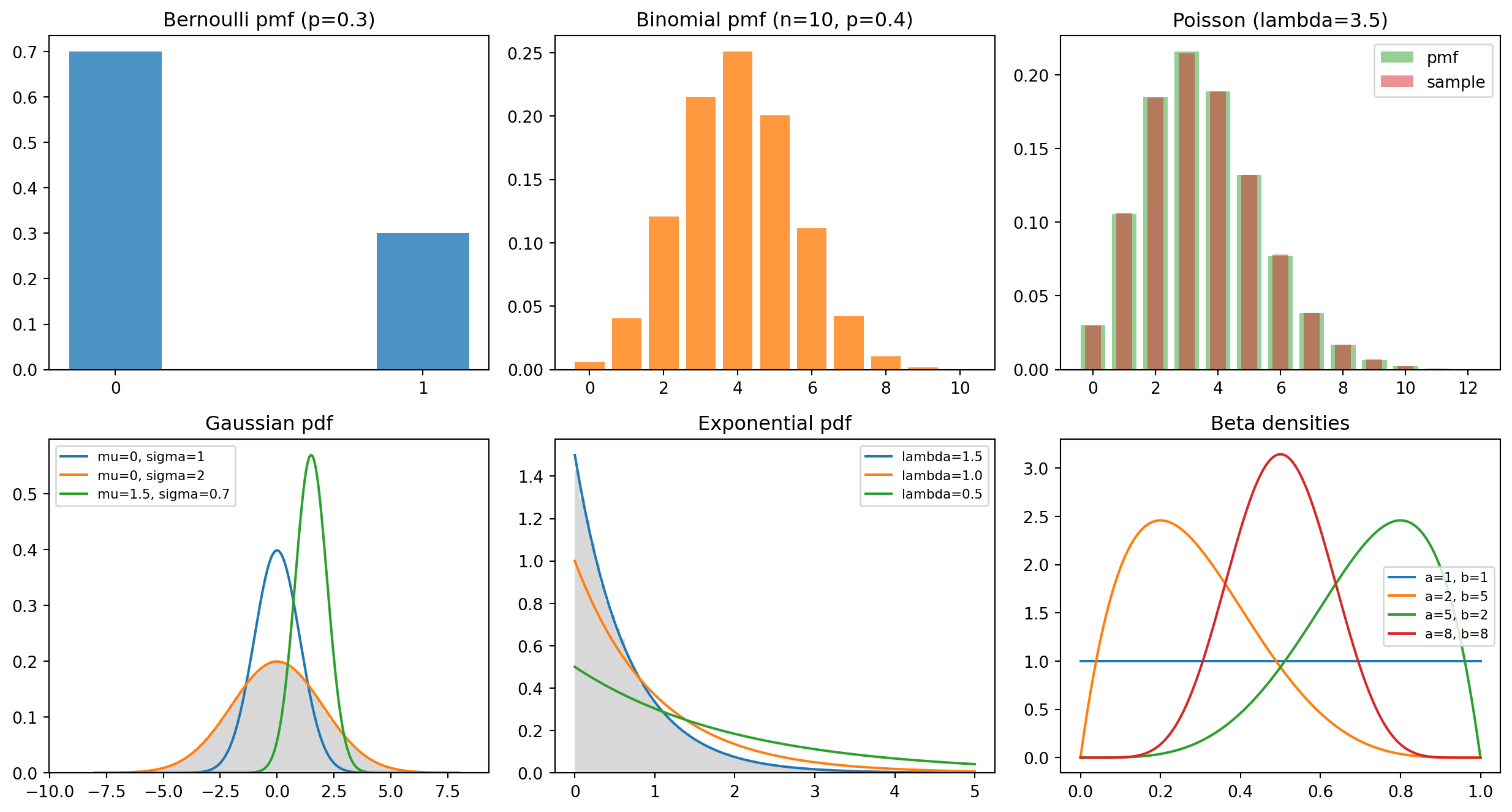
The moments and densities above are easy to check by simulation, and seeing the empirical histograms sit on top of the theoretical curves is the fastest way to build trust in the formulas. The cell below draws large samples from the five core distributions, compares empirical to theoretical means and variances, plots a grid of mass and density functions against sampled histograms, and verifies one Beta to Bernoulli conjugate update numerically. It is fully self contained and runs as written with a fixed seed.
Running the cell prints empirical means and variances that match the theoretical values to within sampling error: the Poisson row shows mean and variance both near \(3.5\), confirming equidispersion, and the exponential row shows mean near \(0.667\) with variance near \(0.444 = 1/\lambda^2\). The figure overlays each theoretical mass or density function on a sampled histogram, and the conjugacy check turns a \(\operatorname{Beta}(2, 2)\) prior into a \(\operatorname{Beta}(33, 11)\) posterior with mean \(0.75\), close to the true success probability of \(0.7\).
// Illustrative: Poisson mean/variance by simulation, no external crates.// Uses a simple LCG and Knuth's algorithm for Poisson sampling.struct Lcg { state:u64}impl Lcg {fn next_f64(&mutself) ->f64{self.state =self.state.wrapping_mul(6364136223846793005).wrapping_add(1); ((self.state >>11) asf64) / ((1u64<<53) asf64)}}fn poisson(rng:&mut Lcg, lambda:f64) ->u64{let l = (-lambda).exp();let (mut k,mut p) = (0u64,1.0f64);loop{ k +=1; p *= rng.next_f64();if p <= l {return k -1;}}}fn main() {letmut rng = Lcg { state:0};let (lambda, n) = (3.5f64,200_000usize);let samples:Vec<f64>= (0..n).map(|_| poisson(&mut rng, lambda) asf64).collect();let mean = samples.iter().sum::<f64>() / n asf64;let var = samples.iter().map(|x| (x - mean).powi(2)).sum::<f64>() / n asf64;println!("Poisson(3.5): mean = {:.4} (thy 3.5), var = {:.4} (thy 3.5)", mean, var);}
33.6 6. Summary Comparison and Conjugacy
33.6.1 6.1 Comparison Table
The table below collects the distributions covered in this chapter, their support, parameters, and moments. It is meant as a quick reference when choosing a likelihood or prior.
Distribution
Support
Parameters
Mean
Variance
Bernoulli
\(\{0, 1\}\)
\(p\)
\(p\)
\(p(1-p)\)
Binomial
\(\{0, \dots, n\}\)
\(n, p\)
\(np\)
\(np(1-p)\)
Categorical
one of \(K\)
\(\boldsymbol{\pi}\)
\(\pi_k\)
\(\pi_k(1-\pi_k)\)
Multinomial
counts summing to \(n\)
\(n, \boldsymbol{\pi}\)
\(n\pi_k\)
\(n\pi_k(1-\pi_k)\)
Gaussian (univariate)
\(\mathbb{R}\)
\(\mu, \sigma^2\)
\(\mu\)
\(\sigma^2\)
Gaussian (multivariate)
\(\mathbb{R}^d\)
\(\boldsymbol{\mu}, \boldsymbol{\Sigma}\)
\(\boldsymbol{\mu}\)
\(\boldsymbol{\Sigma}\)
Poisson
\(\{0, 1, 2, \dots\}\)
\(\lambda\)
\(\lambda\)
\(\lambda\)
Exponential
\([0, \infty)\)
\(\lambda\)
\(1/\lambda\)
\(1/\lambda^2\)
Uniform
\([a, b]\)
\(a, b\)
\((a+b)/2\)
\((b-a)^2/12\)
Beta
\([0, 1]\)
\(\alpha, \beta\)
\(\alpha/(\alpha+\beta)\)
see Section 3.1
Dirichlet
simplex in \(\mathbb{R}^K\)
\(\boldsymbol{\alpha}\)
\(\alpha_k/\alpha_0\)
see Section 3.2
A few patterns are worth noting. The Bernoulli, binomial, categorical, and multinomial form one family of count models that build on each other. The Poisson is the equal mean variance limit of the binomial. The Beta is the one dimensional case of the Dirichlet. Recognizing these relationships reduces a long list to a handful of core ideas.
33.6.2 6.2 Conjugacy
Bayesian inference combines a prior \(p(\theta)\) over a parameter with a likelihood \(p(\mathcal{D} \mid \theta)\) for the data to produce a posterior \(p(\theta \mid \mathcal{D}) \propto p(\mathcal{D} \mid \theta)\, p(\theta)\). In general the posterior has no closed form and must be approximated by sampling or by variational methods. Conjugacy is the happy exception. A prior is conjugate to a likelihood when the posterior belongs to the same family as the prior, differing only in its parameters. Updating then reduces to simple arithmetic on those parameters, which makes the math tractable and the computation cheap.
The clearest example is the Beta and Bernoulli pair. Suppose \(\theta\) has a \(\operatorname{Beta}(\alpha, \beta)\) prior and we observe \(s\) successes and \(f\) failures in independent Bernoulli trials. The posterior is
which is again a Beta, now \(\operatorname{Beta}(\alpha + s, \beta + f)\). We simply add the observed successes and failures to the prior pseudocounts. This is why the parameters of the Beta read so naturally as prior counts.
The same structure generalizes. The Dirichlet is conjugate to the categorical and multinomial: a \(\operatorname{Dirichlet}(\boldsymbol{\alpha})\) prior updated with category counts \(\mathbf{n}\) gives a \(\operatorname{Dirichlet}(\boldsymbol{\alpha} + \mathbf{n})\) posterior. The Gaussian is conjugate to itself for the mean when the variance is known, and the Gamma distribution is the conjugate prior for the precision of a Gaussian and for the rate of a Poisson or exponential likelihood. These conjugate pairs are not coincidental. They all arise because the likelihoods belong to the exponential family, for which a conjugate prior always exists in principle. Conjugacy explains why a small set of distributions appears again and again as priors, and why Bayesian methods built on them, from Thompson sampling to latent Dirichlet allocation, admit efficient closed form updates.
Understanding these distributions and their conjugate relationships gives you a compact toolkit for specifying models. When you face a new prediction target, ask what kind of quantity it is, binary, categorical, a count, a real number, a duration, or a probability, and the appropriate likelihood usually follows directly from the list above. When you want to reason about the parameters of that likelihood in a Bayesian way, the conjugate prior gives you a starting point with interpretable pseudocounts and tractable updates.
33.7 References
Bishop, C. M. Pattern Recognition and Machine Learning. Springer, 2006. ISBN 978-0387310732. https://link.springer.com/book/9780387310732
Murphy, K. P. Probabilistic Machine Learning: An Introduction. MIT Press, 2022. ISBN 978-0262046824. https://probml.github.io/pml-book/book1.html
Murphy, K. P. Machine Learning: A Probabilistic Perspective. MIT Press, 2012. ISBN 978-0262018029. https://mitpress.mit.edu/9780262018029/machine-learning/
Gelman, A., Carlin, J. B., Stern, H. S., Dunson, D. B., Vehtari, A., and Rubin, D. B. Bayesian Data Analysis, 3rd edition. Chapman and Hall/CRC, 2013. https://doi.org/10.1201/b16018
Wasserman, L. All of Statistics: A Concise Course in Statistical Inference. Springer, 2004. https://doi.org/10.1007/978-0-387-21736-9
Blei, D. M., Ng, A. Y., and Jordan, M. I. Latent Dirichlet Allocation. Journal of Machine Learning Research, 3:993-1022, 2003. https://www.jmlr.org/papers/v3/blei03a.html
Diaconis, P., and Ylvisaker, D. Conjugate Priors for Exponential Families. The Annals of Statistics, 7(2):269-281, 1979. https://doi.org/10.1214/aos/1176344611
Virtanen, P., et al. SciPy 1.0: Fundamental Algorithms for Scientific Computing in Python. Nature Methods, 17:261-272, 2020. https://doi.org/10.1038/s41592-019-0686-2
Harris, C. R., et al. Array Programming with NumPy. Nature, 585:357-362, 2020. https://doi.org/10.1038/s41586-020-2649-2
Source Code
# Common Probability DistributionsProbability distributions are the vocabulary of machine learning. Every likelihood function, every loss derived from maximum likelihood, every generative model, and every Bayesian prior is built from a small set of canonical distributions. Mastering this vocabulary lets you read model specifications fluently, choose appropriate likelihoods for new data types, and reason about uncertainty in a principled way. This chapter surveys the distributions that appear most often in practice. For each one we give the definition, its parameters, the mean and variance, and the role it plays in machine learning. We close with a discussion of conjugacy, the algebraic property that makes Bayesian updating tractable.## 1. Discrete Distributions over Counts and CategoriesDiscrete distributions place probability mass on a countable set of outcomes. They model binary events, counts, and categorical labels, which together cover a large fraction of supervised learning targets.### 1.1 BernoulliThe Bernoulli distribution describes a single binary trial with two outcomes, success and failure, encoded as $1$ and $0$. It has a single parameter $p \in [0, 1]$, the probability of success. For a random variable $X$ taking values in $\{0, 1\}$,$$P(X = x) = p^x (1 - p)^{1 - x}, \quad x \in \{0, 1\}.$$The mean is $\mathbb{E}[X] = p$ and the variance is $\operatorname{Var}(X) = p(1 - p)$. The variance is maximized at $p = 0.5$, where the outcome is most uncertain, and vanishes at the deterministic endpoints $p = 0$ and $p = 1$.In machine learning the Bernoulli is the likelihood behind binary classification. Logistic regression and any binary classifier with a sigmoid output head model the label as Bernoulli with $p = \sigma(\mathbf{w}^\top \mathbf{x})$, and the negative log likelihood of this model is exactly the binary cross entropy loss. The Bernoulli also appears as the noise model in binary latent variable methods such as restricted Boltzmann machines, and as the per pixel likelihood for binarized images in early variational autoencoders.### 1.2 BinomialThe binomial distribution counts the number of successes in $n$ independent Bernoulli trials that share the same success probability $p$. It has two parameters, the number of trials $n \in \{1, 2, \dots\}$ and the success probability $p \in [0, 1]$. For $X \in \{0, 1, \dots, n\}$,$$P(X = k) = \binom{n}{k} p^k (1 - p)^{n - k}.$$The binomial coefficient $\binom{n}{k}$ counts the number of distinct orderings of $k$ successes among $n$ trials. The mean is $\mathbb{E}[X] = np$ and the variance is $\operatorname{Var}(X) = np(1 - p)$, both of which follow from summing $n$ independent Bernoulli variables. A Bernoulli is simply a binomial with $n = 1$.In machine learning the binomial models aggregated binary outcomes such as the number of clicks among a fixed number of impressions, or the number of correct predictions on a held out test set of fixed size. This second use is the foundation for confidence intervals on classifier accuracy. The binomial likelihood also underlies A/B testing and the evaluation of pass rates for code generation benchmarks, where each problem is a trial and we count how many were solved.### 1.3 Categorical and MultinomialThe categorical distribution generalizes the Bernoulli from two outcomes to $K$ outcomes. A single trial lands in exactly one of $K$ categories, with probabilities $\boldsymbol{\pi} = (\pi_1, \dots, \pi_K)$ satisfying $\pi_k \ge 0$ and $\sum_k \pi_k = 1$. If we encode the outcome as a one hot vector $\mathbf{x}$ with $x_k = 1$ for the chosen category,$$P(\mathbf{x} \mid \boldsymbol{\pi}) = \prod_{k=1}^{K} \pi_k^{x_k}.$$For the indicator of category $k$, the mean is $\pi_k$ and the variance is $\pi_k(1 - \pi_k)$, mirroring the Bernoulli component by component.The multinomial distribution extends the categorical to $n$ independent trials, counting how many land in each category. With counts $\mathbf{n} = (n_1, \dots, n_K)$ where $\sum_k n_k = n$,$$P(\mathbf{n} \mid \boldsymbol{\pi}, n) = \frac{n!}{n_1! \cdots n_K!} \prod_{k=1}^{K} \pi_k^{n_k}.$$The mean of count $n_k$ is $n \pi_k$ and its variance is $n \pi_k (1 - \pi_k)$, while distinct counts have negative covariance $\operatorname{Cov}(n_i, n_j) = -n \pi_i \pi_j$ because the total is fixed.The categorical distribution is the workhorse of multiclass classification. Any neural network that ends in a softmax layer treats the label as categorical with $\boldsymbol{\pi} = \operatorname{softmax}(\mathbf{z})$, and the cross entropy loss is the negative log likelihood of that categorical model. Language models predict the next token as a categorical distribution over the vocabulary, so every step of autoregressive text generation is a categorical draw. The multinomial appears in bag of words text models such as multinomial naive Bayes and latent Dirichlet allocation, where a document is a vector of word counts.## 2. Continuous Distributions on the Real LineContinuous distributions assign probability density rather than mass, and they model measurements, errors, and latent quantities that vary smoothly.### 2.1 Gaussian, UnivariateThe Gaussian or normal distribution is the most important continuous distribution in statistics and machine learning. In one dimension it has two parameters, the mean $\mu \in \mathbb{R}$ and the variance $\sigma^2 > 0$. Its density is$$p(x \mid \mu, \sigma^2) = \frac{1}{\sqrt{2 \pi \sigma^2}} \exp\!\left( -\frac{(x - \mu)^2}{2 \sigma^2} \right).$$The mean is $\mathbb{E}[X] = \mu$ and the variance is $\operatorname{Var}(X) = \sigma^2$, so the two parameters are exactly the first two moments. The density is symmetric and bell shaped, with roughly 68 percent of mass within one standard deviation of the mean and 95 percent within two.The Gaussian owes its ubiquity to the central limit theorem, which states that sums of many independent finite variance contributions converge to a Gaussian regardless of the underlying distribution. This makes it the default model for additive noise. In machine learning, minimizing squared error is equivalent to maximum likelihood under a Gaussian noise model, so linear regression and most regression networks carry an implicit Gaussian assumption. Gaussians also serve as priors in ridge regression, where an $L_2$ penalty corresponds to a zero mean Gaussian prior on weights, and as the base distribution in diffusion models, where data is gradually corrupted toward an isotropic Gaussian and then denoised.### 2.2 Gaussian, MultivariateThe multivariate Gaussian generalizes the normal distribution to a vector $\mathbf{x} \in \mathbb{R}^d$. Its parameters are a mean vector $\boldsymbol{\mu} \in \mathbb{R}^d$ and a symmetric positive definite covariance matrix $\boldsymbol{\Sigma} \in \mathbb{R}^{d \times d}$. The density is$$p(\mathbf{x} \mid \boldsymbol{\mu}, \boldsymbol{\Sigma}) = \frac{1}{(2\pi)^{d/2} |\boldsymbol{\Sigma}|^{1/2}} \exp\!\left( -\tfrac{1}{2} (\mathbf{x} - \boldsymbol{\mu})^\top \boldsymbol{\Sigma}^{-1} (\mathbf{x} - \boldsymbol{\mu}) \right).$$The mean is $\mathbb{E}[\mathbf{x}] = \boldsymbol{\mu}$ and the covariance is $\operatorname{Cov}(\mathbf{x}) = \boldsymbol{\Sigma}$. The diagonal entries of $\boldsymbol{\Sigma}$ give the variance of each coordinate, and the off diagonal entries capture linear dependence between coordinates. The quadratic form in the exponent, $(\mathbf{x} - \boldsymbol{\mu})^\top \boldsymbol{\Sigma}^{-1} (\mathbf{x} - \boldsymbol{\mu})$, is the squared Mahalanobis distance, which measures distance in units that account for the spread and correlation of the data.Multivariate Gaussians are central to many methods. Gaussian mixture models represent complex densities as weighted sums of Gaussians and are fit with the expectation maximization algorithm. Gaussian processes place a multivariate Gaussian prior over function values and yield closed form posterior uncertainty. Linear discriminant analysis assumes class conditional multivariate Gaussians with shared covariance. Variational autoencoders use a multivariate Gaussian, usually with diagonal covariance, as both the approximate posterior over latent codes and the prior.### 2.3 PoissonThe Poisson distribution models the number of events occurring in a fixed interval of time or space when events happen independently at a constant average rate. It has a single parameter, the rate $\lambda > 0$. For $X \in \{0, 1, 2, \dots\}$,$$P(X = k) = \frac{\lambda^k e^{-\lambda}}{k!}.$$A striking property is that the mean and variance are equal, $\mathbb{E}[X] = \operatorname{Var}(X) = \lambda$. The Poisson arises as the limit of a binomial when $n \to \infty$ and $p \to 0$ with $np = \lambda$ held fixed, which is why it describes rare events over many opportunities.In machine learning the Poisson is the likelihood for count regression. Poisson regression, a generalized linear model with a log link, predicts counts such as the number of website visits, insurance claims, or photon arrivals. When the equal mean variance constraint is too rigid, practitioners turn to the negative binomial as an overdispersed alternative. The Poisson also models event streams in point process methods and serves as the emission distribution in some sequence models for counts.### 2.4 ExponentialThe exponential distribution models the waiting time until the next event in a Poisson process. It has a single rate parameter $\lambda > 0$ and is supported on the nonnegative reals. Its density is$$p(x \mid \lambda) = \lambda e^{-\lambda x}, \quad x \ge 0.$$The mean is $\mathbb{E}[X] = 1/\lambda$ and the variance is $\operatorname{Var}(X) = 1/\lambda^2$. The exponential is the unique continuous distribution that is memoryless, meaning $P(X > s + t \mid X > s) = P(X > t)$. The time already waited gives no information about the time remaining.In machine learning the exponential is the basic likelihood for survival analysis and time to event modeling, where we predict durations such as time until customer churn, equipment failure, or recovery. It appears in hazard rate models and in the simulation of Poisson processes. As a member of the exponential family it also enters maximum entropy derivations, where it is the maximum entropy distribution on the positive reals given a fixed mean.### 2.5 UniformThe continuous uniform distribution places equal density over a bounded interval $[a, b]$ with $a < b$. Its parameters are the two endpoints $a$ and $b$. The density is$$p(x \mid a, b) = \frac{1}{b - a}, \quad a \le x \le b,$$and zero outside the interval. The mean is $\mathbb{E}[X] = (a + b)/2$ and the variance is $\operatorname{Var}(X) = (b - a)^2 / 12$.The uniform distribution is the natural model of complete ignorance over a bounded range and the default noninformative prior on a finite interval. In practice its most important machine learning role is as the source of randomness for sampling. Inverse transform sampling converts uniform draws into draws from any target distribution through the inverse cumulative distribution function, and pseudorandom number generators produce uniform variates as their primitive output. Uniform initialization schemes set neural network weights from a bounded uniform range, and uniform noise is used in dequantization and in certain exploration strategies for reinforcement learning.## 3. Distributions over ProbabilitiesThe final family models quantities that are themselves probabilities. Because their support is the unit interval or the probability simplex, they are the natural priors for the parameters of Bernoulli, categorical, and multinomial likelihoods.### 3.1 BetaThe Beta distribution is a continuous distribution on the unit interval $[0, 1]$, which makes it ideal for modeling an unknown probability. It has two positive shape parameters $\alpha > 0$ and $\beta > 0$. Its density is$$p(\theta \mid \alpha, \beta) = \frac{\theta^{\alpha - 1} (1 - \theta)^{\beta - 1}}{B(\alpha, \beta)},$$where $B(\alpha, \beta) = \Gamma(\alpha)\Gamma(\beta) / \Gamma(\alpha + \beta)$ is the Beta function that normalizes the density. The mean is $\mathbb{E}[\theta] = \alpha / (\alpha + \beta)$ and the variance is$$\operatorname{Var}(\theta) = \frac{\alpha \beta}{(\alpha + \beta)^2 (\alpha + \beta + 1)}.$$The shape parameters can be read as pseudocounts of prior successes and failures. When $\alpha = \beta = 1$ the Beta reduces to the uniform distribution, while large values of $\alpha$ and $\beta$ concentrate the density and express confidence.The Beta is the standard prior for a Bernoulli or binomial probability. It is the engine behind Thompson sampling for Bernoulli bandits, where each arm carries a Beta belief that is updated as rewards arrive. It also models calibration probabilities and click through rates, and it serves as the marginal of a Dirichlet over any single category.### 3.2 DirichletThe Dirichlet distribution generalizes the Beta from the unit interval to the probability simplex, the set of vectors $\boldsymbol{\theta} = (\theta_1, \dots, \theta_K)$ with $\theta_k \ge 0$ and $\sum_k \theta_k = 1$. It is parameterized by a concentration vector $\boldsymbol{\alpha} = (\alpha_1, \dots, \alpha_K)$ with each $\alpha_k > 0$. The density is$$p(\boldsymbol{\theta} \mid \boldsymbol{\alpha}) = \frac{1}{B(\boldsymbol{\alpha})} \prod_{k=1}^{K} \theta_k^{\alpha_k - 1},$$where $B(\boldsymbol{\alpha}) = \prod_k \Gamma(\alpha_k) / \Gamma(\sum_k \alpha_k)$ is the multivariate Beta function. Writing $\alpha_0 = \sum_k \alpha_k$, the mean of component $k$ is $\mathbb{E}[\theta_k] = \alpha_k / \alpha_0$ and its variance is$$\operatorname{Var}(\theta_k) = \frac{\alpha_k (\alpha_0 - \alpha_k)}{\alpha_0^2 (\alpha_0 + 1)}.$$The total concentration $\alpha_0$ controls how tightly the draws cluster around the mean: small values produce sparse, peaked vectors near the corners of the simplex, while large values produce nearly uniform vectors.The Dirichlet is the standard prior over categorical and multinomial parameters. It is the cornerstone of latent Dirichlet allocation, where it generates both the topic mixture of each document and the word distribution of each topic. It also serves as the prior in Bayesian mixture models and as a smoothing mechanism in language modeling, where adding $\boldsymbol{\alpha}$ to observed counts is equivalent to Dirichlet smoothing.## 4. Derivations of Means, Variances, and NormalizersThe moments quoted above are not arbitrary. Each follows from the definition of the distribution by a short calculation, and working through these derivations builds the fluency needed to handle distributions that are not on any reference card. This section derives the mean and variance of the five core distributions, the normalizing constant of the Gaussian, the multivariate Gaussian density, and the conjugacy relationships that the next section relies on.### 4.1 BernoulliFor $X \sim \operatorname{Bernoulli}(p)$ the support is $\{0, 1\}$, so the mean is a two term sum,$$\mathbb{E}[X] = 0 \cdot (1 - p) + 1 \cdot p = p.$$Because $X \in \{0, 1\}$ we have $X^2 = X$, hence $\mathbb{E}[X^2] = \mathbb{E}[X] = p$. The variance then follows from the computational form $\operatorname{Var}(X) = \mathbb{E}[X^2] - (\mathbb{E}[X])^2$,$$\operatorname{Var}(X) = p - p^2 = p(1 - p).$$### 4.2 BinomialWrite $X = \sum_{i=1}^{n} Y_i$ as a sum of $n$ independent $\operatorname{Bernoulli}(p)$ variables. Linearity of expectation, which needs no independence, gives the mean directly,$$\mathbb{E}[X] = \sum_{i=1}^{n} \mathbb{E}[Y_i] = np.$$Variance is additive over independent summands, and here independence is what we use. Since each $\operatorname{Var}(Y_i) = p(1 - p)$,$$\operatorname{Var}(X) = \sum_{i=1}^{n} \operatorname{Var}(Y_i) = np(1 - p).$$This representation as a sum of indicators is the cleanest route to both moments and avoids manipulating binomial coefficients.### 4.3 Poisson, full derivationThis is the one derivation we work out end to end, because it exercises the power series tricks that recur throughout probability. Let $X \sim \operatorname{Poisson}(\lambda)$ with $P(X = k) = \lambda^k e^{-\lambda}/k!$. We will need the exponential series $\sum_{k=0}^{\infty} \lambda^k / k! = e^{\lambda}$.First confirm the mass function sums to one,$$\sum_{k=0}^{\infty} \frac{\lambda^k e^{-\lambda}}{k!} = e^{-\lambda} \sum_{k=0}^{\infty} \frac{\lambda^k}{k!} = e^{-\lambda} e^{\lambda} = 1.$$For the mean, the $k = 0$ term vanishes, so we start the sum at $k = 1$ and cancel one factor of $k$ against $k!$,$$\mathbb{E}[X] = \sum_{k=1}^{\infty} k \frac{\lambda^k e^{-\lambda}}{k!} = \lambda e^{-\lambda} \sum_{k=1}^{\infty} \frac{\lambda^{k-1}}{(k-1)!}.$$Substituting $j = k - 1$ turns the remaining sum back into the exponential series,$$\mathbb{E}[X] = \lambda e^{-\lambda} \sum_{j=0}^{\infty} \frac{\lambda^{j}}{j!} = \lambda e^{-\lambda} e^{\lambda} = \lambda.$$For the variance it is easiest to compute the factorial moment $\mathbb{E}[X(X-1)]$, which kills the leading two terms,$$\mathbb{E}[X(X-1)] = \sum_{k=2}^{\infty} k(k-1) \frac{\lambda^k e^{-\lambda}}{k!} = \lambda^2 e^{-\lambda} \sum_{k=2}^{\infty} \frac{\lambda^{k-2}}{(k-2)!} = \lambda^2.$$Since $\mathbb{E}[X(X-1)] = \mathbb{E}[X^2] - \mathbb{E}[X]$, we recover $\mathbb{E}[X^2] = \lambda^2 + \lambda$, and therefore$$\operatorname{Var}(X) = \mathbb{E}[X^2] - (\mathbb{E}[X])^2 = \lambda^2 + \lambda - \lambda^2 = \lambda.$$The equality of mean and variance, often summarized as equidispersion, falls straight out of these two sums and is the property that diagnostic checks for Poisson regression test against.### 4.4 Gaussian normalization, mean, and varianceWe first verify that the Gaussian density integrates to one, which pins down the constant $1 / \sqrt{2\pi\sigma^2}$. Substituting $z = (x - \mu)/\sigma$ reduces the task to the standard Gaussian integral,$$\int_{-\infty}^{\infty} \exp\!\left( -\frac{(x - \mu)^2}{2\sigma^2} \right) dx = \sigma \int_{-\infty}^{\infty} e^{-z^2/2}\, dz.$$The remaining integral $I = \int_{-\infty}^{\infty} e^{-z^2/2}\, dz$ is evaluated by the classic polar coordinate trick of squaring it and passing to two dimensions,$$I^2 = \int_{-\infty}^{\infty}\!\int_{-\infty}^{\infty} e^{-(u^2 + v^2)/2}\, du\, dv = \int_0^{2\pi}\!\int_0^{\infty} e^{-r^2/2}\, r\, dr\, d\theta = 2\pi,$$where the factor $r$ is the Jacobian of the polar change of variables and the radial integral evaluates to one. Hence $I = \sqrt{2\pi}$, the full integral above is $\sigma\sqrt{2\pi} = \sqrt{2\pi\sigma^2}$, and dividing by it normalizes the density.The mean follows by symmetry. With $z = (x - \mu)/\sigma$ the density is symmetric about $\mu$, so $\mathbb{E}[X] = \mu + \sigma\,\mathbb{E}[Z]$ where $Z$ is standard normal, and $\mathbb{E}[Z] = 0$ because $z e^{-z^2/2}$ is odd. For the variance, integration by parts on the standard normal gives $\mathbb{E}[Z^2] = 1$,$$\mathbb{E}[Z^2] = \frac{1}{\sqrt{2\pi}} \int_{-\infty}^{\infty} z \cdot z\, e^{-z^2/2}\, dz = \frac{1}{\sqrt{2\pi}} \left( \left[ -z e^{-z^2/2} \right]_{-\infty}^{\infty} + \int_{-\infty}^{\infty} e^{-z^2/2}\, dz \right) = 1,$$since the boundary term vanishes and the surviving integral is $\sqrt{2\pi}$. Therefore $\operatorname{Var}(X) = \sigma^2 \mathbb{E}[Z^2] = \sigma^2$.### 4.5 Multivariate Gaussian densityThe multivariate density of Section 2.2 can be assembled from the univariate case by a linear change of variables, which also explains where the determinant in the normalizer comes from. Let $\mathbf{z} \in \mathbb{R}^d$ have independent standard normal coordinates, so its density is the product$$p(\mathbf{z}) = \prod_{i=1}^{d} \frac{1}{\sqrt{2\pi}} e^{-z_i^2/2} = \frac{1}{(2\pi)^{d/2}} \exp\!\left( -\tfrac{1}{2} \mathbf{z}^\top \mathbf{z} \right).$$Because $\boldsymbol{\Sigma}$ is symmetric positive definite it has a matrix square root $\boldsymbol{\Sigma}^{1/2}$. Define $\mathbf{x} = \boldsymbol{\mu} + \boldsymbol{\Sigma}^{1/2} \mathbf{z}$. The change of variables formula multiplies the density by the inverse absolute Jacobian determinant $|\det \boldsymbol{\Sigma}^{1/2}|^{-1} = |\boldsymbol{\Sigma}|^{-1/2}$, and inverting the map gives $\mathbf{z} = \boldsymbol{\Sigma}^{-1/2}(\mathbf{x} - \boldsymbol{\mu})$ so that $\mathbf{z}^\top \mathbf{z} = (\mathbf{x} - \boldsymbol{\mu})^\top \boldsymbol{\Sigma}^{-1} (\mathbf{x} - \boldsymbol{\mu})$. Substituting both yields$$p(\mathbf{x}) = \frac{1}{(2\pi)^{d/2} |\boldsymbol{\Sigma}|^{1/2}} \exp\!\left( -\tfrac{1}{2} (\mathbf{x} - \boldsymbol{\mu})^\top \boldsymbol{\Sigma}^{-1} (\mathbf{x} - \boldsymbol{\mu}) \right),$$which is exactly the density stated earlier. The construction also makes the moments transparent: $\mathbb{E}[\mathbf{x}] = \boldsymbol{\mu} + \boldsymbol{\Sigma}^{1/2}\mathbb{E}[\mathbf{z}] = \boldsymbol{\mu}$, and $\operatorname{Cov}(\mathbf{x}) = \boldsymbol{\Sigma}^{1/2} \operatorname{Cov}(\mathbf{z}) \boldsymbol{\Sigma}^{1/2} = \boldsymbol{\Sigma}^{1/2} \mathbf{I} \boldsymbol{\Sigma}^{1/2} = \boldsymbol{\Sigma}$.### 4.6 ExponentialFor $X \sim \operatorname{Exponential}(\lambda)$ the mean is an integration by parts, taking $u = x$ and $dv = \lambda e^{-\lambda x} dx$,$$\mathbb{E}[X] = \int_0^{\infty} x\, \lambda e^{-\lambda x}\, dx = \left[ -x e^{-\lambda x} \right]_0^{\infty} + \int_0^{\infty} e^{-\lambda x}\, dx = 0 + \frac{1}{\lambda} = \frac{1}{\lambda}.$$A second integration by parts gives the second moment $\mathbb{E}[X^2] = 2/\lambda^2$, so the variance is$$\operatorname{Var}(X) = \frac{2}{\lambda^2} - \left( \frac{1}{\lambda} \right)^2 = \frac{1}{\lambda^2}.$$The memorylessness quoted in Section 2.4 follows from the survival function $P(X > t) = e^{-\lambda t}$, since $P(X > s + t \mid X > s) = e^{-\lambda(s+t)} / e^{-\lambda s} = e^{-\lambda t} = P(X > t)$.### 4.7 Conjugacy as a general patternThe conjugate updates collected in the next section all share one mechanism. When a likelihood belongs to the exponential family it can be written in the form $p(\mathcal{D} \mid \theta) \propto h(\theta)^{a} g(\theta)^{b}$ for sufficient statistics $a$ and $b$ extracted from the data, and a prior of the matching algebraic form $p(\theta) \propto h(\theta)^{a_0} g(\theta)^{b_0}$ multiplies into a posterior $p(\theta \mid \mathcal{D}) \propto h(\theta)^{a_0 + a} g(\theta)^{b_0 + b}$ of the same form. The Beta and Bernoulli case in Section 6.2 is the visible instance of this pattern, with $h(\theta) = \theta$ and $g(\theta) = 1 - \theta$, and the Dirichlet, Gaussian, and Gamma updates are the same identity applied to richer sufficient statistics.## 5. Numerical IllustrationThe moments and densities above are easy to check by simulation, and seeing the empirical histograms sit on top of the theoretical curves is the fastest way to build trust in the formulas. The cell below draws large samples from the five core distributions, compares empirical to theoretical means and variances, plots a grid of mass and density functions against sampled histograms, and verifies one Beta to Bernoulli conjugate update numerically. It is fully self contained and runs as written with a fixed seed.::: {.panel-tabset}## Python```{python}import numpy as npimport matplotlib.pyplot as pltfrom scipy import statsrng = np.random.default_rng(0)# 1. Empirical vs theoretical moments for five core distributionsN =200_000specs = {"Bernoulli(p=0.3)": (rng.binomial(1, 0.3, N), 0.3, 0.3*0.7),"Binomial(n=10,p=0.4)": (rng.binomial(10, 0.4, N), 10*0.4, 10*0.4*0.6),"Poisson(l=3.5)": (rng.poisson(3.5, N), 3.5, 3.5),"Gaussian(0,2^2)": (rng.normal(0.0, 2.0, N), 0.0, 4.0),"Exponential(l=1.5)": (rng.exponential(1/1.5, N), 1/1.5, 1/1.5**2),}print(f"{'distribution':22s}{'mean(emp)':>10s}{'mean(thy)':>10s} "f"{'var(emp)':>10s}{'var(thy)':>10s}")for name, (s, m_thy, v_thy) in specs.items():print(f"{name:22s}{s.mean():10.4f}{m_thy:10.4f}{s.var():10.4f}{v_thy:10.4f}")# 2. Grid of pmf / pdf plots with overlaid empirical histogramsfig, axes = plt.subplots(2, 3, figsize=(13, 7))ax = axes[0, 0]k = np.array([0, 1])ax.bar(k, stats.bernoulli.pmf(k, 0.3), width=0.3, color="C0", alpha=0.8)ax.set_title("Bernoulli pmf (p=0.3)"); ax.set_xticks([0, 1])ax = axes[0, 1]k = np.arange(0, 11)ax.bar(k, stats.binom.pmf(k, 10, 0.4), color="C1", alpha=0.8)ax.set_title("Binomial pmf (n=10, p=0.4)")ax = axes[0, 2]k = np.arange(0, 13)ax.bar(k, stats.poisson.pmf(k, 3.5), color="C2", alpha=0.5, label="pmf")s = specs["Poisson(l=3.5)"][0]ax.bar(k, np.bincount(s, minlength=13)[:13] / s.size, color="C3", alpha=0.5, width=0.5, label="sample")ax.set_title("Poisson (lambda=3.5)"); ax.legend()ax = axes[1, 0]xs = np.linspace(-8, 8, 400)for mu, sd, c in [(0, 1, "C0"), (0, 2, "C1"), (1.5, 0.7, "C2")]: ax.plot(xs, stats.norm.pdf(xs, mu, sd), color=c, label=f"mu={mu}, sigma={sd}")ax.hist(specs["Gaussian(0,2^2)"][0], bins=80, density=True, color="grey", alpha=0.3)ax.set_title("Gaussian pdf"); ax.legend(fontsize=8)ax = axes[1, 1]xs = np.linspace(0, 5, 400)for lam, c in [(1.5, "C0"), (1.0, "C1"), (0.5, "C2")]: ax.plot(xs, stats.expon.pdf(xs, scale=1/ lam), color=c, label=f"lambda={lam}")ax.hist(specs["Exponential(l=1.5)"][0], bins=80, density=True,range=(0, 5), color="grey", alpha=0.3)ax.set_title("Exponential pdf"); ax.legend(fontsize=8)ax = axes[1, 2]xs = np.linspace(0, 1, 400)for a, b, c in [(1, 1, "C0"), (2, 5, "C1"), (5, 2, "C2"), (8, 8, "C3")]: ax.plot(xs, stats.beta.pdf(xs, a, b), color=c, label=f"a={a}, b={b}")ax.set_title("Beta densities"); ax.legend(fontsize=8)plt.tight_layout()plt.show()# 3. Beta-Bernoulli conjugacy: prior + counts -> posteriora0, b0, theta_true =2.0, 2.0, 0.7data = rng.binomial(1, theta_true, 40)s_cnt, f_cnt = data.sum(), data.size - data.sum()a_post, b_post = a0 + s_cnt, b0 + f_cntprint(f"\nBeta-Bernoulli: prior Beta({a0},{b0}), observed "f"{s_cnt} successes / {f_cnt} failures")print(f" posterior Beta({a_post},{b_post}), mean = "f"{a_post / (a_post + b_post):.4f}, true theta = {theta_true}")```Running the cell prints empirical means and variances that match the theoretical values to within sampling error: the Poisson row shows mean and variance both near $3.5$, confirming equidispersion, and the exponential row shows mean near $0.667$ with variance near $0.444 = 1/\lambda^2$. The figure overlays each theoretical mass or density function on a sampled histogram, and the conjugacy check turns a $\operatorname{Beta}(2, 2)$ prior into a $\operatorname{Beta}(33, 11)$ posterior with mean $0.75$, close to the true success probability of $0.7$.## Julia```julia# Illustrative: empirical vs theoretical moments in Julia.usingRandom, Statistics, Distributionsrng =MersenneTwister(0)dists =Dict("Bernoulli(0.3)"=>Bernoulli(0.3),"Binomial(10,0.4)"=>Binomial(10, 0.4),"Poisson(3.5)"=>Poisson(3.5),"Normal(0,2)"=>Normal(0.0, 2.0),"Exponential(1.5)"=>Exponential(1/1.5),)N =200_000for (name, d) in dists s =rand(rng, d, N)println(name, ": mean ", round(mean(s), digits=4)," (thy ", round(mean(d), digits=4), ")",", var ", round(var(s), digits=4)," (thy ", round(var(d), digits=4), ")")end# Beta-Bernoulli conjugate updatea0, b0 =2.0, 2.0data =rand(rng, Bernoulli(0.7), 40)s_cnt =sum(data); f_cnt =length(data) - s_cntprintln("posterior Beta(", a0 + s_cnt, ", ", b0 + f_cnt, ")")```## Rust```rust// Illustrative: Poisson mean/variance by simulation, no external crates.// Uses a simple LCG and Knuth's algorithm for Poisson sampling.struct Lcg { state: u64 }impl Lcg { fn next_f64(&mut self) -> f64 { self.state = self.state.wrapping_mul(6364136223846793005).wrapping_add(1); ((self.state >> 11) as f64) / ((1u64 << 53) as f64) }}fn poisson(rng: &mut Lcg, lambda: f64) -> u64 { let l = (-lambda).exp(); let (mut k, mut p) = (0u64, 1.0f64); loop { k += 1; p *= rng.next_f64(); if p <= l { return k - 1; } }}fn main() { let mut rng = Lcg { state: 0 }; let (lambda, n) = (3.5f64, 200_000usize); let samples: Vec<f64> = (0..n).map(|_| poisson(&mut rng, lambda) as f64).collect(); let mean = samples.iter().sum::<f64>() / n as f64; let var = samples.iter().map(|x| (x - mean).powi(2)).sum::<f64>() / n as f64; println!("Poisson(3.5): mean = {:.4} (thy 3.5), var = {:.4} (thy 3.5)", mean, var);}```:::## 6. Summary Comparison and Conjugacy### 6.1 Comparison TableThe table below collects the distributions covered in this chapter, their support, parameters, and moments. It is meant as a quick reference when choosing a likelihood or prior.| Distribution | Support | Parameters | Mean | Variance ||---|---|---|---|---|| Bernoulli | $\{0, 1\}$ | $p$ | $p$ | $p(1-p)$ || Binomial | $\{0, \dots, n\}$ | $n, p$ | $np$ | $np(1-p)$ || Categorical | one of $K$ | $\boldsymbol{\pi}$ | $\pi_k$ | $\pi_k(1-\pi_k)$ || Multinomial | counts summing to $n$ | $n, \boldsymbol{\pi}$ | $n\pi_k$ | $n\pi_k(1-\pi_k)$ || Gaussian (univariate) | $\mathbb{R}$ | $\mu, \sigma^2$ | $\mu$ | $\sigma^2$ || Gaussian (multivariate) | $\mathbb{R}^d$ | $\boldsymbol{\mu}, \boldsymbol{\Sigma}$ | $\boldsymbol{\mu}$ | $\boldsymbol{\Sigma}$ || Poisson | $\{0, 1, 2, \dots\}$ | $\lambda$ | $\lambda$ | $\lambda$ || Exponential | $[0, \infty)$ | $\lambda$ | $1/\lambda$ | $1/\lambda^2$ || Uniform | $[a, b]$ | $a, b$ | $(a+b)/2$ | $(b-a)^2/12$ || Beta | $[0, 1]$ | $\alpha, \beta$ | $\alpha/(\alpha+\beta)$ | see Section 3.1 || Dirichlet | simplex in $\mathbb{R}^K$ | $\boldsymbol{\alpha}$ | $\alpha_k/\alpha_0$ | see Section 3.2 |A few patterns are worth noting. The Bernoulli, binomial, categorical, and multinomial form one family of count models that build on each other. The Poisson is the equal mean variance limit of the binomial. The Beta is the one dimensional case of the Dirichlet. Recognizing these relationships reduces a long list to a handful of core ideas.### 6.2 ConjugacyBayesian inference combines a prior $p(\theta)$ over a parameter with a likelihood $p(\mathcal{D} \mid \theta)$ for the data to produce a posterior $p(\theta \mid \mathcal{D}) \propto p(\mathcal{D} \mid \theta)\, p(\theta)$. In general the posterior has no closed form and must be approximated by sampling or by variational methods. Conjugacy is the happy exception. A prior is conjugate to a likelihood when the posterior belongs to the same family as the prior, differing only in its parameters. Updating then reduces to simple arithmetic on those parameters, which makes the math tractable and the computation cheap.The clearest example is the Beta and Bernoulli pair. Suppose $\theta$ has a $\operatorname{Beta}(\alpha, \beta)$ prior and we observe $s$ successes and $f$ failures in independent Bernoulli trials. The posterior is$$p(\theta \mid s, f) \propto \theta^{s} (1 - \theta)^{f} \cdot \theta^{\alpha - 1} (1 - \theta)^{\beta - 1} = \theta^{\alpha + s - 1} (1 - \theta)^{\beta + f - 1},$$which is again a Beta, now $\operatorname{Beta}(\alpha + s, \beta + f)$. We simply add the observed successes and failures to the prior pseudocounts. This is why the parameters of the Beta read so naturally as prior counts.The same structure generalizes. The Dirichlet is conjugate to the categorical and multinomial: a $\operatorname{Dirichlet}(\boldsymbol{\alpha})$ prior updated with category counts $\mathbf{n}$ gives a $\operatorname{Dirichlet}(\boldsymbol{\alpha} + \mathbf{n})$ posterior. The Gaussian is conjugate to itself for the mean when the variance is known, and the Gamma distribution is the conjugate prior for the precision of a Gaussian and for the rate of a Poisson or exponential likelihood. These conjugate pairs are not coincidental. They all arise because the likelihoods belong to the exponential family, for which a conjugate prior always exists in principle. Conjugacy explains why a small set of distributions appears again and again as priors, and why Bayesian methods built on them, from Thompson sampling to latent Dirichlet allocation, admit efficient closed form updates.Understanding these distributions and their conjugate relationships gives you a compact toolkit for specifying models. When you face a new prediction target, ask what kind of quantity it is, binary, categorical, a count, a real number, a duration, or a probability, and the appropriate likelihood usually follows directly from the list above. When you want to reason about the parameters of that likelihood in a Bayesian way, the conjugate prior gives you a starting point with interpretable pseudocounts and tractable updates.## References1. Bishop, C. M. *Pattern Recognition and Machine Learning*. Springer, 2006. ISBN 978-0387310732. https://link.springer.com/book/97803873107322. Murphy, K. P. *Probabilistic Machine Learning: An Introduction*. MIT Press, 2022. ISBN 978-0262046824. https://probml.github.io/pml-book/book1.html3. Murphy, K. P. *Machine Learning: A Probabilistic Perspective*. MIT Press, 2012. ISBN 978-0262018029. https://mitpress.mit.edu/9780262018029/machine-learning/4. Gelman, A., Carlin, J. B., Stern, H. S., Dunson, D. B., Vehtari, A., and Rubin, D. B. *Bayesian Data Analysis*, 3rd edition. Chapman and Hall/CRC, 2013. https://doi.org/10.1201/b160185. Wasserman, L. *All of Statistics: A Concise Course in Statistical Inference*. Springer, 2004. https://doi.org/10.1007/978-0-387-21736-96. Blei, D. M., Ng, A. Y., and Jordan, M. I. Latent Dirichlet Allocation. *Journal of Machine Learning Research*, 3:993-1022, 2003. https://www.jmlr.org/papers/v3/blei03a.html7. Diaconis, P., and Ylvisaker, D. Conjugate Priors for Exponential Families. *The Annals of Statistics*, 7(2):269-281, 1979. https://doi.org/10.1214/aos/11763446118. Virtanen, P., et al. SciPy 1.0: Fundamental Algorithms for Scientific Computing in Python. *Nature Methods*, 17:261-272, 2020. https://doi.org/10.1038/s41592-019-0686-29. Harris, C. R., et al. Array Programming with NumPy. *Nature*, 585:357-362, 2020. https://doi.org/10.1038/s41586-020-2649-2