The transformer architecture, introduced in 2017, did not emerge from a vacuum. It was the culmination of two decades of increasingly sophisticated neural sequence models, each generation exposing the limitations of its predecessor and pointing toward what the next would need to solve. Understanding this lineage is not merely historical: the problems that motivated each transition—vanishing gradients, sequential bottlenecks, fixed-length representation, quadratic attention cost—remain live engineering concerns in every deployment of modern language and vision systems.
218.1 The CNN Era and Residual Connections
Convolutional neural networks demonstrated that depth was the key ingredient for representational power in vision tasks. AlexNet (Krizhevsky et al., 2012) showed that a five-layer convolutional network trained on GPU hardware could dramatically outperform hand-engineered features on ImageNet, reducing top-5 error from roughly 26% to 15.3%. VGGNet (Simonyan and Zisserman, 2014) pushed this further by using very small \(3 \times 3\) convolution kernels stacked in deep configurations of 16 to 19 layers, demonstrating that depth itself, rather than large receptive fields, drove performance.
The natural question was: why not go deeper? The empirical answer was troubling. Networks deeper than about 20 layers trained worse than shallower ones—not because of overfitting, but because of the vanishing gradient problem. During backpropagation, gradients are multiplied layer by layer via the chain rule. If each multiplication attenuates the signal, the gradient reaching early layers is exponentially smaller than the loss gradient at the output, making early-layer weights nearly untrainable.
He et al. (2016) solved this with the residual connection, a deceptively simple modification. Instead of learning a direct mapping \(\mathcal{H}(x)\) from input to output, a residual block learns only the residual \(\mathcal{F}(x) = \mathcal{H}(x) - x\), so the full transformation is
\[\mathcal{H}(x) = \mathcal{F}(x) + x.\]
The addition of the identity shortcut \(x\) creates an alternative path for gradient flow. During backpropagation through a residual block, the gradient of the loss \(\mathcal{L}\) with respect to the block input satisfies
The additive \(1\) in the gradient ensures that even if \(\partial \mathcal{F}/\partial x\) vanishes, a unit-magnitude gradient flows unimpeded through the skip connection back to all earlier layers. This allowed He et al. to train networks of 152 layers—ResNet-152—achieving 3.57% top-5 error on ImageNet, surpassing human-level performance on that benchmark. The deeper architectural insight is that residual connections make the optimization landscape substantially easier to traverse, a property later confirmed by loss landscape visualization work.
While CNNs reshaped computer vision, sequence modeling required a different inductive bias: the ability to process variable-length inputs where the order of elements carried meaning. Recurrent neural networks (RNNs) addressed this by maintaining a hidden state that accumulated information across time steps. The vanilla RNN update at time step \(t\) is
\[h_t = \tanh(W_h h_{t-1} + W_x x_t + b),\]
where \(h_t \in \mathbb{R}^d\) is the hidden state, \(x_t \in \mathbb{R}^m\) is the input, and \(W_h\), \(W_x\) are weight matrices. The same parameters are reused at every step, giving the model a compact representation of sequential inductive bias.
The fundamental weakness of the vanilla RNN mirrors the deep CNN problem: vanishing gradients through time. The gradient of the loss with respect to an early hidden state \(h_k\) involves the product
Each factor \(\partial h_t / \partial h_{t-1} = \text{diag}(\tanh'(\cdot)) W_h\) has singular values that, for most initializations, are less than one. Over a sequence of length \(T\), the product decays exponentially and early-step gradients vanish, preventing the model from learning long-range dependencies. Additionally, vanilla RNNs are inherently sequential: computing \(h_t\) requires \(h_{t-1}\), preventing parallelization across time steps during training.
218.2.1 Long Short-Term Memory
Hochreiter and Schmidhuber (1997) proposed the Long Short-Term Memory (LSTM) to address the vanishing gradient problem through a gating mechanism that provides a nearly constant error carousel. The LSTM maintains two state vectors: a cell state \(c_t \in \mathbb{R}^d\) that acts as a long-term memory, and a hidden state \(h_t \in \mathbb{R}^d\) that serves as the working output. The update equations are
The crucial innovation is the cell state update \(c_t = f_t \odot c_{t-1} + i_t \odot \tilde{c}_t\). When the forget gate is close to one and the input gate is close to zero, \(c_t \approx c_{t-1}\): information flows forward through time with gradient magnitude near one. This creates a highway for gradient flow analogous to the residual connection in ResNet, but adaptive: the gates themselves are learned from data, allowing the network to decide what to retain, update, or erase.
Cho et al. (2014) introduced the Gated Recurrent Unit (GRU) as a streamlined variant that merges the forget and input gates into a single update gate \(z_t\) and eliminates the separate cell state, reducing parameter count while retaining much of the LSTM’s capacity for long-range memory.
Despite LSTMs’ success on tasks requiring hundreds of time steps of memory—machine translation, speech recognition, language modeling—the sequential computation bottleneck remained a fundamental architectural constraint. Training on long sequences required processing tokens one at a time, making parallelization across the sequence dimension impossible and keeping wall-clock training times high even with GPU hardware.
218.3 The Attention Breakthrough
The next architectural advance came not from a new recurrent cell design but from reconsidering how the encoder’s information should be delivered to the decoder. In the standard seq2seq model (Sutskever et al., 2014), the encoder processes an input sequence and compresses it into a single fixed-length vector, which the decoder uses as its initial hidden state. This bottleneck forces the model to encode all information about an arbitrarily long source sentence into a vector of fixed dimensionality, a task that becomes increasingly difficult as sentence length grows.
Bahdanau et al. (2015) introduced a soft attention mechanism that allowed the decoder to dynamically query the entire sequence of encoder hidden states at each decoding step. Let \(h_j\) denote the \(j\)-th encoder hidden state and \(s_{i-1}\) the decoder hidden state at step \(i-1\). The alignment score
\[e_{ij} = a(s_{i-1}, h_j)\]
is computed by a small feedforward network \(a\) that measures how well the input position \(j\) matches the current decoding context. Normalizing these scores with softmax gives attention weights
is a weighted combination of all encoder hidden states, with weights concentrated on the positions most relevant to predicting the next output token. The decoder then conditions on \(c_i\) rather than a single fixed vector.
This mechanism solved the bottleneck problem while introducing a useful side effect: the attention weights \(\alpha_{ij}\) are interpretable as soft alignments between source and target positions, providing a window into what the model is attending to. Empirically, Bahdanau et al. showed that attention-equipped seq2seq models maintained translation quality on long sentences where fixed-vector seq2seq degraded sharply.
The attention computation as formulated still required an underlying RNN to produce the encoder states \(h_j\). The transformer would eliminate that dependency entirely.
218.4 The Transformer
Vaswani et al. (2017) made the decisive observation: if attention is powerful enough to replace the fixed-length bottleneck in seq2seq, it may be powerful enough to replace the recurrent computation entirely. Their architecture, presented in “Attention is All You Need,” relies exclusively on attention and feedforward layers, achieving superior translation quality while being substantially more parallelizable.
218.4.1 Scaled Dot-Product Attention
The core operation packs queries \(Q \in \mathbb{R}^{n \times d_k}\), keys \(K \in \mathbb{R}^{m \times d_k}\), and values \(V \in \mathbb{R}^{m \times d_v}\) into a single matrix computation:
In self-attention, queries, keys, and values are all derived from the same input sequence \(X \in \mathbb{R}^{n \times d}\) via learned linear projections:
\[Q = X W_Q, \quad K = X W_K, \quad V = X W_V,\]
with \(W_Q, W_K \in \mathbb{R}^{d \times d_k}\) and \(W_V \in \mathbb{R}^{d \times d_v}\). The scaling factor \(1/\sqrt{d_k}\) prevents dot products from growing large in magnitude as \(d_k\) increases, which would push the softmax into regions with vanishingly small gradients.
The key property of self-attention is that every position attends directly to every other position in a single layer, giving a path length of \(\mathcal{O}(1)\) between any two positions in the sequence. By contrast, an RNN requires \(\mathcal{O}(n)\) steps to propagate information from position 1 to position \(n\). This \(\mathcal{O}(1)\) path length is precisely what allows transformers to learn long-range dependencies that RNNs struggle with.
The computational cost of self-attention is \(\mathcal{O}(n^2 d)\) per layer, since the \(n \times n\) attention matrix must be formed explicitly. This quadratic dependence on sequence length became a significant research focus as practitioners applied transformers to longer contexts, motivating efficient attention variants such as sparse attention, linear attention, and FlashAttention.
218.4.2 Multi-Head Attention
Rather than computing a single attention function, the transformer computes \(h\) attention functions in parallel, each with its own projection matrices:
where \(\text{head}_i = \text{Attention}(Q W_{Q_i}, K W_{K_i}, V W_{V_i})\) and \(W_O \in \mathbb{R}^{h d_v \times d}\) projects the concatenated outputs back to the model dimension. Multiple heads allow the model to simultaneously attend to information from different representation subspaces at different positions—one head might learn syntactic dependencies while another captures semantic similarity.
218.4.3 Positional Encoding
Because self-attention is permutation-equivariant (reordering the rows of \(X\) permutes the rows of the output identically), the model has no built-in sense of position. Vaswani et al. inject positional information by adding sinusoidal encodings to the input embeddings:
where \(pos\) is the sequence position and \(i\) indexes the embedding dimension. Different dimensions oscillate at different frequencies, allowing the model to attend to absolute positions via individual dimensions and to relative positions through linear combinations, since \(PE_{pos+k}\) can be expressed as a linear function of \(PE_{pos}\).
218.4.4 Rotary Position Embeddings
The sinusoidal scheme of Section 4.3 has a structural weakness that only became apparent once transformers were pushed to long contexts. The encoding is added to the input embeddings once, at the bottom of the stack. Position therefore enters the attention logit only through whatever survives of that additive perturbation after it has been mixed by every projection and residual block below the layer doing the attending. The logit \(q_m^\top k_n\) is not, in general, a function of the offset \(m - n\) alone: it also depends on where the pair sits in absolute terms, and the dependence is learned rather than imposed.
Su et al. (2024) resolve this by encoding position multiplicatively instead of additively. Their rotary position embedding (RoPE) leaves the input embeddings untouched and instead rotates the query and key vectors inside every attention layer, by an angle proportional to the token’s absolute position. Partition a head vector \(x \in \mathbb{R}^{d}\) into \(d/2\) consecutive coordinate pairs, and assign to pair \(i \in \{0, \dots, d/2 - 1\}\) the frequency
\[\theta_i = b^{-2i/d}, \qquad b = 10000,\]
the same geometric frequency ladder used by the sinusoidal encoding. For a token at position \(m\), define the block-diagonal orthogonal matrix
RoPE replaces \(q_m\) by \(R_{\Theta, m} q_m\) and \(k_n\) by \(R_{\Theta, n} k_n\), leaving \(V\) alone.
The payoff is an exact algebraic identity rather than an empirical tendency. Because each \(R(\alpha)\) is a planar rotation and rotations in a plane form a one-parameter group, \(R(\alpha)^\top R(\beta) = R(\beta - \alpha)\), and the same holds block by block for the full matrix. The attention logit therefore satisfies
so the score between two tokens depends on their contents and on the relative offset \(n - m\), and on nothing else. Absolute position is applied at each site, yet it cancels in every inner product. Writing the \(i\)-th pair of \(q_m\) as the complex number \(q_{m,i} = q_m^{(2i)} + \mathrm{i}\, q_m^{(2i+1)}\) makes the mechanism transparent: rotation is multiplication by \(e^{\mathrm{i} m \theta_i}\), and the real part of the Hermitian inner product contributes \(\operatorname{Re}\big(\overline{q_{m,i} e^{\mathrm{i} m\theta_i}}\, k_{n,i} e^{\mathrm{i} n \theta_i}\big) = \operatorname{Re}\big(\overline{q_{m,i}}\, k_{n,i} e^{\mathrm{i}(n-m)\theta_i}\big)\), in which only \(n - m\) survives.
Three properties follow, and together they explain why essentially every open-weight model released after 2022 uses RoPE. First, the transformation is orthogonal, so \(\|R_{\Theta,m} x\| = \|x\|\): position information is injected without changing the scale of the activations, which is what makes it safe to apply at every layer rather than once at the input. Second, summing the per-pair contributions over the geometric frequency ladder yields an upper bound on the logit that decays with \(|n - m|\). Su et al. obtain it by Abel summation: writing the relative logit as \(\sum_i h_i\, e^{\mathrm{i} t \theta_i}\) with \(t = n - m\) and \(h_i = \overline{q_{m,i}} k_{n,i}\), and setting \(S_j(t) = \sum_{i < j} e^{\mathrm{i} t \theta_i}\), the sum is bounded by \(\big(\max_i |h_{i+1} - h_i|\big) \sum_j |S_j(t)|\). The content-dependent factor does not depend on \(t\), so the whole \(t\)-dependence of the bound sits in the partial sums \(S_j\), whose average magnitude falls as \(t\) grows because the phases \(t\theta_i\) spread out and cancel. This is a ceiling rather than a prediction: a distant pair may still score highly if its content demands it, but the geometry supplies a soft locality prior that the model does not have to learn from scratch. Third, and most consequential in practice, nothing in the construction depends on a maximum sequence length. The frequencies \(\theta_i\) are a hyperparameter of the geometry rather than learned weights, so a trained model’s effective context can be stretched after the fact by rescaling them, which is exactly what the position-interpolation, NTK-aware, and YaRN families of context-extension recipes do.
The interaction with the KV-cache deserves a note, because it is a common source of bugs. Keys are cached after rotation, at the absolute position they occupied when written. A cached prefix is therefore only reusable at the offset it was built at, which is why prefix sharing in a serving engine keys on position-aligned blocks, and why changing the RoPE base \(b\) for context extension invalidates any cache built under the old base.
Code
import mathimport torchimport matplotlib.pyplot as plttorch.manual_seed(0)d =64base =10000.0def rope_angles(positions: torch.Tensor, d: int, base: float) -> torch.Tensor:"""Per-pair rotation angles m * theta_i, shape [len(positions), d // 2].""" i = torch.arange(d //2, dtype=torch.float64) theta = base ** (-2.0* i / d)return positions.double().unsqueeze(1) * theta.unsqueeze(0)def apply_rope(x: torch.Tensor, positions: torch.Tensor) -> torch.Tensor:"""Rotate consecutive coordinate pairs of x by the position-dependent angle.""" ang = rope_angles(positions, x.shape[-1], base) cos, sin = torch.cos(ang), torch.sin(ang) x_even, x_odd = x[..., 0::2].double(), x[..., 1::2].double() out = torch.empty(x.shape, dtype=torch.float64) out[..., 0::2] = x_even * cos - x_odd * sin out[..., 1::2] = x_even * sin + x_odd * cosreturn outdef sinusoidal(pos: int, d: int) -> torch.Tensor: i = torch.arange(0, d, 2, dtype=torch.float64) div = torch.exp(i * (-math.log(base) / d)) pe = torch.zeros(d, dtype=torch.float64) pe[0::2] = torch.sin(pos * div) pe[1::2] = torch.cos(pos * div)return pe# One fixed content pair (q, k); only their positions vary.q = torch.randn(d, dtype=torch.float64)k = torch.randn(d, dtype=torch.float64)offset =8starts = torch.arange(0, 256)rope_logits, sin_logits = [], []for m in starts: n = m + offset qm = apply_rope(q.unsqueeze(0), torch.tensor([m]))[0] kn = apply_rope(k.unsqueeze(0), torch.tensor([n]))[0] rope_logits.append((qm @ kn).item()) sin_logits.append(((q + sinusoidal(int(m), d)) @ (k + sinusoidal(int(n), d))).item())rope_logits = torch.tensor(rope_logits)sin_logits = torch.tensor(sin_logits)# Exactness check: the RoPE logit at (m, m + offset) must equal the logit at (0, offset).reference = (apply_rope(q.unsqueeze(0), torch.tensor([0]))[0]@ apply_rope(k.unsqueeze(0), torch.tensor([offset]))[0]).item()max_dev = (rope_logits - reference).abs().max().item()# Long-term decay: the Abel-summation bound of Su et al. Only the partial sums# S_j(t) = sum_{i < j} exp(i * t * theta_i) carry the distance dependence, so the# mean |S_j| over j is the part of the ceiling that the geometry alone fixes.dists = torch.arange(1, 513)freq = base ** (-2.0* torch.arange(d //2, dtype=torch.float64) / d)phases = dists.double().unsqueeze(1) * freq.unsqueeze(0)partial_sums = torch.cumsum(torch.exp(1j* phases.to(torch.complex128)), dim=1)bound = partial_sums.abs().mean(dim=1)fig, axes = plt.subplots(1, 2, figsize=(11, 4))axes[0].plot(starts.numpy(), rope_logits.numpy(), label="RoPE (rotated Q, K)")axes[0].plot(starts.numpy(), sin_logits.numpy(), label="additive sinusoidal", alpha=0.8)axes[0].axhline(reference, color="black", ls="--", lw=0.8, label="RoPE logit at position 0")axes[0].set_xlabel("position m of the query (key at m + 8)")axes[0].set_ylabel("attention logit")axes[0].set_title("Same content, same separation, sliding window")axes[0].legend(fontsize=8)axes[1].plot(dists.numpy(), bound.numpy())axes[1].set_xscale("log")axes[1].set_xlabel("relative distance |n - m| (log scale)")axes[1].set_ylabel("mean |S_j| (relative upper bound)")axes[1].set_title("Long-term decay of the RoPE bound")fig.tight_layout()print(f"RoPE logit at offset {offset}, query position 0: {reference:.6f}")print(f"Max deviation across 256 shifted positions: {max_dev:.2e}")print(f"Additive sinusoidal logit range: "f"[{sin_logits.min():.3f}, {sin_logits.max():.3f}] "f"(spread {sin_logits.max() - sin_logits.min():.3f})")print(f"Relative bound at distance 1 / 64 / 512: "f"{bound[0]:.2f} / {bound[63]:.2f} / {bound[511]:.2f}")plt.show()
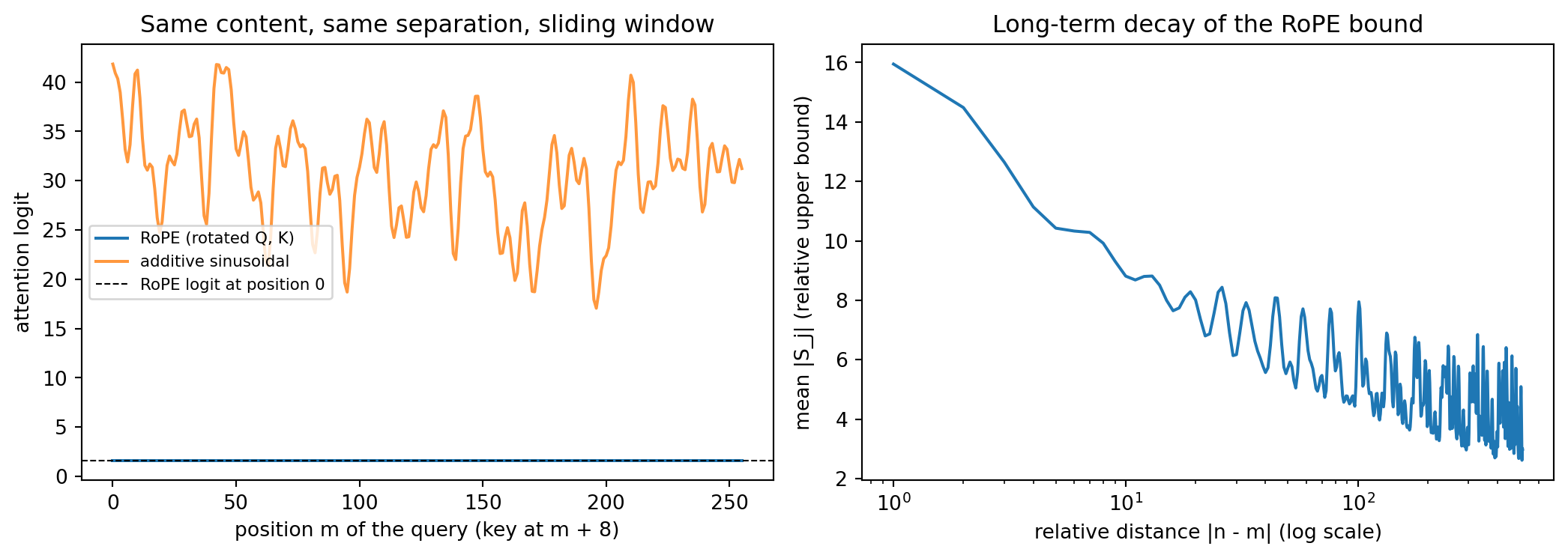
RoPE logit at offset 8, query position 0: 1.634715
Max deviation across 256 shifted positions: 0.00e+00
Additive sinusoidal logit range: [17.058, 41.833] (spread 24.775)
Relative bound at distance 1 / 64 / 512: 15.95 / 5.70 / 2.99
Figure 218.1: RoPE makes the attention logit a function of the relative offset alone. Left: the logit for a fixed content pair as both tokens slide along the sequence at constant separation, flat for RoPE and drifting for the additive sinusoidal scheme. Right: the Abel-summation bound of Su et al., the quantity that caps how large the logit contribution can be at a given relative distance, decaying as the distance grows.
The deviation figure is the point. Under RoPE the logit for a fixed content pair held at a fixed separation is invariant to where in the sequence that pair sits, exactly, while the additive scheme produces a logit that wanders over a range comparable to its own magnitude. The right panel plots the distance-dependent factor of the bound above, which falls by roughly a factor of five between adjacent tokens and tokens five hundred apart. Note what the panel is and is not: it is a ceiling fixed by the frequency ladder, not a measurement of realized attention, and it is exactly the term that context-extension recipes manipulate when they rescale \(\theta_i\) to keep the bound from collapsing past the trained length.
218.4.5 The Full Architecture
The encoder consists of \(N\) identical layers, each containing a multi-head self-attention sublayer followed by a position-wise feedforward network, with residual connections and layer normalization around each sublayer:
The feedforward network applies two linear transformations with a ReLU activation:
\[\text{FFN}(x) = \max(0, x W_1 + b_1) W_2 + b_2,\]
with the inner dimension typically four times the model dimension. The decoder adds a cross-attention sublayer between the self-attention and feedforward sublayers, where queries come from the decoder and keys and values come from the encoder output.
218.5 The Transition: From LSTM to Transformer Dominance
The period from 2015 to 2018 represents a transitional phase during which attention mechanisms were grafted onto recurrent architectures before eventually supplanting them. The shift can be traced through a sequence of landmark models.
ELMo (Peters et al., 2018) produced contextualized word representations by running a deep bidirectional LSTM over text and extracting hidden states from each layer. Its key insight—that the same word token should have different representations depending on context—proved enormously influential. Yet ELMo still depended on sequential LSTM computation, limiting the parallelism available during training.
BERT (Devlin et al., 2018) and GPT (Radford et al., 2018) both appeared in the same year and both adopted the transformer architecture exclusively, discarding the LSTM entirely. BERT used a bidirectional transformer encoder pretrained with masked language modeling and next sentence prediction, then fine-tuned on downstream tasks. GPT used a unidirectional transformer decoder pretrained with causal language modeling. Both achieved state-of-the-art results across a wide range of natural language benchmarks, definitively demonstrating that the recurrent inductive bias was not necessary for strong sequential performance and that the transformer’s parallelism advantage during training enabled scaling to larger datasets than LSTM-based models could efficiently exploit.
The retrospective explanation for why transformers superseded LSTMs combines several factors. First, full parallelism across sequence positions allows training throughput to scale with compute in a way sequential models cannot match. Second, the \(\mathcal{O}(1)\) maximum path length between any two positions in a single transformer layer fundamentally changes the optimization difficulty of learning long-range dependencies: gradient flows directly between any two positions without multiplicative attenuation through intermediate steps. Third, the attention mechanism provides an explicit, learned routing mechanism for information across the sequence, whereas the LSTM must compress all relevant context into the fixed-dimensional hidden state through nonlinear gates. Fourth, transformers scale more predictably with model size and data volume, as documented by subsequent scaling law research (Kaplan et al., 2020), making investment in larger models reliably productive in a way that larger LSTM stacks were not.
The CNN era established that depth and residual connectivity were key to learning hierarchical representations in vision. The RNN era demonstrated that sequential inductive bias could be encoded in learned gating mechanisms, but revealed the fundamental tension between expressiveness and training efficiency in sequential models. Attention resolved that tension by making the sequence-to-sequence routing function explicit, learnable, and fully parallelizable—and the transformer packaged these properties into an architecture that has dominated deep learning across modalities from 2018 to the present.
218.6 Reopening the Vertical Channel: Latent Feedback
The story told so far has a loose end. The RNN and the LSTM carried a full real-valued state vector from one step to the next, and that state was the whole point of the architecture: it was where the model kept whatever it had figured out but had not yet said. The transformer discarded that carry entirely. Section 5 justified the trade in terms of parallelism and path length, and the justification held, because the KV cache turned out to be a far better memory of the past than a single compressed vector. But the KV cache is a memory of what was written, not of what was computed. Every decoding step still builds a rich internal representation at the top of the stack and then throws it away, keeping only the one token it happened to sample. Wang et al. (2026) call the resulting design a partially blocked communication channel and propose closing it. Their full-bandwidth transformer feeds the previous top-layer hidden state back into the bottom of the stack alongside the sampled token embedding, fusing the two through a gated linear unit. The recurrent carry that the transformer gave up in 2017 comes back, but this time as a supplement to attention rather than a replacement for it.
218.6.1 Two axes, two very different bandwidths
An autoregressive decoder computes along two axes. Horizontally, across generated positions, dense causal attention lets the representation at step \(t\) read the keys and values of every earlier position, so the horizontal channel is wide and already well provisioned. Vertically, through model depth, each step transforms its input embedding through \(L\) layers to a top-layer state \(h_t \in \mathbb{R}^{d}\), then projects to logits and samples. The question is what crosses the boundary from step \(t\) to step \(t+1\) that was not already in the cache.
Fix notation. Let \(V\) be the vocabulary size, \(E \in \mathbb{R}^{V \times d}\) the embedding table, \(E[y]\) the row for token \(y\), \(W_u \in \mathbb{R}^{V \times d}\) the unembedding, and \(h_t \in \mathbb{R}^{d}\) the top-layer hidden state at step \(t\). In the standard decoder,
The KV cache entries for positions \(\le t\) are frozen functions of \(x_{\le t}\), so they carry no new information across the boundary; they are the record of past inputs, not of the current step’s work. The only genuinely new object crossing from step \(t\) into step \(t+1\) is \(y_t\), a single draw from a set of size \(V\). Its entropy is bounded by the log of that set size,
\[I_{\text{token}} \;=\; H(y_t) \;\le\; \log_2 V \text{ bits},\]
with equality only for a uniform predictive distribution, which never happens in a trained model. At \(V = 128{,}000\) that ceiling is \(16.97\) bits, and at \(V = 256{,}000\) it is \(17.97\) bits: doubling the vocabulary buys exactly one more bit. Meanwhile \(h_t\), which the model spent \(L\) layers of computation producing, is deleted.
How much does \(h_t\) hold? A real vector has unbounded entropy in exact arithmetic, so the honest way to size the channel is to ask how much survives noise. Model the usable content of \(h_t\) as \(d\) independent coordinates observed through additive Gaussian noise with per-coordinate signal-to-noise ratio \(\mathrm{SNR}\). The Shannon capacity of that channel is
\[I_{\text{latent}} \;=\; \frac{d}{2} \log_2\!\left(1 + \mathrm{SNR}\right) \text{ bits per step},\]
which for \(d = 4096\) and a modest \(\mathrm{SNR} = 10\) gives \(7{,}084.9\) bits, about \(417.6\) times the \(16.97\) bit token ceiling. The bound is conservative twice over: it assumes independent coordinates and it is far below the \(16d\) bits that a bfloat16 vector physically occupies. Even at \(\mathrm{SNR} = 1\), where each coordinate carries half a bit, the latent channel is two orders of magnitude wider than the token channel. The asymmetry is structural, and it does not shrink as models scale, because \(\log_2 V\) grows logarithmically in vocabulary size while \(d\) grows linearly with width.
flowchart LR
  subgraph STD["Standard decoding step"]
    direction TB
    A1["input x_t is a token embedding"] --> A2["layers 1 to L"]
    A2 --> A3["top hidden state h_t"]
    A3 --> A4["unembed and sample"]
    A3 --> A6["h_t is discarded"]
    A4 --> A5["sampled token y_t"]
    A5 -->|"at most log2 V bits"| A7["next input is the embedding of y_t"]
  end
  subgraph FBT["Full-bandwidth decoding step"]
    direction TB
    B1["input x_t is a fused vector"] --> B2["layers 1 to L"]
    B2 --> B3["top hidden state h_t"]
    B3 --> B4["unembed and sample"]
    B4 --> B5["sampled token y_t"]
    B3 -->|"order d real values"| B6["gated linear unit"]
    B5 -->|"at most log2 V bits"| B6
    B6 --> B7["next input carries both"]
  end
218.6.2 The gated fusion, and why nothing else has to change
Latent feedback replaces the next-input rule and nothing else. Concatenate the sampled token embedding with the previous top-layer state into \(u_t = [\,E[y_t] \,;\, h_t\,] \in \mathbb{R}^{2d}\) and form the next input with a gated linear unit,
with \(W_a, W_b \in \mathbb{R}^{d \times 2d}\), \(\sigma\) the logistic function, and \(\odot\) the elementwise product. The multiplicative branch \(\sigma(W_b u_t + b_b) \in (0,1)^d\) is a learned per-coordinate valve: it decides, coordinate by coordinate and step by step, how much of the latent carry to admit. That matters because the useful fraction of \(h_t\) varies enormously across steps, and an unmodulated addition would force the model to accept a fixed dose of a signal that is sometimes essential and sometimes pure interference.
Three properties follow directly from the form of the update.
The architecture is untouched.\(x_{t+1}\) has the same shape the layer stack always consumed. No layer, attention pattern, normalization, or head is modified. The added parameters are the two matrices \(W_a\) and \(W_b\), together \(2 \cdot (d \times 2d) = 4d^2\) entries, against roughly \(12 d^2\) per transformer layer (\(4d^2\) for the attention projections plus \(8d^2\) for the feedforward block). For a stack of \(L = 32\) layers the fusion adds \(4d^2 / (12 d^2 L) \approx 1.04\%\) to the parameter count.
The KV cache still works. The cache at layer \(\ell\) holds \(K^{(\ell)}_{\le t}\) and \(V^{(\ell)}_{\le t}\), which are functions of \(x_{\le t}\). Latent feedback determines \(x_{t+1}\), a new column, and leaves every earlier column untouched, so the cache remains strictly append-only and no past entry needs recomputation. The only extra work per decoded token is the fusion itself, about \(2 \cdot 4d^2 = 8d^2\) FLOPs against roughly \(2 \cdot 12 d^2 L = 24 d^2 L\) FLOPs for a full decode step, a ratio of \(1/(3L) \approx 1.04\%\) at \(L = 32\). This is the arithmetic behind the paper’s claim of negligible per-token decoding overhead.
The language-modeling objective is unchanged. Unrolling the recursion, \(h_t\) is a deterministic function of \(x_{\le t}\), which is a deterministic function of \(y_{<t}\) and the fixed initial state. So the conditional \(p(y_t \mid y_{<t}) = \mathrm{softmax}(W_u h_t)\) is still a genuine conditional on the token prefix, the chain rule \(\log p(y_{1:T}) = \sum_t \log p(y_t \mid y_{<t})\) still holds exactly, and the training loss is still plain cross entropy. There is no latent variable to marginalize, no auxiliary objective, no variational bound. This is what separates latent feedback from the long line of proposals that bolt a separate memory module onto a transformer: the model remains a normalized autoregressive language model over tokens.
One consequence of the same fact is worth naming, because it is a genuine constraint rather than a free lunch. Since \(h_t\) depends on the realized prefix, a training pass must feed the stack the states that the conditioning prefix would have produced. Teacher forcing supplies exactly that prefix, so the objective is consistent, but as Section 6.4 shows, computing those states is no longer free.
import torchtorch.manual_seed(3)d_model, d_emb, batch =512, 512, 4W_a = torch.randn(d_model, d_emb + d_model) / (d_emb + d_model) **0.5W_b = torch.randn(d_model, d_emb + d_model) / (d_emb + d_model) **0.5def latent_feedback_input(e_prev, h_prev, W_a, W_b):"""x_{t+1} = (W_a [E y_t ; h_t]) * sigmoid(W_b [E y_t ; h_t]).""" u = torch.cat([e_prev, h_prev], dim=-1)return (u @ W_a.T) * torch.sigmoid(u @ W_b.T)e_prev = torch.randn(batch, d_emb)h_prev = torch.randn(batch, d_model)x_next = latent_feedback_input(e_prev, h_prev, W_a, W_b)gate = torch.sigmoid(torch.cat([e_prev, h_prev], dim=-1) @ W_b.T)print(f"token embedding {tuple(e_prev.shape)} and hidden state {tuple(h_prev.shape)}")print(f"fused next input {tuple(x_next.shape)}, the shape the stack always consumed")print(f"mean gate value {gate.mean():.3f}, fraction of gates above 0.5: {(gate >0.5).float().mean():.3f}")# Zeroing the hidden-state columns recovers the standard decoder exactly.W_a0, W_b0 = W_a.clone(), W_b.clone()W_a0[:, d_emb:] =0.0W_b0[:, d_emb:] =0.0x_off_1 = latent_feedback_input(e_prev, h_prev, W_a0, W_b0)x_off_2 = latent_feedback_input(e_prev, torch.randn_like(h_prev), W_a0, W_b0)print(f"with the h columns zeroed, sensitivity to h_t: {(x_off_1 - x_off_2).abs().max():.1e}")
token embedding (4, 512) and hidden state (4, 512)
fused next input (4, 512), the shape the stack always consumed
mean gate value 0.495, fraction of gates above 0.5: 0.493
with the h columns zeroed, sensitivity to h_t: 0.0e+00
usingLinearAlgebra, Randomsigmoid(z) =1/ (1+exp(-z))""" latent_feedback_input(e_prev, h_prev, W_a, W_b)Fuse the sampled token embedding with the previous top-layer hidden state:`x_next = (W_a * u) .* sigmoid.(W_b * u)` where `u = [e_prev; h_prev]`.Columns are examples, so `e_prev` is `d_emb x batch`."""functionlatent_feedback_input(e_prev::AbstractMatrix, h_prev::AbstractMatrix, W_a::AbstractMatrix, W_b::AbstractMatrix) u =vcat(e_prev, h_prev)return (W_a * u) .*sigmoid.(W_b * u)endRandom.seed!(3)d_model, d_emb, batch =512, 512, 4scale =1/sqrt(d_emb + d_model)W_a =randn(d_model, d_emb + d_model) .* scaleW_b =randn(d_model, d_emb + d_model) .* scalee_prev =randn(d_emb, batch)h_prev =randn(d_model, batch)x_next =latent_feedback_input(e_prev, h_prev, W_a, W_b)gate =sigmoid.(W_b *vcat(e_prev, h_prev))println("fused next input size: ", size(x_next))println("mean gate value: ", round(sum(gate) /length(gate), digits =3))
usendarray::{concatenate, Array2, Axis};fn sigmoid(z:f32) ->f32{1.0/ (1.0+ (-z).exp())}/// Fuse the sampled token embedding with the previous top-layer hidden state./// `e_prev` is [batch, d_emb], `h_prev` is [batch, d_model], and both weight/// matrices are [d_model, d_emb + d_model]. Returns [batch, d_model].fn latent_feedback_input( e_prev:&Array2<f32>, h_prev:&Array2<f32>, w_a:&Array2<f32>, w_b:&Array2<f32>,) -> Array2<f32>{let u = concatenate(Axis(1),&[e_prev.view(), h_prev.view()]).expect("embedding and hidden state must share a batch dimension");let linear = u.dot(&w_a.t());let gate = u.dot(&w_b.t()).mapv(sigmoid); linear * gate}fn main() {let (batch, d_emb, d_model) = (4usize,512usize,512usize);let e_prev =Array2::<f32>::zeros((batch, d_emb));let h_prev =Array2::<f32>::zeros((batch, d_model));let w_a =Array2::<f32>::zeros((d_model, d_emb + d_model));let w_b =Array2::<f32>::zeros((d_model, d_emb + d_model));let x_next = latent_feedback_input(&e_prev,&h_prev,&w_a,&w_b);println!("fused next input shape: {:?}", x_next.dim());}
The Python tab prints a mean gate value of \(0.495\) with \(49.3\%\) of gates open at initialization, which is the neutral starting point a symmetric random \(W_b\) should give. The last check is the one that matters for the training schedule: zeroing the \(h\) columns of \(W_a\) and \(W_b\) makes the fused input completely insensitive to \(h_t\), with a measured maximum deviation of exactly \(0.0\). The standard transformer is therefore a point in the full-bandwidth parameter space, not a different model, and the feedback channel can be opened continuously from zero rather than switched on discontinuously.
218.6.3 A renewed depth budget
The bandwidth argument explains what latent feedback can transmit. A separate argument explains why the model has anything worth transmitting, and it concerns depth.
In a standard decoder, attention at layer \(\ell\) of position \(t\) reads the keys and values produced at layer \(\ell - 1\) of positions \(\le t\). Information can therefore move sideways at any layer, but it can only move upward one layer at a time, and it never moves back down. The longest chain of nonlinear transformations between any input embedding and any output logit is exactly \(L\), independent of how many tokens separate them. This is the well-known observation that a transformer is a constant-depth circuit in the sequence length: attention buys unlimited horizontal reach at zero depth cost, and buys no depth at all.
The only escape in a standard model is to write intermediate results out as tokens and read them back in. That is precisely what a chain of thought is: a depth extension mechanism that pays for each additional \(L\) layers of serial computation by emitting a token, and therefore by squeezing the entire intermediate state through the \(\log_2 V\) bit aperture of Section 6.1. Latent feedback provides the same depth extension without the aperture. Because \(h_t\) is produced at depth \(L\) and injected at depth \(0\) of step \(t+1\), a computational path spanning \(m\) consecutive decoding steps has effective depth
\[D_{\text{eff}}(m) \;=\; m L,\]
against \(D_{\text{eff}} = L\) for any \(m\) in the standard model. Depth becomes a function of generated length as well as layer count, and the marginal cost of the next \(L\) layers of serial computation is one decoding step whose content the model no longer has to verbalize. This is the mechanism behind the paper’s report that full-bandwidth models produce shorter reasoning traces at equal or better accuracy: work that previously had to be written down in order to survive to the next step can now stay latent.
218.6.4 The training problem, and the cost of a \(k\)-pass objective
Section 5 credited the transformer’s victory to parallel teacher forcing, so any proposal that breaks it is proposing to undo the transition. Latent feedback breaks it. Under teacher forcing in a standard decoder, every input \(x_t = E[y_{t-1}]\) is known from the training text before the forward pass begins, so all \(T\) positions are processed in one batched call and the sequential depth of a training step is \(\mathcal{O}(1)\) in \(T\). With latent feedback, \(x_{t+1}\) depends on \(h_t\), which is an output of the forward pass at step \(t\). An exact implementation would therefore require \(T\) sequential stack evaluations per training sequence, restoring precisely the \(\mathcal{O}(T)\) serial bottleneck that made LSTM training slow.
The resolution is to note that the recursion can be unrolled to a fixed number of levels and each level evaluated in parallel. Define a sequence of passes indexed by \(k\):
Pass \(1\) is an ordinary transformer forward pass with no feedback. Once \(h^{(1)}\) is known for every position, the inputs \(x^{(2)}_t\) for every position are known too, so pass \(2\) is again fully parallel across \(t\), and so on. Each additional pass extends the feedback by one decoding step, and \(k = T\) recovers the exact serial recursion. Wang et al. (2026) train with a scheduled multi-pass objective: latent feedback is introduced late in pretraining rather than from initialization, and a small fraction of batches use a deeper feedback pass for stability.
The cost is easy to account for. Let \(F\) be the FLOP cost of one forward pass over a training sequence, so that backpropagation costs about \(2F\) and an ordinary training step costs \(3F\). Running the first \(k-1\) passes without gradient tracking and backpropagating only through the last gives
So \(M_1 = 1\), \(M_2 = 4/3 \approx 1.333\), and \(M_3 = 5/3 \approx 1.667\). If a fraction \(\rho\) of latent-phase batches use three passes and the rest use two, the phase multiplier is \((1-\rho) M_2 + \rho M_3\), and if the latent phase covers the last fraction \(\phi\) of pretraining, the whole-run multiplier is \((1 - \phi) + \phi\bigl[(1-\rho) M_2 + \rho M_3\bigr]\). The cell below evaluates this at the illustrative values \(\phi = 0.20\) and \(\rho = 0.10\); the paper does not publish these constants, so treat the resulting figures as an accounting exercise in the shape of the described schedule rather than as reported measurements.
218.6.5 Measuring the channel and the mechanism
The cell below does three things. First it tabulates the two channel widths from Section 6.1. Then it isolates the mechanism on a task built so that the missing bits are the only obstacle. A hidden phase \(z_t \in [0,1)\) evolves as \(z_t = (z_{t-1} + a_t) \bmod 1\) with increments \(a_t \sim \mathrm{Uniform}[0,1)\) revealed one per step, and the model must emit the bucket \(y_t = \lfloor V_b z_t \rfloor\) with \(V_b = 4\). Two loops are trained on it under teacher forcing. The token-only loop receives just \(E[y_{t-1}]\), the best case for a standard decoder since the true previous token is supplied. The latent-feedback loop receives \(\mathrm{GLU}(E[y_{t-1}], h_{t-1})\). Finally the cell evaluates the compute accounting of Sections 6.2 and 6.4.
The token-only loop has an exact Bayes floor worth deriving, because it makes the demonstration falsifiable rather than anecdotal. Conditioned on \(y_{t-1} = b\), the phase \(z_{t-1}\) is uniform on \([b/V_b, (b+1)/V_b)\), so given the observed increment \(a_t\) the next phase \(z_t\) is uniform on an arc of width \(1/V_b\) beginning at \(c = (b/V_b + a_t) \bmod 1\). That arc meets at most two buckets, splitting its mass as \(p\) and \(1-p\) with
\[p = V_b\left(\frac{\lceil c V_b \rceil}{V_b} - c\right),\]
and since \(a_t\) is uniform and independent, \(c\) is uniform on \([0,1)\) and therefore \(p\) is uniform on \((0,1)\). The conditional entropy in nats is \(H(p) = -p \ln p - (1-p)\ln(1-p)\), so the achievable cross entropy is
using \(\int_0^1 p \ln p \,\mathrm{d}p = \left[\tfrac{p^2}{2}\ln p - \tfrac{p^2}{4}\right]_0^1 = -\tfrac{1}{4}\). Notice that the floor does not depend on \(V_b\): making the emitted vocabulary finer shrinks the arc and the buckets together. The latent loop has no such floor, because \(z_{t-1}\) is one real number and \(h_{t-1}\) carries \(d\) of them, so its achievable loss is zero. One caveat stated plainly: a real transformer could in principle recover \(z_t\) by attending to all past increments in the KV cache, and the toy forbids that by giving each step a fixed two-layer stack and only the current increment. That restriction is the finite-depth analogue of Section 6.3, where re-deriving a \(t\)-step accumulation needs more serial depth than \(L\) layers provide.
Code
import numpy as npimport torchimport torch.nn as nnimport matplotlib.pyplot as plttorch.manual_seed(0)rng = np.random.default_rng(0)# === Part A: bits crossing one step boundaryVOCABS = [32_000, 50_257, 128_000, 256_000]DIMS = [512, 1024, 2048, 4096, 8192]SNR =10.0# usable signal-to-noise ratio per latent coordinatedef latent_bits(d, snr=SNR):return0.5* d * np.log2(1.0+ snr)print("token-only channel: one sampled token per step")for V in VOCABS:print(f" V = {V:>7,} log2(V) = {np.log2(V):6.2f} bits")ref = np.log2(128_000)print("\nlatent-feedback channel: Gaussian capacity of h_t, SNR = 10")for d in DIMS: b = latent_bits(d)print(f" d = {d:>5} capacity = {b:9.1f} bits ratio to log2(128000) = {b / ref:7.1f}x")# === Part B: a toy loop where the extra bits are decisiveV_BUCKET =4# emitted vocabulary: four coarse buckets of the unit circleD_EMB =16# token embedding widthD_HID =64# width of the stackD_FUSE =16# width of the fused next-step inputT =16# decoding steps per rolloutBATCH =128STEPS =220LR =8e-3def make_batch(batch=BATCH, steps=T, gen=None): a = torch.rand(batch, steps, generator=gen) # increment revealed at step t z0 = torch.rand(batch, 1, generator=gen) z = (z0 + torch.cumsum(a, dim=1)) %1.0# phase after each step y = torch.clamp((z * V_BUCKET).long(), max=V_BUCKET -1) z_prev = torch.cat([z0, z[:, :-1]], dim=1) y_prev = torch.clamp((z_prev * V_BUCKET).long(), max=V_BUCKET -1) feats = torch.stack([torch.cos(2* np.pi * a), torch.sin(2* np.pi * a)], dim=-1)return feats, y_prev, yclass Stack(nn.Module):"""The shared model stack: fused input plus this step's observation, then logits."""def__init__(self, d_in):super().__init__()self.body = nn.Sequential( nn.Linear(d_in +2, D_HID), nn.Tanh(), nn.Linear(D_HID, D_HID), nn.Tanh(), )self.head = nn.Linear(D_HID, V_BUCKET)def forward(self, x, obs): h =self.body(torch.cat([x, obs], dim=-1))return h, self.head(h)class TokenOnly(nn.Module):"""Only the sampled token returns to the bottom of the stack."""def__init__(self):super().__init__()self.emb = nn.Embedding(V_BUCKET, D_EMB)self.stack = Stack(D_EMB)def forward(self, feats, y_prev): logits = []for t inrange(feats.shape[1]): x =self.emb(y_prev[:, t]) _, lg =self.stack(x, feats[:, t]) logits.append(lg)return torch.stack(logits, dim=1)class LatentFeedback(nn.Module):"""The top-layer hidden state is fused with the token embedding by a GLU."""def__init__(self):super().__init__()self.emb = nn.Embedding(V_BUCKET, D_EMB)self.W_a = nn.Linear(D_EMB + D_HID, D_FUSE)self.W_b = nn.Linear(D_EMB + D_HID, D_FUSE)self.stack = Stack(D_FUSE)self.h0 = nn.Parameter(torch.zeros(D_HID))def fuse(self, e, h): u = torch.cat([e, h], dim=-1)returnself.W_a(u) * torch.sigmoid(self.W_b(u))def forward(self, feats, y_prev): h =self.h0.expand(feats.shape[0], D_HID) logits = []for t inrange(feats.shape[1]): x =self.fuse(self.emb(y_prev[:, t]), h) h, lg =self.stack(x, feats[:, t]) logits.append(lg)return torch.stack(logits, dim=1)loss_fn = nn.CrossEntropyLoss()def train(model, tag): opt = torch.optim.Adam(model.parameters(), lr=LR) gen = torch.Generator().manual_seed(1234) curve = []for _ inrange(STEPS): feats, y_prev, y = make_batch(gen=gen) loss = loss_fn(model(feats, y_prev).reshape(-1, V_BUCKET), y.reshape(-1)) opt.zero_grad() loss.backward() opt.step() curve.append(loss.item()) gen_eval = torch.Generator().manual_seed(99)with torch.no_grad(): feats, y_prev, y = make_batch(batch=2048, gen=gen_eval) logits = model(feats, y_prev) held = loss_fn(logits.reshape(-1, V_BUCKET), y.reshape(-1)).item() acc = (logits.argmax(-1) == y).float().mean().item() n_par =sum(p.numel() for p in model.parameters())print(f"{tag:16s} params={n_par:6d} held-out loss={held:.4f} nats accuracy={acc:.3f}")return np.array(curve), held, accprint()tok_curve, tok_loss, tok_acc = train(TokenOnly(), "token-only")lat_curve, lat_loss, lat_acc = train(LatentFeedback(), "latent-feedback")u = rng.random(400_000)p = np.clip((np.ceil(u * V_BUCKET) / V_BUCKET - u) * V_BUCKET, 1e-12, 1-1e-12)mc_floor =float(np.mean(-p * np.log(p) - (1- p) * np.log(1- p)))print(f"\nanalytic token-only floor = 0.5000 nats, Monte Carlo = {mc_floor:.4f} nats")print(f"token-only gap to that floor = {tok_loss -0.5:+.4f} nats")print(f"latent-feedback loss is {lat_loss / tok_loss:.3f} of the token-only loss")# === Part C: what the wider channel costsL =32# transformer layersPHI =0.20# fraction of pretraining run with latent feedback onRHO =0.10# fraction of latent-phase batches using a third passDATA_RATIO =1.5# baseline needs this many more tokens to matchparam_overhead =4.0/ (12.0* L) # two GLU matrices against 12 d^2 per layerdecode_overhead =1.0/ (3.0* L) # GLU FLOPs against a full decode steppass2, pass3 = (2+2) /3, (3+2) /3# cost multiplier of a k-pass training stepphase_mult = (1- RHO) * pass2 + RHO * pass3train_mult = (1- PHI) + PHI * phase_multtotal_mult = train_mult * (1+ param_overhead)saving =1.0- total_mult / DATA_RATIOprint(f"\nGLU parameter overhead at L = {L}: {param_overhead:.2%}")print(f"per-token decode FLOP overhead: {decode_overhead:.2%}")print(f"latent-phase training multiplier: {phase_mult:.3f}")print(f"whole-run training multiplier: {train_mult:.3f}")print(f"with parameter overhead: {total_mult:.3f}")print(f"pretraining compute saved vs a {DATA_RATIO}x-token baseline: {saving:.1%}")fig, axes = plt.subplots(1, 2, figsize=(10.5, 4.0))ax = axes[0]ax.axhspan(np.log2(min(VOCABS)), np.log2(max(VOCABS)), color="gray", alpha=0.35)ax.text(DIMS[0], np.log2(max(VOCABS)) *1.6,"token-only channel: log2(V), V from 32k to 256k", fontsize=8, color="dimgray")ax.plot(DIMS, [latent_bits(d) for d in DIMS], marker="o", label="latent feedback, SNR 10")ax.plot(DIMS, [latent_bits(d, 1.0) for d in DIMS], marker="s", label="latent feedback, SNR 1")ax.set_yscale("log")ax.set_xscale("log", base=2)ax.set_xlabel("model width d")ax.set_ylabel("bits crossing one step boundary")ax.set_title("Inter-step channel capacity")ax.legend(frameon=False, fontsize=8)ax = axes[1]w =15smooth =lambda c: np.convolve(c, np.ones(w) / w, mode="valid")ax.plot(smooth(tok_curve), label="token-only feedback")ax.plot(smooth(lat_curve), label="latent feedback")ax.axhline(0.5, ls="dashed", lw=1.2, color="gray")ax.text(len(tok_curve) *0.42, 0.54, "Bayes floor for token-only, 0.5 nats", fontsize=8, color="dimgray")ax.set_xlabel("training step")ax.set_ylabel("cross entropy (nats)")ax.set_title("Toy accumulator, 16 decoding steps")ax.legend(frameon=False, fontsize=8)fig.tight_layout()plt.show()
token-only channel: one sampled token per step
  V =  32,000   log2(V) =  14.97 bits
  V =  50,257   log2(V) =  15.62 bits
  V = 128,000   log2(V) =  16.97 bits
  V = 256,000   log2(V) =  17.97 bits

latent-feedback channel: Gaussian capacity of h_t, SNR = 10
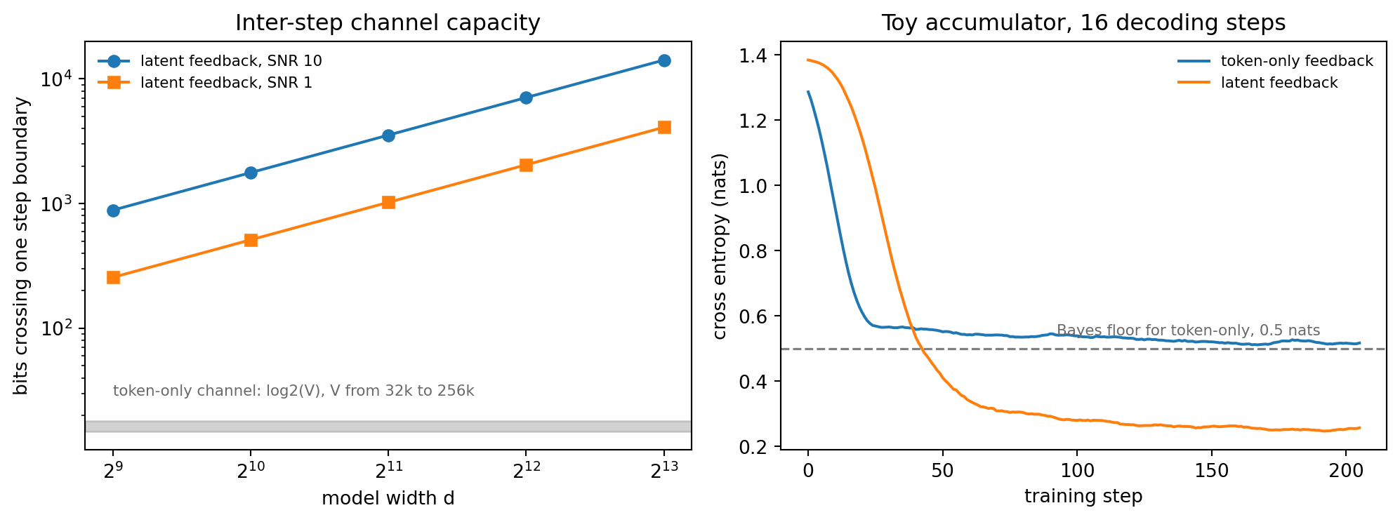
  d =   512   capacity =     885.6 bits   ratio to log2(128000) =    52.2x
  d =  1024   capacity =    1771.2 bits   ratio to log2(128000) =   104.4x
  d =  2048   capacity =    3542.5 bits   ratio to log2(128000) =   208.8x
  d =  4096   capacity =    7084.9 bits   ratio to log2(128000) =   417.6x
  d =  8192   capacity =   14169.8 bits   ratio to log2(128000) =   835.2x

token-only       params=  5700  held-out loss=0.5160 nats  accuracy=0.745
latent-feedback  params=  8356  held-out loss=0.2494 nats  accuracy=0.896

analytic token-only floor = 0.5000 nats, Monte Carlo = 0.4999 nats
token-only gap to that floor = +0.0160 nats
latent-feedback loss is 0.483 of the token-only loss

GLU parameter overhead at L = 32: 1.04%
per-token decode FLOP overhead:  1.04%
latent-phase training multiplier: 1.367
whole-run training multiplier:    1.073
with parameter overhead:          1.085
pretraining compute saved vs a 1.5x-token baseline: 27.7%
Figure 218.2: Left: bits crossing one decoding-step boundary, comparing the token-only channel (log2 of the vocabulary size) against the Gaussian capacity of a d-dimensional latent carry. Right: teacher-forced training curves on the toy phase accumulator, with the analytic Bayes floor for token-only feedback marked at 0.5 nats.
The toy result is clean. The token-only loop, with \(5{,}700\) parameters, converges to a held-out cross entropy of \(0.5160\) nats and \(74.5\%\) bucket accuracy, sitting \(0.0160\) nats above the analytic floor of \(0.5\) nats that the Monte Carlo estimate confirms at \(0.4999\). It has learned essentially everything its channel permits, and no amount of further training will move it, because the missing information was destroyed at the previous step’s sampling operation. The latent-feedback loop, with \(8{,}356\) parameters, reaches \(0.2494\) nats and \(89.6\%\) accuracy, which is \(48.3\%\) of the token-only loss and comfortably below a floor that is unbreakable for the other arm. The right panel of the figure shows the two curves separating exactly where the token-only arm meets the dashed line. The interpretive discipline here matters: the latent arm is not better because it is bigger or because it trained longer. It is better because it is on the far side of an information-theoretic barrier that the token-only arm cannot cross at any parameter count.
The cost side, from Part C at \(L = 32\), is that the fusion adds \(1.04\%\) to parameters and \(1.04\%\) to per-token decode FLOPs, while the illustrative schedule of Section 6.4 gives a latent-phase training multiplier of \(1.367\) and a whole-run multiplier of \(1.073\), or \(1.085\) once the extra parameters are counted. Set that against the headline result. Wang et al. (2026) train 1B-parameter models on up to 400B tokens and find that full-bandwidth models match or approach standard transformers trained on roughly \(1.5\times\) more tokens, with gains on validation loss, 5-shot evaluation, math and code generation, and instruction-tuned performance. Using the standard estimate \(C \approx 6ND\) for pretraining FLOPs with \(N\) parameters and \(D\) tokens, the baseline needs \(C_{\text{base}} = 6N(1.5D) = 9ND\) where the full-bandwidth model needs \(C_{\text{fb}} = 1.085 \times 6ND = 6.51ND\), a saving of \(27.7\%\) of pretraining compute at equal quality. The multi-pass overhead eats roughly a sixth of the nominal one-third saving and leaves the rest intact.
218.6.6 What this says about the arc
Read against Sections 2 through 5, latent feedback is a correction rather than a reversal. The transformer was right to abandon the recurrent hidden state as the primary memory of the past, because attention over a cache is a strictly better instrument for that job: it is content-addressed, lossless, and parallel, where a hidden state is compressed, lossy, and serial. What the transformer got wrong was throwing away the recurrent state as a carrier of work in progress, a role attention was never able to fill because attention reads what was written, not what was thought. Latent feedback restores that second role only, and pays for it with a \(\mathcal{O}(k)\) training multiplier and a per-token decode overhead near one percent rather than with the \(\mathcal{O}(T)\) serialization that made LSTMs uncompetitive.
The right frame is therefore that the 2017 architecture made two separable decisions and the field has since only relitigated one of them. Dropping recurrence for horizontal context was correct and has survived a decade of pressure. Dropping it for vertical carry was an unexamined side effect of the same change, and it left a channel roughly two orders of magnitude narrower than the hardware was already paying to compute. Sections 6.1 through 6.3 are the argument that this narrowing was never load-bearing; Section 6.4 is the argument that widening it is affordable. The open questions are the ones the paper is candid about: whether the multi-pass approximation stays faithful at \(k\) far below \(T\) for much longer generations, whether the benefit survives at scales well past 1B parameters, and whether a feedback path that carries non-verbalized computation makes chain-of-thought monitoring harder in precisely the cases where it is most wanted.
218.7 References
Krizhevsky, A., Sutskever, I., and Hinton, G. E. (2012). ImageNet classification with deep convolutional neural networks. Advances in Neural Information Processing Systems, 25. https://proceedings.neurips.cc/paper/2012/hash/c399862d3b9d6b76c8436e924a68c45b-Abstract.html
Simonyan, K. and Zisserman, A. (2014). Very deep convolutional networks for large-scale image recognition. arXiv:1409.1556. https://arxiv.org/abs/1409.1556
He, K., Zhang, X., Ren, S., and Sun, J. (2016). Deep residual learning for image recognition. Proceedings of the IEEE Conference on Computer Vision and Pattern Recognition (CVPR), 770–778. arXiv:1512.03385. https://arxiv.org/abs/1512.03385
Hochreiter, S. and Schmidhuber, J. (1997). Long short-term memory. Neural Computation, 9(8), 1735–1780. https://doi.org/10.1162/neco.1997.9.8.1735
Cho, K., van Merrienboer, B., Gulcehre, C., Bahdanau, D., Bougares, F., Schwenk, H., and Bengio, Y. (2014). Learning phrase representations using RNN encoder-decoder for statistical machine translation. arXiv:1406.1078. https://arxiv.org/abs/1406.1078
Sutskever, I., Vinyals, O., and Le, Q. V. (2014). Sequence to sequence learning with neural networks. Advances in Neural Information Processing Systems, 27. https://arxiv.org/abs/1409.3215
Bahdanau, D., Cho, K., and Bengio, Y. (2015). Neural machine translation by jointly learning to align and translate. International Conference on Learning Representations. arXiv:1409.0473. https://arxiv.org/abs/1409.0473
Vaswani, A., Shazeer, N., Parmar, N., Uszkoreit, J., Jones, L., Gomez, A. N., Kaiser, L., and Polosukhin, I. (2017). Attention is all you need. Advances in Neural Information Processing Systems, 30. https://proceedings.neurips.cc/paper/2017/hash/3f5ee243547dee91fbd053c1c4a845aa-Abstract.html
Peters, M. E., Neumann, M., Iyyer, M., Gardner, M., Clark, C., Lee, K., and Zettlemoyer, L. (2018). Deep contextualized word representations. arXiv:1802.05365. https://arxiv.org/abs/1802.05365
Devlin, J., Chang, M.-W., Lee, K., and Toutanova, K. (2018). BERT: Pre-training of deep bidirectional transformers for language understanding. arXiv:1810.04805. https://arxiv.org/abs/1810.04805
Radford, A., Narasimhan, K., Salimans, T., and Sutskever, I. (2018). Improving language understanding by generative pre-training. OpenAI Technical Report. https://openai.com/research/language-unsupervised
Kaplan, J., McCandlish, S., Henighan, T., Brown, T. B., Chess, B., Child, R., Gray, S., Radford, A., Wu, J., and Amodei, D. (2020). Scaling laws for neural language models. arXiv:2001.08361. https://arxiv.org/abs/2001.08361
Su, J., Ahmed, M., Lu, Y., Pan, S., Bo, W., and Liu, Y. (2024). RoFormer: Enhanced transformer with rotary position embedding. Neurocomputing, 568, 127063. https://doi.org/10.1016/j.neucom.2023.127063
Wang, X., Cai, Z., Zhan, Z., Dong, H., Fan, Y., de Rosa, G., Pearce, T., and Langford, J. (2026). Full-bandwidth transformer. arXiv:2608.08888. https://arxiv.org/abs/2608.08888
Wang, Xi, Ziyang Cai, Zheng Zhan, Harry Dong, Ying Fan, Gustavo de Rosa, Tim Pearce, and John Langford. 2026. “Full-Bandwidth Transformer.”arXiv Preprint arXiv:2608.08888.
Source Code
# The Road to Transformers {#sec-road-to-transformers}The transformer architecture, introduced in 2017, did not emerge from a vacuum. It was the culmination of two decades of increasingly sophisticated neural sequence models, each generation exposing the limitations of its predecessor and pointing toward what the next would need to solve. Understanding this lineage is not merely historical: the problems that motivated each transition---vanishing gradients, sequential bottlenecks, fixed-length representation, quadratic attention cost---remain live engineering concerns in every deployment of modern language and vision systems.## The CNN Era and Residual ConnectionsConvolutional neural networks demonstrated that depth was the key ingredient for representational power in vision tasks. AlexNet (Krizhevsky et al., 2012) showed that a five-layer convolutional network trained on GPU hardware could dramatically outperform hand-engineered features on ImageNet, reducing top-5 error from roughly 26% to 15.3%. VGGNet (Simonyan and Zisserman, 2014) pushed this further by using very small $3 \times 3$ convolution kernels stacked in deep configurations of 16 to 19 layers, demonstrating that depth itself, rather than large receptive fields, drove performance.The natural question was: why not go deeper? The empirical answer was troubling. Networks deeper than about 20 layers trained worse than shallower ones---not because of overfitting, but because of the vanishing gradient problem. During backpropagation, gradients are multiplied layer by layer via the chain rule. If each multiplication attenuates the signal, the gradient reaching early layers is exponentially smaller than the loss gradient at the output, making early-layer weights nearly untrainable.He et al. (2016) solved this with the residual connection, a deceptively simple modification. Instead of learning a direct mapping $\mathcal{H}(x)$ from input to output, a residual block learns only the residual $\mathcal{F}(x) = \mathcal{H}(x) - x$, so the full transformation is$$\mathcal{H}(x) = \mathcal{F}(x) + x.$$The addition of the identity shortcut $x$ creates an alternative path for gradient flow. During backpropagation through a residual block, the gradient of the loss $\mathcal{L}$ with respect to the block input satisfies$$\frac{\partial \mathcal{L}}{\partial x} = \frac{\partial \mathcal{L}}{\partial \mathcal{H}} \cdot \left(1 + \frac{\partial \mathcal{F}}{\partial x}\right).$$The additive $1$ in the gradient ensures that even if $\partial \mathcal{F}/\partial x$ vanishes, a unit-magnitude gradient flows unimpeded through the skip connection back to all earlier layers. This allowed He et al. to train networks of 152 layers---ResNet-152---achieving 3.57% top-5 error on ImageNet, surpassing human-level performance on that benchmark. The deeper architectural insight is that residual connections make the optimization landscape substantially easier to traverse, a property later confirmed by loss landscape visualization work.```pythonimport torchimport torch.nn as nnimport torch.nn.functional as Fclass ResidualBlock(nn.Module):def__init__(self, channels: int):super().__init__()self.conv1 = nn.Conv2d(channels, channels, kernel_size=3, padding=1, bias=False)self.bn1 = nn.BatchNorm2d(channels)self.conv2 = nn.Conv2d(channels, channels, kernel_size=3, padding=1, bias=False)self.bn2 = nn.BatchNorm2d(channels)def forward(self, x: torch.Tensor) -> torch.Tensor: residual = x out = F.relu(self.bn1(self.conv1(x))) out =self.bn2(self.conv2(out))return F.relu(out + residual)torch.manual_seed(0)block = ResidualBlock(channels=16)x = torch.randn(2, 16, 8, 8)y = block(x)y.sum().backward()grad_norm = x.grad.norm().item() if x.requires_grad elseNonex_req = torch.randn(2, 16, 8, 8, requires_grad=True)y_req = block(x_req)y_req.sum().backward()print(f"Input shape: {x_req.shape}, Output shape: {y_req.shape}")print(f"Input gradient norm: {x_req.grad.norm().item():.4f}")```## The RNN and LSTM EraWhile CNNs reshaped computer vision, sequence modeling required a different inductive bias: the ability to process variable-length inputs where the order of elements carried meaning. Recurrent neural networks (RNNs) addressed this by maintaining a hidden state that accumulated information across time steps. The vanilla RNN update at time step $t$ is$$h_t = \tanh(W_h h_{t-1} + W_x x_t + b),$$where $h_t \in \mathbb{R}^d$ is the hidden state, $x_t \in \mathbb{R}^m$ is the input, and $W_h$, $W_x$ are weight matrices. The same parameters are reused at every step, giving the model a compact representation of sequential inductive bias.The fundamental weakness of the vanilla RNN mirrors the deep CNN problem: vanishing gradients through time. The gradient of the loss with respect to an early hidden state $h_k$ involves the product$$\frac{\partial \mathcal{L}}{\partial h_k} = \frac{\partial \mathcal{L}}{\partial h_T} \prod_{t=k+1}^{T} \frac{\partial h_t}{\partial h_{t-1}}.$$Each factor $\partial h_t / \partial h_{t-1} = \text{diag}(\tanh'(\cdot)) W_h$ has singular values that, for most initializations, are less than one. Over a sequence of length $T$, the product decays exponentially and early-step gradients vanish, preventing the model from learning long-range dependencies. Additionally, vanilla RNNs are inherently sequential: computing $h_t$ requires $h_{t-1}$, preventing parallelization across time steps during training.### Long Short-Term MemoryHochreiter and Schmidhuber (1997) proposed the Long Short-Term Memory (LSTM) to address the vanishing gradient problem through a gating mechanism that provides a nearly constant error carousel. The LSTM maintains two state vectors: a cell state $c_t \in \mathbb{R}^d$ that acts as a long-term memory, and a hidden state $h_t \in \mathbb{R}^d$ that serves as the working output. The update equations are$$f_t = \sigma(W_f [h_{t-1}, x_t] + b_f) \quad \text{(forget gate)},$$$$i_t = \sigma(W_i [h_{t-1}, x_t] + b_i) \quad \text{(input gate)},$$$$\tilde{c}_t = \tanh(W_c [h_{t-1}, x_t] + b_c) \quad \text{(candidate cell)},$$$$c_t = f_t \odot c_{t-1} + i_t \odot \tilde{c}_t \quad \text{(cell update)},$$$$o_t = \sigma(W_o [h_{t-1}, x_t] + b_o) \quad \text{(output gate)},$$$$h_t = o_t \odot \tanh(c_t).$$The crucial innovation is the cell state update $c_t = f_t \odot c_{t-1} + i_t \odot \tilde{c}_t$. When the forget gate is close to one and the input gate is close to zero, $c_t \approx c_{t-1}$: information flows forward through time with gradient magnitude near one. This creates a highway for gradient flow analogous to the residual connection in ResNet, but adaptive: the gates themselves are learned from data, allowing the network to decide what to retain, update, or erase.Cho et al. (2014) introduced the Gated Recurrent Unit (GRU) as a streamlined variant that merges the forget and input gates into a single update gate $z_t$ and eliminates the separate cell state, reducing parameter count while retaining much of the LSTM's capacity for long-range memory.```pythonimport torchimport torch.nn as nntorch.manual_seed(42)vocab_size =20embed_dim =16hidden_dim =32seq_len =10batch_size =8X = torch.randint(0, vocab_size, (batch_size, seq_len))y = (X.float().mean(dim=1) > vocab_size /2).long()embedding = nn.Embedding(vocab_size, embed_dim)lstm = nn.LSTM(embed_dim, hidden_dim, batch_first=True)classifier_lstm = nn.Linear(hidden_dim, 2)classifier_avg = nn.Linear(embed_dim, 2)optimizer_lstm = torch.optim.Adam(list(embedding.parameters()) +list(lstm.parameters()) +list(classifier_lstm.parameters()), lr=1e-2)optimizer_avg = torch.optim.Adam(list(embedding.parameters()) +list(classifier_avg.parameters()), lr=1e-2)loss_fn = nn.CrossEntropyLoss()for step inrange(200): emb = embedding(X) out, (h_n, _) = lstm(emb) logits_lstm = classifier_lstm(h_n.squeeze(0)) loss_lstm = loss_fn(logits_lstm, y) optimizer_lstm.zero_grad() loss_lstm.backward() optimizer_lstm.step() logits_avg = classifier_avg(emb.mean(dim=1)) loss_avg = loss_fn(logits_avg, y) optimizer_avg.zero_grad() loss_avg.backward() optimizer_avg.step()with torch.no_grad(): emb = embedding(X) _, (h_n, _) = lstm(emb) acc_lstm = (classifier_lstm(h_n.squeeze(0)).argmax(1) == y).float().mean().item() acc_avg = (classifier_avg(emb.mean(dim=1)).argmax(1) == y).float().mean().item()print(f"LSTM accuracy: {acc_lstm:.2f}")print(f"Mean-pooling accuracy: {acc_avg:.2f}")```Despite LSTMs' success on tasks requiring hundreds of time steps of memory---machine translation, speech recognition, language modeling---the sequential computation bottleneck remained a fundamental architectural constraint. Training on long sequences required processing tokens one at a time, making parallelization across the sequence dimension impossible and keeping wall-clock training times high even with GPU hardware.## The Attention BreakthroughThe next architectural advance came not from a new recurrent cell design but from reconsidering how the encoder's information should be delivered to the decoder. In the standard seq2seq model (Sutskever et al., 2014), the encoder processes an input sequence and compresses it into a single fixed-length vector, which the decoder uses as its initial hidden state. This bottleneck forces the model to encode all information about an arbitrarily long source sentence into a vector of fixed dimensionality, a task that becomes increasingly difficult as sentence length grows.Bahdanau et al. (2015) introduced a soft attention mechanism that allowed the decoder to dynamically query the entire sequence of encoder hidden states at each decoding step. Let $h_j$ denote the $j$-th encoder hidden state and $s_{i-1}$ the decoder hidden state at step $i-1$. The alignment score$$e_{ij} = a(s_{i-1}, h_j)$$is computed by a small feedforward network $a$ that measures how well the input position $j$ matches the current decoding context. Normalizing these scores with softmax gives attention weights$$\alpha_{ij} = \frac{\exp(e_{ij})}{\sum_{k} \exp(e_{ik})},$$and the context vector$$c_i = \sum_j \alpha_{ij} h_j$$is a weighted combination of all encoder hidden states, with weights concentrated on the positions most relevant to predicting the next output token. The decoder then conditions on $c_i$ rather than a single fixed vector.This mechanism solved the bottleneck problem while introducing a useful side effect: the attention weights $\alpha_{ij}$ are interpretable as soft alignments between source and target positions, providing a window into what the model is attending to. Empirically, Bahdanau et al. showed that attention-equipped seq2seq models maintained translation quality on long sentences where fixed-vector seq2seq degraded sharply.The attention computation as formulated still required an underlying RNN to produce the encoder states $h_j$. The transformer would eliminate that dependency entirely.## The TransformerVaswani et al. (2017) made the decisive observation: if attention is powerful enough to replace the fixed-length bottleneck in seq2seq, it may be powerful enough to replace the recurrent computation entirely. Their architecture, presented in "Attention is All You Need," relies exclusively on attention and feedforward layers, achieving superior translation quality while being substantially more parallelizable.### Scaled Dot-Product AttentionThe core operation packs queries $Q \in \mathbb{R}^{n \times d_k}$, keys $K \in \mathbb{R}^{m \times d_k}$, and values $V \in \mathbb{R}^{m \times d_v}$ into a single matrix computation:$$\text{Attention}(Q, K, V) = \text{softmax}\!\left(\frac{QK^\top}{\sqrt{d_k}}\right) V.$$In self-attention, queries, keys, and values are all derived from the same input sequence $X \in \mathbb{R}^{n \times d}$ via learned linear projections:$$Q = X W_Q, \quad K = X W_K, \quad V = X W_V,$$with $W_Q, W_K \in \mathbb{R}^{d \times d_k}$ and $W_V \in \mathbb{R}^{d \times d_v}$. The scaling factor $1/\sqrt{d_k}$ prevents dot products from growing large in magnitude as $d_k$ increases, which would push the softmax into regions with vanishingly small gradients.The key property of self-attention is that every position attends directly to every other position in a single layer, giving a path length of $\mathcal{O}(1)$ between any two positions in the sequence. By contrast, an RNN requires $\mathcal{O}(n)$ steps to propagate information from position 1 to position $n$. This $\mathcal{O}(1)$ path length is precisely what allows transformers to learn long-range dependencies that RNNs struggle with.The computational cost of self-attention is $\mathcal{O}(n^2 d)$ per layer, since the $n \times n$ attention matrix must be formed explicitly. This quadratic dependence on sequence length became a significant research focus as practitioners applied transformers to longer contexts, motivating efficient attention variants such as sparse attention, linear attention, and FlashAttention.### Multi-Head AttentionRather than computing a single attention function, the transformer computes $h$ attention functions in parallel, each with its own projection matrices:$$\text{MultiHead}(Q, K, V) = \text{Concat}(\text{head}_1, \ldots, \text{head}_h) W_O,$$where $\text{head}_i = \text{Attention}(Q W_{Q_i}, K W_{K_i}, V W_{V_i})$ and $W_O \in \mathbb{R}^{h d_v \times d}$ projects the concatenated outputs back to the model dimension. Multiple heads allow the model to simultaneously attend to information from different representation subspaces at different positions---one head might learn syntactic dependencies while another captures semantic similarity.### Positional EncodingBecause self-attention is permutation-equivariant (reordering the rows of $X$ permutes the rows of the output identically), the model has no built-in sense of position. Vaswani et al. inject positional information by adding sinusoidal encodings to the input embeddings:$$PE_{(pos, 2i)} = \sin\!\left(\frac{pos}{10000^{2i/d}}\right), \quad PE_{(pos, 2i+1)} = \cos\!\left(\frac{pos}{10000^{2i/d}}\right),$$where $pos$ is the sequence position and $i$ indexes the embedding dimension. Different dimensions oscillate at different frequencies, allowing the model to attend to absolute positions via individual dimensions and to relative positions through linear combinations, since $PE_{pos+k}$ can be expressed as a linear function of $PE_{pos}$.### Rotary Position EmbeddingsThe sinusoidal scheme of Section 4.3 has a structural weakness that only became apparent once transformers were pushed to long contexts. The encoding is *added* to the input embeddings once, at the bottom of the stack. Position therefore enters the attention logit only through whatever survives of that additive perturbation after it has been mixed by every projection and residual block below the layer doing the attending. The logit $q_m^\top k_n$ is not, in general, a function of the offset $m - n$ alone: it also depends on where the pair sits in absolute terms, and the dependence is learned rather than imposed.Su et al. (2024) resolve this by encoding position multiplicatively instead of additively. Their **rotary position embedding** (RoPE) leaves the input embeddings untouched and instead rotates the query and key vectors inside every attention layer, by an angle proportional to the token's absolute position. Partition a head vector $x \in \mathbb{R}^{d}$ into $d/2$ consecutive coordinate pairs, and assign to pair $i \in \{0, \dots, d/2 - 1\}$ the frequency$$\theta_i = b^{-2i/d}, \qquad b = 10000,$$the same geometric frequency ladder used by the sinusoidal encoding. For a token at position $m$, define the block-diagonal orthogonal matrix$$R_{\Theta, m} = \operatorname{diag}\!\big(R(m\theta_0),\, R(m\theta_1),\, \dots,\, R(m\theta_{d/2 - 1})\big), \qquad R(\alpha) = \begin{pmatrix} \cos\alpha & -\sin\alpha \\ \sin\alpha & \cos\alpha \end{pmatrix}.$$RoPE replaces $q_m$ by $R_{\Theta, m} q_m$ and $k_n$ by $R_{\Theta, n} k_n$, leaving $V$ alone.The payoff is an exact algebraic identity rather than an empirical tendency. Because each $R(\alpha)$ is a planar rotation and rotations in a plane form a one-parameter group, $R(\alpha)^\top R(\beta) = R(\beta - \alpha)$, and the same holds block by block for the full matrix. The attention logit therefore satisfies$$\big(R_{\Theta, m} q_m\big)^\top \big(R_{\Theta, n} k_n\big) = q_m^\top R_{\Theta, m}^\top R_{\Theta, n} k_n = q_m^\top R_{\Theta,\, n - m} k_n,$$so the score between two tokens depends on their contents and on the *relative* offset $n - m$, and on nothing else. Absolute position is applied at each site, yet it cancels in every inner product. Writing the $i$-th pair of $q_m$ as the complex number $q_{m,i} = q_m^{(2i)} + \mathrm{i}\, q_m^{(2i+1)}$ makes the mechanism transparent: rotation is multiplication by $e^{\mathrm{i} m \theta_i}$, and the real part of the Hermitian inner product contributes $\operatorname{Re}\big(\overline{q_{m,i} e^{\mathrm{i} m\theta_i}}\, k_{n,i} e^{\mathrm{i} n \theta_i}\big) = \operatorname{Re}\big(\overline{q_{m,i}}\, k_{n,i} e^{\mathrm{i}(n-m)\theta_i}\big)$, in which only $n - m$ survives.Three properties follow, and together they explain why essentially every open-weight model released after 2022 uses RoPE. First, the transformation is orthogonal, so $\|R_{\Theta,m} x\| = \|x\|$: position information is injected without changing the scale of the activations, which is what makes it safe to apply at every layer rather than once at the input. Second, summing the per-pair contributions over the geometric frequency ladder yields an *upper bound* on the logit that decays with $|n - m|$. Su et al. obtain it by Abel summation: writing the relative logit as $\sum_i h_i\, e^{\mathrm{i} t \theta_i}$ with $t = n - m$ and $h_i = \overline{q_{m,i}} k_{n,i}$, and setting $S_j(t) = \sum_{i < j} e^{\mathrm{i} t \theta_i}$, the sum is bounded by $\big(\max_i |h_{i+1} - h_i|\big) \sum_j |S_j(t)|$. The content-dependent factor does not depend on $t$, so the whole $t$-dependence of the bound sits in the partial sums $S_j$, whose average magnitude falls as $t$ grows because the phases $t\theta_i$ spread out and cancel. This is a ceiling rather than a prediction: a distant pair *may* still score highly if its content demands it, but the geometry supplies a soft locality prior that the model does not have to learn from scratch. Third, and most consequential in practice, nothing in the construction depends on a maximum sequence length. The frequencies $\theta_i$ are a hyperparameter of the geometry rather than learned weights, so a trained model's effective context can be stretched after the fact by rescaling them, which is exactly what the position-interpolation, NTK-aware, and YaRN families of context-extension recipes do.The interaction with the KV-cache deserves a note, because it is a common source of bugs. Keys are cached *after* rotation, at the absolute position they occupied when written. A cached prefix is therefore only reusable at the offset it was built at, which is why prefix sharing in a serving engine keys on position-aligned blocks, and why changing the RoPE base $b$ for context extension invalidates any cache built under the old base.```{python}#| label: fig-266-rope-relative#| fig-cap: "RoPE makes the attention logit a function of the relative offset alone. Left: the logit for a fixed content pair as both tokens slide along the sequence at constant separation, flat for RoPE and drifting for the additive sinusoidal scheme. Right: the Abel-summation bound of Su et al., the quantity that caps how large the logit contribution can be at a given relative distance, decaying as the distance grows."import mathimport torchimport matplotlib.pyplot as plttorch.manual_seed(0)d =64base =10000.0def rope_angles(positions: torch.Tensor, d: int, base: float) -> torch.Tensor:"""Per-pair rotation angles m * theta_i, shape [len(positions), d // 2].""" i = torch.arange(d //2, dtype=torch.float64) theta = base ** (-2.0* i / d)return positions.double().unsqueeze(1) * theta.unsqueeze(0)def apply_rope(x: torch.Tensor, positions: torch.Tensor) -> torch.Tensor:"""Rotate consecutive coordinate pairs of x by the position-dependent angle.""" ang = rope_angles(positions, x.shape[-1], base) cos, sin = torch.cos(ang), torch.sin(ang) x_even, x_odd = x[..., 0::2].double(), x[..., 1::2].double() out = torch.empty(x.shape, dtype=torch.float64) out[..., 0::2] = x_even * cos - x_odd * sin out[..., 1::2] = x_even * sin + x_odd * cosreturn outdef sinusoidal(pos: int, d: int) -> torch.Tensor: i = torch.arange(0, d, 2, dtype=torch.float64) div = torch.exp(i * (-math.log(base) / d)) pe = torch.zeros(d, dtype=torch.float64) pe[0::2] = torch.sin(pos * div) pe[1::2] = torch.cos(pos * div)return pe# One fixed content pair (q, k); only their positions vary.q = torch.randn(d, dtype=torch.float64)k = torch.randn(d, dtype=torch.float64)offset =8starts = torch.arange(0, 256)rope_logits, sin_logits = [], []for m in starts: n = m + offset qm = apply_rope(q.unsqueeze(0), torch.tensor([m]))[0] kn = apply_rope(k.unsqueeze(0), torch.tensor([n]))[0] rope_logits.append((qm @ kn).item()) sin_logits.append(((q + sinusoidal(int(m), d)) @ (k + sinusoidal(int(n), d))).item())rope_logits = torch.tensor(rope_logits)sin_logits = torch.tensor(sin_logits)# Exactness check: the RoPE logit at (m, m + offset) must equal the logit at (0, offset).reference = (apply_rope(q.unsqueeze(0), torch.tensor([0]))[0]@ apply_rope(k.unsqueeze(0), torch.tensor([offset]))[0]).item()max_dev = (rope_logits - reference).abs().max().item()# Long-term decay: the Abel-summation bound of Su et al. Only the partial sums# S_j(t) = sum_{i < j} exp(i * t * theta_i) carry the distance dependence, so the# mean |S_j| over j is the part of the ceiling that the geometry alone fixes.dists = torch.arange(1, 513)freq = base ** (-2.0* torch.arange(d //2, dtype=torch.float64) / d)phases = dists.double().unsqueeze(1) * freq.unsqueeze(0)partial_sums = torch.cumsum(torch.exp(1j* phases.to(torch.complex128)), dim=1)bound = partial_sums.abs().mean(dim=1)fig, axes = plt.subplots(1, 2, figsize=(11, 4))axes[0].plot(starts.numpy(), rope_logits.numpy(), label="RoPE (rotated Q, K)")axes[0].plot(starts.numpy(), sin_logits.numpy(), label="additive sinusoidal", alpha=0.8)axes[0].axhline(reference, color="black", ls="--", lw=0.8, label="RoPE logit at position 0")axes[0].set_xlabel("position m of the query (key at m + 8)")axes[0].set_ylabel("attention logit")axes[0].set_title("Same content, same separation, sliding window")axes[0].legend(fontsize=8)axes[1].plot(dists.numpy(), bound.numpy())axes[1].set_xscale("log")axes[1].set_xlabel("relative distance |n - m| (log scale)")axes[1].set_ylabel("mean |S_j| (relative upper bound)")axes[1].set_title("Long-term decay of the RoPE bound")fig.tight_layout()print(f"RoPE logit at offset {offset}, query position 0: {reference:.6f}")print(f"Max deviation across 256 shifted positions: {max_dev:.2e}")print(f"Additive sinusoidal logit range: "f"[{sin_logits.min():.3f}, {sin_logits.max():.3f}] "f"(spread {sin_logits.max() - sin_logits.min():.3f})")print(f"Relative bound at distance 1 / 64 / 512: "f"{bound[0]:.2f} / {bound[63]:.2f} / {bound[511]:.2f}")plt.show()```The deviation figure is the point. Under RoPE the logit for a fixed content pair held at a fixed separation is invariant to where in the sequence that pair sits, exactly, while the additive scheme produces a logit that wanders over a range comparable to its own magnitude. The right panel plots the distance-dependent factor of the bound above, which falls by roughly a factor of five between adjacent tokens and tokens five hundred apart. Note what the panel is and is not: it is a ceiling fixed by the frequency ladder, not a measurement of realized attention, and it is exactly the term that context-extension recipes manipulate when they rescale $\theta_i$ to keep the bound from collapsing past the trained length.### The Full ArchitectureThe encoder consists of $N$ identical layers, each containing a multi-head self-attention sublayer followed by a position-wise feedforward network, with residual connections and layer normalization around each sublayer:$$\text{SubLayer}(x) = \text{LayerNorm}(x + \text{sublayer}(x)).$$The feedforward network applies two linear transformations with a ReLU activation:$$\text{FFN}(x) = \max(0, x W_1 + b_1) W_2 + b_2,$$with the inner dimension typically four times the model dimension. The decoder adds a cross-attention sublayer between the self-attention and feedforward sublayers, where queries come from the decoder and keys and values come from the encoder output.```pythonimport torchimport torch.nn as nnimport mathclass ScaledDotProductAttention(nn.Module):def forward(self, Q: torch.Tensor, K: torch.Tensor, V: torch.Tensor, mask: torch.Tensor =None) -> torch.Tensor: d_k = Q.size(-1) scores = torch.matmul(Q, K.transpose(-2, -1)) / math.sqrt(d_k)if mask isnotNone: scores = scores.masked_fill(mask ==0, float('-inf')) weights = torch.softmax(scores, dim=-1)return torch.matmul(weights, V), weightsclass MultiHeadAttention(nn.Module):def__init__(self, d_model: int, num_heads: int):super().__init__()assert d_model % num_heads ==0self.d_k = d_model // num_headsself.num_heads = num_headsself.W_Q = nn.Linear(d_model, d_model)self.W_K = nn.Linear(d_model, d_model)self.W_V = nn.Linear(d_model, d_model)self.W_O = nn.Linear(d_model, d_model)self.attention = ScaledDotProductAttention()def forward(self, Q: torch.Tensor, K: torch.Tensor, V: torch.Tensor) -> torch.Tensor: B = Q.size(0)def project(W, x):return W(x).view(B, -1, self.num_heads, self.d_k).transpose(1, 2) Q, K, V = project(self.W_Q, Q), project(self.W_K, K), project(self.W_V, V) out, _ =self.attention(Q, K, V) out = out.transpose(1, 2).contiguous().view(B, -1, self.num_heads *self.d_k)returnself.W_O(out)def sinusoidal_encoding(seq_len: int, d_model: int) -> torch.Tensor: pe = torch.zeros(seq_len, d_model) pos = torch.arange(seq_len, dtype=torch.float).unsqueeze(1) div = torch.exp(torch.arange(0, d_model, 2).float() * (-math.log(10000.0) / d_model)) pe[:, 0::2] = torch.sin(pos * div) pe[:, 1::2] = torch.cos(pos * div)return petorch.manual_seed(7)d_model, num_heads, seq_len, batch =64, 4, 12, 3mha = MultiHeadAttention(d_model, num_heads)x = torch.randn(batch, seq_len, d_model)pe = sinusoidal_encoding(seq_len, d_model)x_pos = x + pe.unsqueeze(0)out = mha(x_pos, x_pos, x_pos)print(f"Input: {x_pos.shape}, Output: {out.shape}")print(f"Positional encoding range: [{pe.min():.3f}, {pe.max():.3f}]")print(f"Output norm: {out.norm(dim=-1).mean().item():.4f}")```## The Transition: From LSTM to Transformer DominanceThe period from 2015 to 2018 represents a transitional phase during which attention mechanisms were grafted onto recurrent architectures before eventually supplanting them. The shift can be traced through a sequence of landmark models.ELMo (Peters et al., 2018) produced contextualized word representations by running a deep bidirectional LSTM over text and extracting hidden states from each layer. Its key insight---that the same word token should have different representations depending on context---proved enormously influential. Yet ELMo still depended on sequential LSTM computation, limiting the parallelism available during training.BERT (Devlin et al., 2018) and GPT (Radford et al., 2018) both appeared in the same year and both adopted the transformer architecture exclusively, discarding the LSTM entirely. BERT used a bidirectional transformer encoder pretrained with masked language modeling and next sentence prediction, then fine-tuned on downstream tasks. GPT used a unidirectional transformer decoder pretrained with causal language modeling. Both achieved state-of-the-art results across a wide range of natural language benchmarks, definitively demonstrating that the recurrent inductive bias was not necessary for strong sequential performance and that the transformer's parallelism advantage during training enabled scaling to larger datasets than LSTM-based models could efficiently exploit.The retrospective explanation for why transformers superseded LSTMs combines several factors. First, full parallelism across sequence positions allows training throughput to scale with compute in a way sequential models cannot match. Second, the $\mathcal{O}(1)$ maximum path length between any two positions in a single transformer layer fundamentally changes the optimization difficulty of learning long-range dependencies: gradient flows directly between any two positions without multiplicative attenuation through intermediate steps. Third, the attention mechanism provides an explicit, learned routing mechanism for information across the sequence, whereas the LSTM must compress all relevant context into the fixed-dimensional hidden state through nonlinear gates. Fourth, transformers scale more predictably with model size and data volume, as documented by subsequent scaling law research (Kaplan et al., 2020), making investment in larger models reliably productive in a way that larger LSTM stacks were not.The CNN era established that depth and residual connectivity were key to learning hierarchical representations in vision. The RNN era demonstrated that sequential inductive bias could be encoded in learned gating mechanisms, but revealed the fundamental tension between expressiveness and training efficiency in sequential models. Attention resolved that tension by making the sequence-to-sequence routing function explicit, learnable, and fully parallelizable---and the transformer packaged these properties into an architecture that has dominated deep learning across modalities from 2018 to the present.## Reopening the Vertical Channel: Latent Feedback {#sec-266-full-bandwidth}The story told so far has a loose end. The RNN and the LSTM carried a full real-valued state vector from one step to the next, and that state was the whole point of the architecture: it was where the model kept whatever it had figured out but had not yet said. The transformer discarded that carry entirely. Section 5 justified the trade in terms of parallelism and path length, and the justification held, because the KV cache turned out to be a far better memory of the past than a single compressed vector. But the KV cache is a memory of what was *written*, not of what was *computed*. Every decoding step still builds a rich internal representation at the top of the stack and then throws it away, keeping only the one token it happened to sample. @wang2026fullbandwidth call the resulting design a partially blocked communication channel and propose closing it. Their **full-bandwidth transformer** feeds the previous top-layer hidden state back into the bottom of the stack alongside the sampled token embedding, fusing the two through a gated linear unit. The recurrent carry that the transformer gave up in 2017 comes back, but this time as a supplement to attention rather than a replacement for it.### Two axes, two very different bandwidthsAn autoregressive decoder computes along two axes. **Horizontally**, across generated positions, dense causal attention lets the representation at step $t$ read the keys and values of every earlier position, so the horizontal channel is wide and already well provisioned. **Vertically**, through model depth, each step transforms its input embedding through $L$ layers to a top-layer state $h_t \in \mathbb{R}^{d}$, then projects to logits and samples. The question is what crosses the boundary from step $t$ to step $t+1$ that was not already in the cache.Fix notation. Let $V$ be the vocabulary size, $E \in \mathbb{R}^{V \times d}$ the embedding table, $E[y]$ the row for token $y$, $W_u \in \mathbb{R}^{V \times d}$ the unembedding, and $h_t \in \mathbb{R}^{d}$ the top-layer hidden state at step $t$. In the standard decoder,$$p(y_t \mid y_{<t}) = \mathrm{softmax}(W_u h_t), \qquad y_t \sim p(\cdot \mid y_{<t}), \qquad x_{t+1} = E[y_t].$$The KV cache entries for positions $\le t$ are frozen functions of $x_{\le t}$, so they carry no new information across the boundary; they are the record of past inputs, not of the current step's work. The only genuinely new object crossing from step $t$ into step $t+1$ is $y_t$, a single draw from a set of size $V$. Its entropy is bounded by the log of that set size,$$I_{\text{token}} \;=\; H(y_t) \;\le\; \log_2 V \text{ bits},$$with equality only for a uniform predictive distribution, which never happens in a trained model. At $V = 128{,}000$ that ceiling is $16.97$ bits, and at $V = 256{,}000$ it is $17.97$ bits: doubling the vocabulary buys exactly one more bit. Meanwhile $h_t$, which the model spent $L$ layers of computation producing, is deleted.How much does $h_t$ hold? A real vector has unbounded entropy in exact arithmetic, so the honest way to size the channel is to ask how much survives noise. Model the usable content of $h_t$ as $d$ independent coordinates observed through additive Gaussian noise with per-coordinate signal-to-noise ratio $\mathrm{SNR}$. The Shannon capacity of that channel is$$I_{\text{latent}} \;=\; \frac{d}{2} \log_2\!\left(1 + \mathrm{SNR}\right) \text{ bits per step},$$which for $d = 4096$ and a modest $\mathrm{SNR} = 10$ gives $7{,}084.9$ bits, about $417.6$ times the $16.97$ bit token ceiling. The bound is conservative twice over: it assumes independent coordinates and it is far below the $16d$ bits that a bfloat16 vector physically occupies. Even at $\mathrm{SNR} = 1$, where each coordinate carries half a bit, the latent channel is two orders of magnitude wider than the token channel. The asymmetry is structural, and it does not shrink as models scale, because $\log_2 V$ grows logarithmically in vocabulary size while $d$ grows linearly with width.```{mermaid}flowchart LR subgraph STD["Standard decoding step"] direction TB A1["input x_t is a token embedding"] --> A2["layers 1 to L"] A2 --> A3["top hidden state h_t"] A3 --> A4["unembed and sample"] A3 --> A6["h_t is discarded"] A4 --> A5["sampled token y_t"] A5 -->|"at most log2 V bits"| A7["next input is the embedding of y_t"] end subgraph FBT["Full-bandwidth decoding step"] direction TB B1["input x_t is a fused vector"] --> B2["layers 1 to L"] B2 --> B3["top hidden state h_t"] B3 --> B4["unembed and sample"] B4 --> B5["sampled token y_t"] B3 -->|"order d real values"| B6["gated linear unit"] B5 -->|"at most log2 V bits"| B6 B6 --> B7["next input carries both"] end```### The gated fusion, and why nothing else has to changeLatent feedback replaces the next-input rule and nothing else. Concatenate the sampled token embedding with the previous top-layer state into $u_t = [\,E[y_t] \,;\, h_t\,] \in \mathbb{R}^{2d}$ and form the next input with a gated linear unit,$$x_{t+1} \;=\; \mathrm{GLU}(E[y_t], h_t) \;=\; \bigl(W_a u_t + b_a\bigr) \odot \sigma\!\bigl(W_b u_t + b_b\bigr),$$with $W_a, W_b \in \mathbb{R}^{d \times 2d}$, $\sigma$ the logistic function, and $\odot$ the elementwise product. The multiplicative branch $\sigma(W_b u_t + b_b) \in (0,1)^d$ is a learned per-coordinate valve: it decides, coordinate by coordinate and step by step, how much of the latent carry to admit. That matters because the useful fraction of $h_t$ varies enormously across steps, and an unmodulated addition would force the model to accept a fixed dose of a signal that is sometimes essential and sometimes pure interference.Three properties follow directly from the form of the update.**The architecture is untouched.** $x_{t+1}$ has the same shape the layer stack always consumed. No layer, attention pattern, normalization, or head is modified. The added parameters are the two matrices $W_a$ and $W_b$, together $2 \cdot (d \times 2d) = 4d^2$ entries, against roughly $12 d^2$ per transformer layer ($4d^2$ for the attention projections plus $8d^2$ for the feedforward block). For a stack of $L = 32$ layers the fusion adds $4d^2 / (12 d^2 L) \approx 1.04\%$ to the parameter count.**The KV cache still works.** The cache at layer $\ell$ holds $K^{(\ell)}_{\le t}$ and $V^{(\ell)}_{\le t}$, which are functions of $x_{\le t}$. Latent feedback determines $x_{t+1}$, a new column, and leaves every earlier column untouched, so the cache remains strictly append-only and no past entry needs recomputation. The only extra work per decoded token is the fusion itself, about $2 \cdot 4d^2 = 8d^2$ FLOPs against roughly $2 \cdot 12 d^2 L = 24 d^2 L$ FLOPs for a full decode step, a ratio of $1/(3L) \approx 1.04\%$ at $L = 32$. This is the arithmetic behind the paper's claim of negligible per-token decoding overhead.**The language-modeling objective is unchanged.** Unrolling the recursion, $h_t$ is a deterministic function of $x_{\le t}$, which is a deterministic function of $y_{<t}$ and the fixed initial state. So the conditional $p(y_t \mid y_{<t}) = \mathrm{softmax}(W_u h_t)$ is still a genuine conditional on the token prefix, the chain rule $\log p(y_{1:T}) = \sum_t \log p(y_t \mid y_{<t})$ still holds exactly, and the training loss is still plain cross entropy. There is no latent variable to marginalize, no auxiliary objective, no variational bound. This is what separates latent feedback from the long line of proposals that bolt a separate memory module onto a transformer: the model remains a normalized autoregressive language model over tokens.One consequence of the same fact is worth naming, because it is a genuine constraint rather than a free lunch. Since $h_t$ depends on the realized prefix, a training pass must feed the stack the states that the *conditioning* prefix would have produced. Teacher forcing supplies exactly that prefix, so the objective is consistent, but as Section 6.4 shows, computing those states is no longer free.::: {.panel-tabset}## Python```{python}import torchtorch.manual_seed(3)d_model, d_emb, batch =512, 512, 4W_a = torch.randn(d_model, d_emb + d_model) / (d_emb + d_model) **0.5W_b = torch.randn(d_model, d_emb + d_model) / (d_emb + d_model) **0.5def latent_feedback_input(e_prev, h_prev, W_a, W_b):"""x_{t+1} = (W_a [E y_t ; h_t]) * sigmoid(W_b [E y_t ; h_t]).""" u = torch.cat([e_prev, h_prev], dim=-1)return (u @ W_a.T) * torch.sigmoid(u @ W_b.T)e_prev = torch.randn(batch, d_emb)h_prev = torch.randn(batch, d_model)x_next = latent_feedback_input(e_prev, h_prev, W_a, W_b)gate = torch.sigmoid(torch.cat([e_prev, h_prev], dim=-1) @ W_b.T)print(f"token embedding {tuple(e_prev.shape)} and hidden state {tuple(h_prev.shape)}")print(f"fused next input {tuple(x_next.shape)}, the shape the stack always consumed")print(f"mean gate value {gate.mean():.3f}, fraction of gates above 0.5: {(gate >0.5).float().mean():.3f}")# Zeroing the hidden-state columns recovers the standard decoder exactly.W_a0, W_b0 = W_a.clone(), W_b.clone()W_a0[:, d_emb:] =0.0W_b0[:, d_emb:] =0.0x_off_1 = latent_feedback_input(e_prev, h_prev, W_a0, W_b0)x_off_2 = latent_feedback_input(e_prev, torch.randn_like(h_prev), W_a0, W_b0)print(f"with the h columns zeroed, sensitivity to h_t: {(x_off_1 - x_off_2).abs().max():.1e}")```## Julia```juliausingLinearAlgebra, Randomsigmoid(z) =1/ (1+exp(-z))""" latent_feedback_input(e_prev, h_prev, W_a, W_b)Fuse the sampled token embedding with the previous top-layer hidden state:`x_next = (W_a * u) .* sigmoid.(W_b * u)` where `u = [e_prev; h_prev]`.Columns are examples, so `e_prev` is `d_emb x batch`."""functionlatent_feedback_input(e_prev::AbstractMatrix, h_prev::AbstractMatrix, W_a::AbstractMatrix, W_b::AbstractMatrix) u =vcat(e_prev, h_prev)return (W_a * u) .*sigmoid.(W_b * u)endRandom.seed!(3)d_model, d_emb, batch =512, 512, 4scale =1/sqrt(d_emb + d_model)W_a =randn(d_model, d_emb + d_model) .* scaleW_b =randn(d_model, d_emb + d_model) .* scalee_prev =randn(d_emb, batch)h_prev =randn(d_model, batch)x_next =latent_feedback_input(e_prev, h_prev, W_a, W_b)gate =sigmoid.(W_b *vcat(e_prev, h_prev))println("fused next input size: ", size(x_next))println("mean gate value: ", round(sum(gate) /length(gate), digits =3))```## Rust```rustuse ndarray::{concatenate, Array2, Axis};fn sigmoid(z: f32) -> f32 {1.0/ (1.0+ (-z).exp())}/// Fuse the sampled token embedding with the previous top-layer hidden state.///`e_prev` is [batch, d_emb], `h_prev` is [batch, d_model], and both weight/// matrices are [d_model, d_emb + d_model]. Returns [batch, d_model].fn latent_feedback_input( e_prev:&Array2<f32>, h_prev:&Array2<f32>, w_a:&Array2<f32>, w_b:&Array2<f32>,) -> Array2<f32> { let u =concatenate(Axis(1), &[e_prev.view(), h_prev.view()]).expect("embedding and hidden state must share a batch dimension"); let linear =u.dot(&w_a.t()); let gate =u.dot(&w_b.t()).mapv(sigmoid); linear * gate}fn main() {let (batch, d_emb, d_model) = (4usize, 512usize, 512usize); let e_prev = Array2::<f32>::zeros((batch, d_emb)); let h_prev = Array2::<f32>::zeros((batch, d_model)); let w_a = Array2::<f32>::zeros((d_model, d_emb + d_model)); let w_b = Array2::<f32>::zeros((d_model, d_emb + d_model)); let x_next =latent_feedback_input(&e_prev, &h_prev, &w_a, &w_b); println!("fused next input shape: {:?}", x_next.dim());}```:::The Python tab prints a mean gate value of $0.495$ with $49.3\%$ of gates open at initialization, which is the neutral starting point a symmetric random $W_b$ should give. The last check is the one that matters for the training schedule: zeroing the $h$ columns of $W_a$ and $W_b$ makes the fused input completely insensitive to $h_t$, with a measured maximum deviation of exactly $0.0$. The standard transformer is therefore a point in the full-bandwidth parameter space, not a different model, and the feedback channel can be opened continuously from zero rather than switched on discontinuously.### A renewed depth budgetThe bandwidth argument explains what latent feedback can transmit. A separate argument explains why the model has anything worth transmitting, and it concerns depth.In a standard decoder, attention at layer $\ell$ of position $t$ reads the keys and values produced at layer $\ell - 1$ of positions $\le t$. Information can therefore move sideways at any layer, but it can only move upward one layer at a time, and it never moves back down. The longest chain of nonlinear transformations between any input embedding and any output logit is exactly $L$, independent of how many tokens separate them. This is the well-known observation that a transformer is a constant-depth circuit in the sequence length: attention buys unlimited horizontal reach at zero depth cost, and buys no depth at all.The only escape in a standard model is to write intermediate results out as tokens and read them back in. That is precisely what a chain of thought is: a depth extension mechanism that pays for each additional $L$ layers of serial computation by emitting a token, and therefore by squeezing the entire intermediate state through the $\log_2 V$ bit aperture of Section 6.1. Latent feedback provides the same depth extension without the aperture. Because $h_t$ is produced at depth $L$ and injected at depth $0$ of step $t+1$, a computational path spanning $m$ consecutive decoding steps has effective depth$$D_{\text{eff}}(m) \;=\; m L,$$against $D_{\text{eff}} = L$ for any $m$ in the standard model. Depth becomes a function of generated length as well as layer count, and the marginal cost of the next $L$ layers of serial computation is one decoding step whose content the model no longer has to verbalize. This is the mechanism behind the paper's report that full-bandwidth models produce shorter reasoning traces at equal or better accuracy: work that previously had to be written down in order to survive to the next step can now stay latent.### The training problem, and the cost of a $k$-pass objectiveSection 5 credited the transformer's victory to parallel teacher forcing, so any proposal that breaks it is proposing to undo the transition. Latent feedback breaks it. Under teacher forcing in a standard decoder, every input $x_t = E[y_{t-1}]$ is known from the training text before the forward pass begins, so all $T$ positions are processed in one batched call and the sequential depth of a training step is $\mathcal{O}(1)$ in $T$. With latent feedback, $x_{t+1}$ depends on $h_t$, which is an output of the forward pass at step $t$. An exact implementation would therefore require $T$ sequential stack evaluations per training sequence, restoring precisely the $\mathcal{O}(T)$ serial bottleneck that made LSTM training slow.The resolution is to note that the recursion can be unrolled to a fixed number of levels and each level evaluated in parallel. Define a sequence of passes indexed by $k$:$$x^{(1)}_{t} = E[y_{t-1}], \qquad h^{(k)}_{t} = \mathrm{Stack}\bigl(x^{(k)}_{\le t}\bigr), \qquad x^{(k+1)}_{t} = \mathrm{GLU}\bigl(E[y_{t-1}], h^{(k)}_{t-1}\bigr).$$Pass $1$ is an ordinary transformer forward pass with no feedback. Once $h^{(1)}$ is known for every position, the inputs $x^{(2)}_t$ for every position are known too, so pass $2$ is again fully parallel across $t$, and so on. Each additional pass extends the feedback by one decoding step, and $k = T$ recovers the exact serial recursion. @wang2026fullbandwidth train with a **scheduled multi-pass objective**: latent feedback is introduced late in pretraining rather than from initialization, and a small fraction of batches use a deeper feedback pass for stability.The cost is easy to account for. Let $F$ be the FLOP cost of one forward pass over a training sequence, so that backpropagation costs about $2F$ and an ordinary training step costs $3F$. Running the first $k-1$ passes without gradient tracking and backpropagating only through the last gives$$C_k = \underbrace{(k-1)F}_{\text{feedback construction}} + \underbrace{3F}_{\text{final pass with gradient}} = (k+2)F, \qquad M_k = \frac{C_k}{3F} = \frac{k+2}{3}.$$So $M_1 = 1$, $M_2 = 4/3 \approx 1.333$, and $M_3 = 5/3 \approx 1.667$. If a fraction $\rho$ of latent-phase batches use three passes and the rest use two, the phase multiplier is $(1-\rho) M_2 + \rho M_3$, and if the latent phase covers the last fraction $\phi$ of pretraining, the whole-run multiplier is $(1 - \phi) + \phi\bigl[(1-\rho) M_2 + \rho M_3\bigr]$. The cell below evaluates this at the illustrative values $\phi = 0.20$ and $\rho = 0.10$; the paper does not publish these constants, so treat the resulting figures as an accounting exercise in the shape of the described schedule rather than as reported measurements.### Measuring the channel and the mechanismThe cell below does three things. First it tabulates the two channel widths from Section 6.1. Then it isolates the mechanism on a task built so that the missing bits are the only obstacle. A hidden phase $z_t \in [0,1)$ evolves as $z_t = (z_{t-1} + a_t) \bmod 1$ with increments $a_t \sim \mathrm{Uniform}[0,1)$ revealed one per step, and the model must emit the bucket $y_t = \lfloor V_b z_t \rfloor$ with $V_b = 4$. Two loops are trained on it under teacher forcing. The token-only loop receives just $E[y_{t-1}]$, the best case for a standard decoder since the true previous token is supplied. The latent-feedback loop receives $\mathrm{GLU}(E[y_{t-1}], h_{t-1})$. Finally the cell evaluates the compute accounting of Sections 6.2 and 6.4.The token-only loop has an exact Bayes floor worth deriving, because it makes the demonstration falsifiable rather than anecdotal. Conditioned on $y_{t-1} = b$, the phase $z_{t-1}$ is uniform on $[b/V_b, (b+1)/V_b)$, so given the observed increment $a_t$ the next phase $z_t$ is uniform on an arc of width $1/V_b$ beginning at $c = (b/V_b + a_t) \bmod 1$. That arc meets at most two buckets, splitting its mass as $p$ and $1-p$ with$$p = V_b\left(\frac{\lceil c V_b \rceil}{V_b} - c\right),$$and since $a_t$ is uniform and independent, $c$ is uniform on $[0,1)$ and therefore $p$ is uniform on $(0,1)$. The conditional entropy in nats is $H(p) = -p \ln p - (1-p)\ln(1-p)$, so the achievable cross entropy is$$\mathcal{L}^{\star}_{\text{token}} = \mathbb{E}_{p \sim \mathrm{U}(0,1)}\bigl[H(p)\bigr] = 2\int_0^1 -p \ln p \,\mathrm{d}p = 2 \cdot \frac{1}{4} = \frac{1}{2} \text{ nats},$$using $\int_0^1 p \ln p \,\mathrm{d}p = \left[\tfrac{p^2}{2}\ln p - \tfrac{p^2}{4}\right]_0^1 = -\tfrac{1}{4}$. Notice that the floor does not depend on $V_b$: making the emitted vocabulary finer shrinks the arc and the buckets together. The latent loop has no such floor, because $z_{t-1}$ is one real number and $h_{t-1}$ carries $d$ of them, so its achievable loss is zero. One caveat stated plainly: a real transformer could in principle recover $z_t$ by attending to all past increments in the KV cache, and the toy forbids that by giving each step a fixed two-layer stack and only the current increment. That restriction is the finite-depth analogue of Section 6.3, where re-deriving a $t$-step accumulation needs more serial depth than $L$ layers provide.```{python}#| label: fig-266-latent-feedback#| fig-cap: "Left: bits crossing one decoding-step boundary, comparing the token-only channel (log2 of the vocabulary size) against the Gaussian capacity of a d-dimensional latent carry. Right: teacher-forced training curves on the toy phase accumulator, with the analytic Bayes floor for token-only feedback marked at 0.5 nats."import numpy as npimport torchimport torch.nn as nnimport matplotlib.pyplot as plttorch.manual_seed(0)rng = np.random.default_rng(0)# === Part A: bits crossing one step boundaryVOCABS = [32_000, 50_257, 128_000, 256_000]DIMS = [512, 1024, 2048, 4096, 8192]SNR =10.0# usable signal-to-noise ratio per latent coordinatedef latent_bits(d, snr=SNR):return0.5* d * np.log2(1.0+ snr)print("token-only channel: one sampled token per step")for V in VOCABS:print(f" V = {V:>7,} log2(V) = {np.log2(V):6.2f} bits")ref = np.log2(128_000)print("\nlatent-feedback channel: Gaussian capacity of h_t, SNR = 10")for d in DIMS: b = latent_bits(d)print(f" d = {d:>5} capacity = {b:9.1f} bits ratio to log2(128000) = {b / ref:7.1f}x")# === Part B: a toy loop where the extra bits are decisiveV_BUCKET =4# emitted vocabulary: four coarse buckets of the unit circleD_EMB =16# token embedding widthD_HID =64# width of the stackD_FUSE =16# width of the fused next-step inputT =16# decoding steps per rolloutBATCH =128STEPS =220LR =8e-3def make_batch(batch=BATCH, steps=T, gen=None): a = torch.rand(batch, steps, generator=gen) # increment revealed at step t z0 = torch.rand(batch, 1, generator=gen) z = (z0 + torch.cumsum(a, dim=1)) %1.0# phase after each step y = torch.clamp((z * V_BUCKET).long(), max=V_BUCKET -1) z_prev = torch.cat([z0, z[:, :-1]], dim=1) y_prev = torch.clamp((z_prev * V_BUCKET).long(), max=V_BUCKET -1) feats = torch.stack([torch.cos(2* np.pi * a), torch.sin(2* np.pi * a)], dim=-1)return feats, y_prev, yclass Stack(nn.Module):"""The shared model stack: fused input plus this step's observation, then logits."""def__init__(self, d_in):super().__init__()self.body = nn.Sequential( nn.Linear(d_in +2, D_HID), nn.Tanh(), nn.Linear(D_HID, D_HID), nn.Tanh(), )self.head = nn.Linear(D_HID, V_BUCKET)def forward(self, x, obs): h =self.body(torch.cat([x, obs], dim=-1))return h, self.head(h)class TokenOnly(nn.Module):"""Only the sampled token returns to the bottom of the stack."""def__init__(self):super().__init__()self.emb = nn.Embedding(V_BUCKET, D_EMB)self.stack = Stack(D_EMB)def forward(self, feats, y_prev): logits = []for t inrange(feats.shape[1]): x =self.emb(y_prev[:, t]) _, lg =self.stack(x, feats[:, t]) logits.append(lg)return torch.stack(logits, dim=1)class LatentFeedback(nn.Module):"""The top-layer hidden state is fused with the token embedding by a GLU."""def__init__(self):super().__init__()self.emb = nn.Embedding(V_BUCKET, D_EMB)self.W_a = nn.Linear(D_EMB + D_HID, D_FUSE)self.W_b = nn.Linear(D_EMB + D_HID, D_FUSE)self.stack = Stack(D_FUSE)self.h0 = nn.Parameter(torch.zeros(D_HID))def fuse(self, e, h): u = torch.cat([e, h], dim=-1)returnself.W_a(u) * torch.sigmoid(self.W_b(u))def forward(self, feats, y_prev): h =self.h0.expand(feats.shape[0], D_HID) logits = []for t inrange(feats.shape[1]): x =self.fuse(self.emb(y_prev[:, t]), h) h, lg =self.stack(x, feats[:, t]) logits.append(lg)return torch.stack(logits, dim=1)loss_fn = nn.CrossEntropyLoss()def train(model, tag): opt = torch.optim.Adam(model.parameters(), lr=LR) gen = torch.Generator().manual_seed(1234) curve = []for _ inrange(STEPS): feats, y_prev, y = make_batch(gen=gen) loss = loss_fn(model(feats, y_prev).reshape(-1, V_BUCKET), y.reshape(-1)) opt.zero_grad() loss.backward() opt.step() curve.append(loss.item()) gen_eval = torch.Generator().manual_seed(99)with torch.no_grad(): feats, y_prev, y = make_batch(batch=2048, gen=gen_eval) logits = model(feats, y_prev) held = loss_fn(logits.reshape(-1, V_BUCKET), y.reshape(-1)).item() acc = (logits.argmax(-1) == y).float().mean().item() n_par =sum(p.numel() for p in model.parameters())print(f"{tag:16s} params={n_par:6d} held-out loss={held:.4f} nats accuracy={acc:.3f}")return np.array(curve), held, accprint()tok_curve, tok_loss, tok_acc = train(TokenOnly(), "token-only")lat_curve, lat_loss, lat_acc = train(LatentFeedback(), "latent-feedback")u = rng.random(400_000)p = np.clip((np.ceil(u * V_BUCKET) / V_BUCKET - u) * V_BUCKET, 1e-12, 1-1e-12)mc_floor =float(np.mean(-p * np.log(p) - (1- p) * np.log(1- p)))print(f"\nanalytic token-only floor = 0.5000 nats, Monte Carlo = {mc_floor:.4f} nats")print(f"token-only gap to that floor = {tok_loss -0.5:+.4f} nats")print(f"latent-feedback loss is {lat_loss / tok_loss:.3f} of the token-only loss")# === Part C: what the wider channel costsL =32# transformer layersPHI =0.20# fraction of pretraining run with latent feedback onRHO =0.10# fraction of latent-phase batches using a third passDATA_RATIO =1.5# baseline needs this many more tokens to matchparam_overhead =4.0/ (12.0* L) # two GLU matrices against 12 d^2 per layerdecode_overhead =1.0/ (3.0* L) # GLU FLOPs against a full decode steppass2, pass3 = (2+2) /3, (3+2) /3# cost multiplier of a k-pass training stepphase_mult = (1- RHO) * pass2 + RHO * pass3train_mult = (1- PHI) + PHI * phase_multtotal_mult = train_mult * (1+ param_overhead)saving =1.0- total_mult / DATA_RATIOprint(f"\nGLU parameter overhead at L = {L}: {param_overhead:.2%}")print(f"per-token decode FLOP overhead: {decode_overhead:.2%}")print(f"latent-phase training multiplier: {phase_mult:.3f}")print(f"whole-run training multiplier: {train_mult:.3f}")print(f"with parameter overhead: {total_mult:.3f}")print(f"pretraining compute saved vs a {DATA_RATIO}x-token baseline: {saving:.1%}")fig, axes = plt.subplots(1, 2, figsize=(10.5, 4.0))ax = axes[0]ax.axhspan(np.log2(min(VOCABS)), np.log2(max(VOCABS)), color="gray", alpha=0.35)ax.text(DIMS[0], np.log2(max(VOCABS)) *1.6,"token-only channel: log2(V), V from 32k to 256k", fontsize=8, color="dimgray")ax.plot(DIMS, [latent_bits(d) for d in DIMS], marker="o", label="latent feedback, SNR 10")ax.plot(DIMS, [latent_bits(d, 1.0) for d in DIMS], marker="s", label="latent feedback, SNR 1")ax.set_yscale("log")ax.set_xscale("log", base=2)ax.set_xlabel("model width d")ax.set_ylabel("bits crossing one step boundary")ax.set_title("Inter-step channel capacity")ax.legend(frameon=False, fontsize=8)ax = axes[1]w =15smooth =lambda c: np.convolve(c, np.ones(w) / w, mode="valid")ax.plot(smooth(tok_curve), label="token-only feedback")ax.plot(smooth(lat_curve), label="latent feedback")ax.axhline(0.5, ls="dashed", lw=1.2, color="gray")ax.text(len(tok_curve) *0.42, 0.54, "Bayes floor for token-only, 0.5 nats", fontsize=8, color="dimgray")ax.set_xlabel("training step")ax.set_ylabel("cross entropy (nats)")ax.set_title("Toy accumulator, 16 decoding steps")ax.legend(frameon=False, fontsize=8)fig.tight_layout()plt.show()```The toy result is clean. The token-only loop, with $5{,}700$ parameters, converges to a held-out cross entropy of $0.5160$ nats and $74.5\%$ bucket accuracy, sitting $0.0160$ nats above the analytic floor of $0.5$ nats that the Monte Carlo estimate confirms at $0.4999$. It has learned essentially everything its channel permits, and no amount of further training will move it, because the missing information was destroyed at the previous step's sampling operation. The latent-feedback loop, with $8{,}356$ parameters, reaches $0.2494$ nats and $89.6\%$ accuracy, which is $48.3\%$ of the token-only loss and comfortably below a floor that is unbreakable for the other arm. The right panel of the figure shows the two curves separating exactly where the token-only arm meets the dashed line. The interpretive discipline here matters: the latent arm is not better because it is bigger or because it trained longer. It is better because it is on the far side of an information-theoretic barrier that the token-only arm cannot cross at any parameter count.The cost side, from Part C at $L = 32$, is that the fusion adds $1.04\%$ to parameters and $1.04\%$ to per-token decode FLOPs, while the illustrative schedule of Section 6.4 gives a latent-phase training multiplier of $1.367$ and a whole-run multiplier of $1.073$, or $1.085$ once the extra parameters are counted. Set that against the headline result. @wang2026fullbandwidth train 1B-parameter models on up to 400B tokens and find that full-bandwidth models match or approach standard transformers trained on roughly $1.5\times$ more tokens, with gains on validation loss, 5-shot evaluation, math and code generation, and instruction-tuned performance. Using the standard estimate $C \approx 6ND$ for pretraining FLOPs with $N$ parameters and $D$ tokens, the baseline needs $C_{\text{base}} = 6N(1.5D) = 9ND$ where the full-bandwidth model needs $C_{\text{fb}} = 1.085 \times 6ND = 6.51ND$, a saving of $27.7\%$ of pretraining compute at equal quality. The multi-pass overhead eats roughly a sixth of the nominal one-third saving and leaves the rest intact.### What this says about the arcRead against Sections 2 through 5, latent feedback is a correction rather than a reversal. The transformer was right to abandon the recurrent hidden state as the *primary* memory of the past, because attention over a cache is a strictly better instrument for that job: it is content-addressed, lossless, and parallel, where a hidden state is compressed, lossy, and serial. What the transformer got wrong was throwing away the recurrent state as a carrier of *work in progress*, a role attention was never able to fill because attention reads what was written, not what was thought. Latent feedback restores that second role only, and pays for it with a $\mathcal{O}(k)$ training multiplier and a per-token decode overhead near one percent rather than with the $\mathcal{O}(T)$ serialization that made LSTMs uncompetitive.The right frame is therefore that the 2017 architecture made two separable decisions and the field has since only relitigated one of them. Dropping recurrence for horizontal context was correct and has survived a decade of pressure. Dropping it for vertical carry was an unexamined side effect of the same change, and it left a channel roughly two orders of magnitude narrower than the hardware was already paying to compute. Sections 6.1 through 6.3 are the argument that this narrowing was never load-bearing; Section 6.4 is the argument that widening it is affordable. The open questions are the ones the paper is candid about: whether the multi-pass approximation stays faithful at $k$ far below $T$ for much longer generations, whether the benefit survives at scales well past 1B parameters, and whether a feedback path that carries non-verbalized computation makes chain-of-thought monitoring harder in precisely the cases where it is most wanted.## References1. Krizhevsky, A., Sutskever, I., and Hinton, G. E. (2012). ImageNet classification with deep convolutional neural networks. *Advances in Neural Information Processing Systems*, 25. https://proceedings.neurips.cc/paper/2012/hash/c399862d3b9d6b76c8436e924a68c45b-Abstract.html2. Simonyan, K. and Zisserman, A. (2014). Very deep convolutional networks for large-scale image recognition. arXiv:1409.1556. https://arxiv.org/abs/1409.15563. He, K., Zhang, X., Ren, S., and Sun, J. (2016). Deep residual learning for image recognition. *Proceedings of the IEEE Conference on Computer Vision and Pattern Recognition (CVPR)*, 770--778. arXiv:1512.03385. https://arxiv.org/abs/1512.033854. Hochreiter, S. and Schmidhuber, J. (1997). Long short-term memory. *Neural Computation*, 9(8), 1735--1780. https://doi.org/10.1162/neco.1997.9.8.17355. Cho, K., van Merrienboer, B., Gulcehre, C., Bahdanau, D., Bougares, F., Schwenk, H., and Bengio, Y. (2014). Learning phrase representations using RNN encoder-decoder for statistical machine translation. arXiv:1406.1078. https://arxiv.org/abs/1406.10786. Sutskever, I., Vinyals, O., and Le, Q. V. (2014). Sequence to sequence learning with neural networks. *Advances in Neural Information Processing Systems*, 27. https://arxiv.org/abs/1409.32157. Bahdanau, D., Cho, K., and Bengio, Y. (2015). Neural machine translation by jointly learning to align and translate. *International Conference on Learning Representations*. arXiv:1409.0473. https://arxiv.org/abs/1409.04738. Vaswani, A., Shazeer, N., Parmar, N., Uszkoreit, J., Jones, L., Gomez, A. N., Kaiser, L., and Polosukhin, I. (2017). Attention is all you need. *Advances in Neural Information Processing Systems*, 30. https://proceedings.neurips.cc/paper/2017/hash/3f5ee243547dee91fbd053c1c4a845aa-Abstract.html9. Peters, M. E., Neumann, M., Iyyer, M., Gardner, M., Clark, C., Lee, K., and Zettlemoyer, L. (2018). Deep contextualized word representations. arXiv:1802.05365. https://arxiv.org/abs/1802.0536510. Devlin, J., Chang, M.-W., Lee, K., and Toutanova, K. (2018). BERT: Pre-training of deep bidirectional transformers for language understanding. arXiv:1810.04805. https://arxiv.org/abs/1810.0480511. Radford, A., Narasimhan, K., Salimans, T., and Sutskever, I. (2018). Improving language understanding by generative pre-training. OpenAI Technical Report. https://openai.com/research/language-unsupervised12. Kaplan, J., McCandlish, S., Henighan, T., Brown, T. B., Chess, B., Child, R., Gray, S., Radford, A., Wu, J., and Amodei, D. (2020). Scaling laws for neural language models. arXiv:2001.08361. https://arxiv.org/abs/2001.0836113. Su, J., Ahmed, M., Lu, Y., Pan, S., Bo, W., and Liu, Y. (2024). RoFormer: Enhanced transformer with rotary position embedding. *Neurocomputing*, 568, 127063. https://doi.org/10.1016/j.neucom.2023.12706314. Wang, X., Cai, Z., Zhan, Z., Dong, H., Fan, Y., de Rosa, G., Pearce, T., and Langford, J. (2026). Full-bandwidth transformer. arXiv:2608.08888. https://arxiv.org/abs/2608.08888