Most optimization problems in machine learning do not ask us to minimize a function over all of space. They ask us to minimize a function subject to restrictions: a probability vector must sum to one, a classifier margin must exceed a threshold, a set of weights must lie inside a ball. Constrained optimization is the mathematical language for these situations, and the theory built around Lagrange multipliers and the Karush-Kuhn-Tucker (KKT) conditions is among the most useful tools a practitioner can carry. This chapter develops that theory from first principles, builds the geometric intuition behind it, and connects it directly to the algorithms that power support vector machines, maximum entropy models, and projected gradient methods.
47.1 1. The Constrained Optimization Problem
47.1.1 1.1 Standard form
A general constrained optimization problem can be written as
Here \(f\) is the objective function, the \(g_i\) encode inequality constraints, and the \(h_j\) encode equality constraints. The set of points satisfying every constraint is the feasible set,
We seek a point in \(\mathcal{F}\) that achieves the smallest value of \(f\). Maximization problems fold into this form by minimizing \(-f\), and a constraint of the form \(g_i(x) \ge 0\) becomes \(-g_i(x) \le 0\). The convention of writing inequalities as \(\le 0\) is not cosmetic. It fixes the sign of the multipliers that appear later, which is exactly where careful bookkeeping pays off.
47.1.2 1.2 Why unconstrained intuition fails
In unconstrained optimization a minimizer satisfies \(\nabla f(x) = 0\): the function is locally flat at an optimum. Constraints break this picture. The minimum of \(f(x) = x^2\) over \(\mathbb{R}\) sits at \(x = 0\), but the minimum subject to \(x \ge 1\) sits at \(x = 1\), where \(\nabla f = 2 \ne 0\). The gradient does not vanish because the boundary of the feasible set blocks any further descent. The function still wants to decrease, but the constraint pushes back with an equal and opposite force. Capturing that balance of forces is the entire content of the theory that follows.
47.2 2. Equality Constraints and Lagrange Multipliers
47.2.1 2.1 The geometric condition
Consider first the simplest constrained problem, minimizing \(f(x)\) subject to a single equality constraint \(h(x) = 0\). The constraint defines a surface, and feasible directions are those that stay on the surface. At a point \(x\), a direction \(v\) keeps us on the surface to first order when \(\nabla h(x)^\top v = 0\), that is, when \(v\) is tangent to the surface.
Suppose \(x^\star\) is a local minimizer along this surface. Then \(f\) cannot decrease in any feasible direction, so \(\nabla f(x^\star)^\top v = 0\) for every tangent direction \(v\). This means \(\nabla f(x^\star)\) is orthogonal to the tangent space, and the tangent space is exactly the set of vectors orthogonal to \(\nabla h(x^\star)\). Two vectors orthogonal to the same hyperplane must be parallel, so there exists a scalar \(\lambda\) with
The scalar \(\lambda\) is the Lagrange multiplier. The geometric reading is clean: at an optimum the gradient of the objective is parallel to the gradient of the constraint. If it had any component along the surface, we could slide in that direction and lower \(f\).
47.2.2 2.2 The Lagrangian
Rather than reason about tangent spaces each time, we package the condition into a single function. Define the Lagrangian
Setting its gradient with respect to \(x\) to zero recovers \(\nabla f + \lambda \nabla h = 0\), and setting its derivative with respect to \(\lambda\) to zero recovers the constraint \(h(x) = 0\). The stationary points of the Lagrangian are therefore exactly the candidate solutions. With several equality constraints \(h_j(x) = 0\) the construction generalizes to
and stationarity in \(x\) gives \(\nabla f(x^\star) + \sum_j \lambda_j \nabla h_j(x^\star) = 0\). Geometrically the objective gradient is a linear combination of the constraint gradients.
47.2.3 2.3 A worked example: equality-constrained quadratic
The cleanest setting to see Lagrange multipliers at work is an equality-constrained quadratic, because it admits a closed-form solution that we can verify by hand and then reproduce numerically. Consider the program
\[
\min_{x \in \mathbb{R}^n} \ \tfrac{1}{2} x^\top Q x + c^\top x \quad \text{subject to} \quad A x = b,
\]
with \(Q\) symmetric positive definite, \(A \in \mathbb{R}^{p \times n}\) of full row rank, and \(b \in \mathbb{R}^p\). The Lagrangian is
\[
\mathcal{L}(x, \nu) = \tfrac{1}{2} x^\top Q x + c^\top x + \nu^\top (A x - b).
\]
Stationarity in \(x\) gives \(Q x + c + A^\top \nu = 0\), and the constraint gives \(A x = b\). Stacking the two conditions produces the symmetric KKT system
a single linear solve. Because \(Q \succ 0\) and \(A\) has full row rank, the block matrix is invertible and the solution is unique. Specializing to \(f(x_1, x_2) = x_1^2 + x_2^2\) subject to \(x_1 + x_2 = 1\) we have \(Q = 2 I\), \(c = 0\), \(A = [1 \ 1]\), \(b = 1\). Stationarity gives \(2x_1 + \nu = 0\) and \(2x_2 + \nu = 0\), so \(x_1 = x_2 = -\nu/2\). The constraint forces \(-\nu = 1\), hence \(x_1 = x_2 = 1/2\) with \(\nu = -1\). The closest point on the line to the origin is its midpoint, which matches intuition. The multiplier value \(\nu = -1\) also carries meaning, which the next subsection makes precise. The Python section below assembles and solves this exact KKT system.
47.2.4 2.4 Sensitivity interpretation
Suppose we perturb the constraint to \(h(x) = c\) and let \(p^\star(c)\) be the resulting optimal value. A standard result states that
\[
\frac{d p^\star}{d c} = -\lambda^\star.
\]
The multiplier measures how sensitive the optimum is to relaxing the constraint. In economics this is the shadow price: the marginal value of one more unit of a resource. In machine learning the same idea explains why multipliers carry units that relate the objective to the constraint, and why a large multiplier flags a constraint that is binding hard against the objective.
47.3 3. Inequality Constraints and the KKT Conditions
47.3.1 3.1 Active and inactive constraints
Inequality constraints introduce a qualitative twist. An inequality \(g_i(x) \le 0\) is either active at \(x^\star\), meaning \(g_i(x^\star) = 0\) and the point sits on that boundary, or inactive, meaning \(g_i(x^\star) < 0\) and the point lies strictly inside. An inactive constraint exerts no force at the optimum. If we are strictly inside the feasible region with room to spare, that constraint plays no role in the local balance and behaves as if it were absent. An active constraint behaves like an equality constraint, since the optimum is pinned to its boundary.
The difficulty is that we usually do not know in advance which constraints will be active. The KKT conditions resolve this by encoding the active or inactive distinction algebraically through a sign condition and a complementarity condition.
47.3.2 3.2 The KKT conditions
For the general problem of Section 1.1, define the full Lagrangian
with multipliers \(\lambda_i\) for inequalities and \(\nu_j\) for equalities. Under a suitable regularity assumption discussed below, if \(x^\star\) is a local minimizer then there exist multipliers \(\lambda^\star\) and \(\nu^\star\) such that the following hold.
Complementary slackness: \[
\lambda_i^\star \, g_i(x^\star) = 0 \quad \text{for all } i.
\]
These four groups are the KKT conditions. The stationarity condition is the force balance generalized to many constraints. Primal feasibility simply says the solution obeys the constraints. The two conditions that deserve close attention are dual feasibility and complementary slackness.
47.3.3 3.3 Why the multipliers must be nonnegative
For an inequality \(g_i(x) \le 0\), feasibility lies in the direction where \(g_i\) decreases. At an active constraint the objective gradient must point in a direction that the constraint forbids, otherwise we could step into the feasible interior and lower \(f\). Writing the force balance for a single active constraint, \(\nabla f = -\lambda \nabla g\), the multiplier must be nonnegative so that the objective gradient and the inward-pointing constraint force oppose each other. If \(\lambda\) were negative the objective could decrease by moving into the feasible region, contradicting optimality. This sign asymmetry is the crucial difference from equality constraints, whose multipliers are free in sign because an equality blocks motion in both directions.
47.3.4 3.4 Complementary slackness
Complementary slackness states that for each \(i\), at least one of \(\lambda_i^\star\) and \(g_i(x^\star)\) is zero. The two cases correspond exactly to the active and inactive distinction. If a constraint is inactive, \(g_i(x^\star) < 0\), then \(\lambda_i^\star = 0\) and the constraint drops out of the stationarity equation, just as intuition demands for a constraint with slack. If a multiplier is strictly positive, \(\lambda_i^\star > 0\), then \(g_i(x^\star) = 0\) and the constraint is active, contributing a genuine force. Complementary slackness is what lets a single set of equations describe a solution without knowing the active set ahead of time. Solving the KKT system amounts to finding the right active set such that all four conditions hold simultaneously.
47.3.5 3.5 A worked KKT example
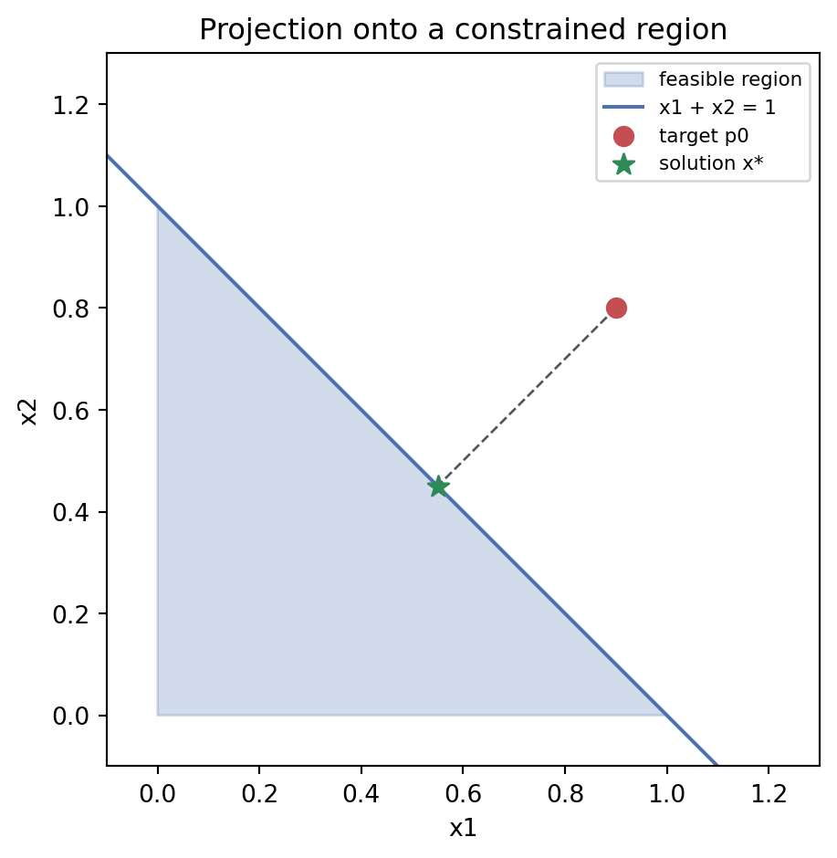
To see complementary slackness pick out the active set, project the point \(p_0 = (0.9, 0.8)\) onto the region \(\{x : x_1 + x_2 \le 1, \ x \ge 0\}\), that is, minimize \(\tfrac{1}{2}\|x - p_0\|^2\) subject to those constraints. Writing \(g_0(x) = x_1 + x_2 - 1\), \(g_1(x) = -x_1\), \(g_2(x) = -x_2\), stationarity reads
Since \(p_0\) lies in the positive orthant but violates the sum constraint, we guess that only \(g_0\) is active: \(\lambda_1 = \lambda_2 = 0\) by complementary slackness. Then \(x = p_0 - \lambda_0 (1,1)\), and enforcing \(x_1 + x_2 = 1\) gives \(\lambda_0 = \tfrac{1}{2}(0.9 + 0.8 - 1) = 0.35 \ge 0\), satisfying dual feasibility. The solution is \(x^\star = (0.55, 0.45)\), which is feasible and confirms the guessed active set. The Python section reproduces this value with a generic solver, showing that the numerical optimizer lands on exactly the active constraint predicted by the KKT analysis.
47.3.6 3.6 Constraint qualifications
The KKT conditions are necessary for optimality only when the constraints are well behaved at \(x^\star\). The mildest common assumption is the linear independence constraint qualification, which requires the gradients of the active inequality constraints and all equality constraints to be linearly independent at \(x^\star\). Another standard one is Slater’s condition for convex problems, which requires a strictly feasible point where every inequality constraint holds with strict inequality. When such a qualification fails, the geometry can become degenerate and a minimizer may not admit valid multipliers. For the convex problems that dominate machine learning, Slater’s condition usually holds and the KKT conditions become both necessary and sufficient for global optimality.
47.4 4. Duality
47.4.1 4.1 The dual function
The Lagrangian gives rise to a second optimization problem that is often easier to solve and always informative. Define the dual function by minimizing the Lagrangian over the primal variable,
Because \(q\) is an infimum of affine functions of \((\lambda, \nu)\), it is concave regardless of whether the original problem is convex. For any feasible \(x\) and any \(\lambda \ge 0\), each term \(\lambda_i g_i(x)\) is nonpositive and each \(\nu_j h_j(x)\) vanishes, so \(q(\lambda, \nu) \le f(x)\). The dual function therefore provides a lower bound on the optimal value for every choice of nonnegative \(\lambda\). The best such bound is found by solving the dual problem
Let \(p^\star\) be the optimal primal value and \(d^\star\) the optimal dual value. Weak duality says \(d^\star \le p^\star\) always. The gap \(p^\star - d^\star\) is the duality gap. For convex problems satisfying a constraint qualification such as Slater’s condition, strong duality holds and the gap closes: \(d^\star = p^\star\). Strong duality is what makes the dual approach practical. It means we may solve whichever of the two problems is more convenient and recover the optimal value of the other. In the support vector machine the dual turns out to expose the structure that makes kernels possible, which is the subject of the next section.
47.5 5. Applications in Machine Learning
47.5.1 5.1 Support vector machines
The support vector machine is the canonical example of constrained optimization in machine learning, and its derivation showcases every tool above. Given labeled data \((x_i, y_i)\) with \(y_i \in \{-1, +1\}\), the hard-margin SVM seeks the hyperplane \(w^\top x + b = 0\) that separates the classes with the widest margin. This is the problem
\[
\begin{aligned}
\min_{w, b} \quad & \tfrac{1}{2} \|w\|^2 \\
\text{subject to} \quad & y_i (w^\top x_i + b) \ge 1, \quad i = 1, \dots, N.
\end{aligned}
\]
Rewriting each constraint as \(1 - y_i(w^\top x_i + b) \le 0\) and introducing multipliers \(\alpha_i \ge 0\) gives the Lagrangian
The first equation is striking. The optimal weight vector is a linear combination of the training inputs, weighted by the multipliers and the labels. Substituting back produces the dual problem
Two consequences follow directly from KKT theory. First, complementary slackness, \(\alpha_i [y_i(w^\top x_i + b) - 1] = 0\), forces \(\alpha_i = 0\) for every point that lies strictly outside the margin. Only points on the margin boundary, where the constraint is active, can have \(\alpha_i > 0\). These are the support vectors, and they alone determine the classifier. The model’s sparsity is a direct expression of complementary slackness. Second, the dual depends on the inputs only through inner products \(x_i^\top x_k\). Replacing these with a kernel \(K(x_i, x_k)\) lets the SVM operate in a high-dimensional feature space without ever forming the features explicitly. The kernel trick is a gift of the dual formulation. The soft-margin variant adds slack variables and an upper bound \(C\) on each \(\alpha_i\), but the structure is identical.
47.5.2 5.2 Maximum entropy models
The principle of maximum entropy says that among all distributions consistent with what we know, we should choose the one with the greatest entropy, since it commits to nothing beyond the given evidence. Concretely, we maximize the entropy \(H(p) = -\sum_x p(x) \log p(x)\) subject to a normalization constraint \(\sum_x p(x) = 1\) and a set of moment constraints \(\sum_x p(x) f_k(x) = \mu_k\) that match observed feature averages.
This is a constrained optimization over a probability vector. Forming the Lagrangian
and setting the derivative with respect to each \(p(x)\) to zero gives \(-\log p(x) - 1 + \nu + \sum_k \lambda_k f_k(x) = 0\). Solving for \(p(x)\) produces the exponential family form
where \(Z\) normalizes the distribution. The multipliers \(\lambda_k\) become the natural parameters of the model. This derivation is the reason logistic regression, softmax classifiers, and conditional random fields all share the same exponential functional form: each is a maximum entropy model under linear feature constraints, and the Lagrange multipliers reappear as learned weights.
47.5.3 5.3 Projected gradient methods
The theory describes optima, but algorithms must reach them. When the feasible set \(\mathcal{C}\) is convex, projected gradient descent offers a clean iterative method. Each step takes an ordinary gradient step and then projects the result back onto the feasible set,
where the projection \(\Pi_{\mathcal{C}}(z) = \arg\min_{x \in \mathcal{C}} \|x - z\|^2\) returns the nearest feasible point. The projection is itself a small constrained optimization, and for common sets it has a closed form. Projecting onto a Euclidean ball rescales the vector to the boundary when it lies outside. Projecting onto the nonnegative orthant clips negative entries to zero. Projecting onto the probability simplex sorts and thresholds the entries.
The connection to KKT theory runs deep. A fixed point of the projected gradient iteration, where \(x^\star = \Pi_{\mathcal{C}}(x^\star - \eta \nabla f(x^\star))\), satisfies the KKT conditions of the constrained problem. The projection operator silently enforces dual feasibility and complementary slackness at each step, which is why the method converges to a genuine constrained optimum rather than an unconstrained one. Projected gradient descent and its proximal generalizations underpin much of constrained and regularized learning, from nonnegative matrix factorization to sparse regression and beyond.
47.6 6. Solving Constrained Problems in Code
The two worked examples above admit a clean computational treatment. The equality-constrained quadratic reduces to a single linear solve through its KKT system, and the inequality-constrained projection is handled by a general-purpose nonlinear solver. The tabset below shows the same workflow in three languages. The Python panel is executable and produces the output and figure inline; the Julia and Rust panels are illustrative and mirror the same logic in their idiomatic numerical ecosystems.
The optimizer lands on \(x^\star = (0.55, 0.45)\), sitting exactly on the line \(x_1 + x_2 = 1\). The zero residual confirms the sum constraint is active, matching the active set the KKT analysis predicted.
usingLinearAlgebra# Equality-constrained quadratic via the KKT linear system# minimize 1/2 x'Qx + c'x subject to A x = bQ = [2.00.0; 0.02.0]c = [0.0, 0.0]A =reshape([1.0, 1.0], 1, 2)b = [1.0]n, p =size(Q, 1), size(A, 1)KKT = [Q A'; A zeros(p, p)]rhs =vcat(-c, b)sol = KKT \ rhsx_eq, nu = sol[1:n], sol[n+1:end]println("Equality-constrained QP: x* = ", x_eq, ", nu* = ", nu)# Inequality-constrained projection via JuMP + Ipopt (illustrative)usingJuMP, Ipoptp0 = [0.9, 0.8]model =Model(Ipopt.Optimizer)@variable(model, x[1:2] >=0)@constraint(model, x[1] + x[2] <=1)@objective(model, Min, 0.5*sum((x .- p0) .^2))optimize!(model)println("Inequality-constrained QP: x* = ", value.(x))
// Equality-constrained quadratic via the KKT linear system.// Solve [[Q, A^T],[A, 0]] [x; nu] = [-c; b] with nalgebra (illustrative).usenalgebra::{DMatrix, DVector};fn main() {let q =DMatrix::from_row_slice(2,2,&[2.0,0.0,0.0,2.0]);let a =DMatrix::from_row_slice(1,2,&[1.0,1.0]);let c =DVector::from_row_slice(&[0.0,0.0]);let b =DVector::from_row_slice(&[1.0]);let (n, p) = (q.nrows(), a.nrows());// Assemble the (n+p) x (n+p) symmetric KKT block matrix.letmut kkt =DMatrix::zeros(n + p, n + p); kkt.view_mut((0,0), (n, n)).copy_from(&q); kkt.view_mut((0, n), (n, p)).copy_from(&a.transpose()); kkt.view_mut((n,0), (p, n)).copy_from(&a);letmut rhs =DVector::zeros(n + p); rhs.rows_mut(0, n).copy_from(&(-&c)); rhs.rows_mut(n, p).copy_from(&b);let sol = kkt.lu().solve(&rhs).expect("KKT system is singular");let x = sol.rows(0, n);let nu = sol.rows(n, p);println!("x* = {:?}, nu* = {:?}", x.as_slice(), nu.as_slice());// Expected: x* = [0.5, 0.5], nu* = [-1.0]}
47.7 7. Summary
Constrained optimization replaces the vanishing-gradient condition of unconstrained problems with a balance of forces between the objective and the constraints. For equality constraints this balance is captured by Lagrange multipliers and the requirement that the objective gradient lie in the span of the constraint gradients. Inequality constraints add the sign condition \(\lambda \ge 0\) and complementary slackness, and the full package becomes the KKT conditions, which are necessary for optimality under a constraint qualification and sufficient for convex problems. Duality turns these conditions into a second problem that bounds and, in the convex case, equals the original. These ideas are not abstractions layered on top of machine learning. They are the machinery that produces support vectors and kernels, that explains why maximum entropy yields exponential family models, and that guarantees projected gradient methods land on the constraint boundary they are meant to respect.
47.8 References
Boyd, S., and Vandenberghe, L. Convex Optimization. Cambridge University Press, 2004. https://doi.org/10.1017/CBO9780511804441
Nocedal, J., and Wright, S. Numerical Optimization, 2nd ed. Springer, 2006. https://doi.org/10.1007/978-0-387-40065-5
Kuhn, H. W., and Tucker, A. W. “Nonlinear Programming.” Proceedings of the Second Berkeley Symposium on Mathematical Statistics and Probability, 1951, pp. 481 to 492. https://projecteuclid.org/euclid.bsmsp/1200500249
Cortes, C., and Vapnik, V. “Support-Vector Networks.” Machine Learning, vol. 20, no. 3, 1995, pp. 273 to 297. https://doi.org/10.1007/BF00994018
Jaynes, E. T. “Information Theory and Statistical Mechanics.” Physical Review, vol. 106, no. 4, 1957, pp. 620 to 630. https://doi.org/10.1103/PhysRev.106.620
Berger, A. L., Della Pietra, S. A., and Della Pietra, V. J. “A Maximum Entropy Approach to Natural Language Processing.” Computational Linguistics, vol. 22, no. 1, 1996, pp. 39 to 71. https://aclanthology.org/J96-1002/
Parikh, N., and Boyd, S. “Proximal Algorithms.” Foundations and Trends in Optimization, vol. 1, no. 3, 2014, pp. 127 to 239. https://doi.org/10.1561/2400000003
Bertsekas, D. P. Nonlinear Programming, 3rd ed. Athena Scientific, 2016. http://www.athenasc.com/nonlinbook.html
Bertsekas, D. P. Constrained Optimization and Lagrange Multiplier Methods. Academic Press, 1982. https://doi.org/10.1016/C2013-0-10366-2
Source Code
# Constrained OptimizationMost optimization problems in machine learning do not ask us to minimize a function over all of space. They ask us to minimize a function subject to restrictions: a probability vector must sum to one, a classifier margin must exceed a threshold, a set of weights must lie inside a ball. Constrained optimization is the mathematical language for these situations, and the theory built around Lagrange multipliers and the Karush-Kuhn-Tucker (KKT) conditions is among the most useful tools a practitioner can carry. This chapter develops that theory from first principles, builds the geometric intuition behind it, and connects it directly to the algorithms that power support vector machines, maximum entropy models, and projected gradient methods.## 1. The Constrained Optimization Problem### 1.1 Standard formA general constrained optimization problem can be written as$$\begin{aligned}\min_{x \in \mathbb{R}^n} \quad & f(x) \\\text{subject to} \quad & g_i(x) \le 0, \quad i = 1, \dots, m, \\& h_j(x) = 0, \quad j = 1, \dots, p.\end{aligned}$$Here $f$ is the objective function, the $g_i$ encode inequality constraints, and the $h_j$ encode equality constraints. The set of points satisfying every constraint is the feasible set,$$\mathcal{F} = \{ x : g_i(x) \le 0 \ \forall i, \ h_j(x) = 0 \ \forall j \}.$$We seek a point in $\mathcal{F}$ that achieves the smallest value of $f$. Maximization problems fold into this form by minimizing $-f$, and a constraint of the form $g_i(x) \ge 0$ becomes $-g_i(x) \le 0$. The convention of writing inequalities as $\le 0$ is not cosmetic. It fixes the sign of the multipliers that appear later, which is exactly where careful bookkeeping pays off.### 1.2 Why unconstrained intuition failsIn unconstrained optimization a minimizer satisfies $\nabla f(x) = 0$: the function is locally flat at an optimum. Constraints break this picture. The minimum of $f(x) = x^2$ over $\mathbb{R}$ sits at $x = 0$, but the minimum subject to $x \ge 1$ sits at $x = 1$, where $\nabla f = 2 \ne 0$. The gradient does not vanish because the boundary of the feasible set blocks any further descent. The function still wants to decrease, but the constraint pushes back with an equal and opposite force. Capturing that balance of forces is the entire content of the theory that follows.## 2. Equality Constraints and Lagrange Multipliers### 2.1 The geometric conditionConsider first the simplest constrained problem, minimizing $f(x)$ subject to a single equality constraint $h(x) = 0$. The constraint defines a surface, and feasible directions are those that stay on the surface. At a point $x$, a direction $v$ keeps us on the surface to first order when $\nabla h(x)^\top v = 0$, that is, when $v$ is tangent to the surface.Suppose $x^\star$ is a local minimizer along this surface. Then $f$ cannot decrease in any feasible direction, so $\nabla f(x^\star)^\top v = 0$ for every tangent direction $v$. This means $\nabla f(x^\star)$ is orthogonal to the tangent space, and the tangent space is exactly the set of vectors orthogonal to $\nabla h(x^\star)$. Two vectors orthogonal to the same hyperplane must be parallel, so there exists a scalar $\lambda$ with$$\nabla f(x^\star) = -\lambda \nabla h(x^\star).$$The scalar $\lambda$ is the Lagrange multiplier. The geometric reading is clean: at an optimum the gradient of the objective is parallel to the gradient of the constraint. If it had any component along the surface, we could slide in that direction and lower $f$.### 2.2 The LagrangianRather than reason about tangent spaces each time, we package the condition into a single function. Define the Lagrangian$$\mathcal{L}(x, \lambda) = f(x) + \lambda h(x).$$Setting its gradient with respect to $x$ to zero recovers $\nabla f + \lambda \nabla h = 0$, and setting its derivative with respect to $\lambda$ to zero recovers the constraint $h(x) = 0$. The stationary points of the Lagrangian are therefore exactly the candidate solutions. With several equality constraints $h_j(x) = 0$ the construction generalizes to$$\mathcal{L}(x, \lambda) = f(x) + \sum_{j=1}^p \lambda_j h_j(x),$$and stationarity in $x$ gives $\nabla f(x^\star) + \sum_j \lambda_j \nabla h_j(x^\star) = 0$. Geometrically the objective gradient is a linear combination of the constraint gradients.### 2.3 A worked example: equality-constrained quadraticThe cleanest setting to see Lagrange multipliers at work is an equality-constrained quadratic, because it admits a closed-form solution that we can verify by hand and then reproduce numerically. Consider the program$$\min_{x \in \mathbb{R}^n} \ \tfrac{1}{2} x^\top Q x + c^\top x \quad \text{subject to} \quad A x = b,$$with $Q$ symmetric positive definite, $A \in \mathbb{R}^{p \times n}$ of full row rank, and $b \in \mathbb{R}^p$. The Lagrangian is$$\mathcal{L}(x, \nu) = \tfrac{1}{2} x^\top Q x + c^\top x + \nu^\top (A x - b).$$Stationarity in $x$ gives $Q x + c + A^\top \nu = 0$, and the constraint gives $A x = b$. Stacking the two conditions produces the symmetric KKT system$$\begin{bmatrix} Q & A^\top \\ A & 0 \end{bmatrix}\begin{bmatrix} x^\star \\ \nu^\star \end{bmatrix}=\begin{bmatrix} -c \\ b \end{bmatrix},$$a single linear solve. Because $Q \succ 0$ and $A$ has full row rank, the block matrix is invertible and the solution is unique. Specializing to $f(x_1, x_2) = x_1^2 + x_2^2$ subject to $x_1 + x_2 = 1$ we have $Q = 2 I$, $c = 0$, $A = [1 \ 1]$, $b = 1$. Stationarity gives $2x_1 + \nu = 0$ and $2x_2 + \nu = 0$, so $x_1 = x_2 = -\nu/2$. The constraint forces $-\nu = 1$, hence $x_1 = x_2 = 1/2$ with $\nu = -1$. The closest point on the line to the origin is its midpoint, which matches intuition. The multiplier value $\nu = -1$ also carries meaning, which the next subsection makes precise. The Python section below assembles and solves this exact KKT system.### 2.4 Sensitivity interpretationSuppose we perturb the constraint to $h(x) = c$ and let $p^\star(c)$ be the resulting optimal value. A standard result states that$$\frac{d p^\star}{d c} = -\lambda^\star.$$The multiplier measures how sensitive the optimum is to relaxing the constraint. In economics this is the shadow price: the marginal value of one more unit of a resource. In machine learning the same idea explains why multipliers carry units that relate the objective to the constraint, and why a large multiplier flags a constraint that is binding hard against the objective.## 3. Inequality Constraints and the KKT Conditions### 3.1 Active and inactive constraintsInequality constraints introduce a qualitative twist. An inequality $g_i(x) \le 0$ is either active at $x^\star$, meaning $g_i(x^\star) = 0$ and the point sits on that boundary, or inactive, meaning $g_i(x^\star) < 0$ and the point lies strictly inside. An inactive constraint exerts no force at the optimum. If we are strictly inside the feasible region with room to spare, that constraint plays no role in the local balance and behaves as if it were absent. An active constraint behaves like an equality constraint, since the optimum is pinned to its boundary.The difficulty is that we usually do not know in advance which constraints will be active. The KKT conditions resolve this by encoding the active or inactive distinction algebraically through a sign condition and a complementarity condition.### 3.2 The KKT conditionsFor the general problem of Section 1.1, define the full Lagrangian$$\mathcal{L}(x, \lambda, \nu) = f(x) + \sum_{i=1}^m \lambda_i g_i(x) + \sum_{j=1}^p \nu_j h_j(x),$$with multipliers $\lambda_i$ for inequalities and $\nu_j$ for equalities. Under a suitable regularity assumption discussed below, if $x^\star$ is a local minimizer then there exist multipliers $\lambda^\star$ and $\nu^\star$ such that the following hold.Stationarity:$$\nabla f(x^\star) + \sum_{i=1}^m \lambda_i^\star \nabla g_i(x^\star) + \sum_{j=1}^p \nu_j^\star \nabla h_j(x^\star) = 0.$$Primal feasibility:$$g_i(x^\star) \le 0, \qquad h_j(x^\star) = 0.$$Dual feasibility:$$\lambda_i^\star \ge 0.$$Complementary slackness:$$\lambda_i^\star \, g_i(x^\star) = 0 \quad \text{for all } i.$$These four groups are the KKT conditions. The stationarity condition is the force balance generalized to many constraints. Primal feasibility simply says the solution obeys the constraints. The two conditions that deserve close attention are dual feasibility and complementary slackness.### 3.3 Why the multipliers must be nonnegativeFor an inequality $g_i(x) \le 0$, feasibility lies in the direction where $g_i$ decreases. At an active constraint the objective gradient must point in a direction that the constraint forbids, otherwise we could step into the feasible interior and lower $f$. Writing the force balance for a single active constraint, $\nabla f = -\lambda \nabla g$, the multiplier must be nonnegative so that the objective gradient and the inward-pointing constraint force oppose each other. If $\lambda$ were negative the objective could decrease by moving into the feasible region, contradicting optimality. This sign asymmetry is the crucial difference from equality constraints, whose multipliers are free in sign because an equality blocks motion in both directions.### 3.4 Complementary slacknessComplementary slackness states that for each $i$, at least one of $\lambda_i^\star$ and $g_i(x^\star)$ is zero. The two cases correspond exactly to the active and inactive distinction. If a constraint is inactive, $g_i(x^\star) < 0$, then $\lambda_i^\star = 0$ and the constraint drops out of the stationarity equation, just as intuition demands for a constraint with slack. If a multiplier is strictly positive, $\lambda_i^\star > 0$, then $g_i(x^\star) = 0$ and the constraint is active, contributing a genuine force. Complementary slackness is what lets a single set of equations describe a solution without knowing the active set ahead of time. Solving the KKT system amounts to finding the right active set such that all four conditions hold simultaneously.### 3.5 A worked KKT exampleTo see complementary slackness pick out the active set, project the point $p_0 = (0.9, 0.8)$ onto the region $\{x : x_1 + x_2 \le 1, \ x \ge 0\}$, that is, minimize $\tfrac{1}{2}\|x - p_0\|^2$ subject to those constraints. Writing $g_0(x) = x_1 + x_2 - 1$, $g_1(x) = -x_1$, $g_2(x) = -x_2$, stationarity reads$$(x - p_0) + \lambda_0 \begin{bmatrix} 1 \\ 1 \end{bmatrix} - \lambda_1 \begin{bmatrix} 1 \\ 0 \end{bmatrix} - \lambda_2 \begin{bmatrix} 0 \\ 1 \end{bmatrix} = 0.$$Since $p_0$ lies in the positive orthant but violates the sum constraint, we guess that only $g_0$ is active: $\lambda_1 = \lambda_2 = 0$ by complementary slackness. Then $x = p_0 - \lambda_0 (1,1)$, and enforcing $x_1 + x_2 = 1$ gives $\lambda_0 = \tfrac{1}{2}(0.9 + 0.8 - 1) = 0.35 \ge 0$, satisfying dual feasibility. The solution is $x^\star = (0.55, 0.45)$, which is feasible and confirms the guessed active set. The Python section reproduces this value with a generic solver, showing that the numerical optimizer lands on exactly the active constraint predicted by the KKT analysis.### 3.6 Constraint qualificationsThe KKT conditions are necessary for optimality only when the constraints are well behaved at $x^\star$. The mildest common assumption is the linear independence constraint qualification, which requires the gradients of the active inequality constraints and all equality constraints to be linearly independent at $x^\star$. Another standard one is Slater's condition for convex problems, which requires a strictly feasible point where every inequality constraint holds with strict inequality. When such a qualification fails, the geometry can become degenerate and a minimizer may not admit valid multipliers. For the convex problems that dominate machine learning, Slater's condition usually holds and the KKT conditions become both necessary and sufficient for global optimality.## 4. Duality### 4.1 The dual functionThe Lagrangian gives rise to a second optimization problem that is often easier to solve and always informative. Define the dual function by minimizing the Lagrangian over the primal variable,$$q(\lambda, \nu) = \inf_{x} \ \mathcal{L}(x, \lambda, \nu).$$Because $q$ is an infimum of affine functions of $(\lambda, \nu)$, it is concave regardless of whether the original problem is convex. For any feasible $x$ and any $\lambda \ge 0$, each term $\lambda_i g_i(x)$ is nonpositive and each $\nu_j h_j(x)$ vanishes, so $q(\lambda, \nu) \le f(x)$. The dual function therefore provides a lower bound on the optimal value for every choice of nonnegative $\lambda$. The best such bound is found by solving the dual problem$$\max_{\lambda \ge 0, \, \nu} \ q(\lambda, \nu).$$### 4.2 Weak and strong dualityLet $p^\star$ be the optimal primal value and $d^\star$ the optimal dual value. Weak duality says $d^\star \le p^\star$ always. The gap $p^\star - d^\star$ is the duality gap. For convex problems satisfying a constraint qualification such as Slater's condition, strong duality holds and the gap closes: $d^\star = p^\star$. Strong duality is what makes the dual approach practical. It means we may solve whichever of the two problems is more convenient and recover the optimal value of the other. In the support vector machine the dual turns out to expose the structure that makes kernels possible, which is the subject of the next section.## 5. Applications in Machine Learning### 5.1 Support vector machinesThe support vector machine is the canonical example of constrained optimization in machine learning, and its derivation showcases every tool above. Given labeled data $(x_i, y_i)$ with $y_i \in \{-1, +1\}$, the hard-margin SVM seeks the hyperplane $w^\top x + b = 0$ that separates the classes with the widest margin. This is the problem$$\begin{aligned}\min_{w, b} \quad & \tfrac{1}{2} \|w\|^2 \\\text{subject to} \quad & y_i (w^\top x_i + b) \ge 1, \quad i = 1, \dots, N.\end{aligned}$$Rewriting each constraint as $1 - y_i(w^\top x_i + b) \le 0$ and introducing multipliers $\alpha_i \ge 0$ gives the Lagrangian$$\mathcal{L}(w, b, \alpha) = \tfrac{1}{2}\|w\|^2 - \sum_{i=1}^N \alpha_i \big( y_i (w^\top x_i + b) - 1 \big).$$Stationarity with respect to $w$ and $b$ yields$$w = \sum_{i=1}^N \alpha_i y_i x_i, \qquad \sum_{i=1}^N \alpha_i y_i = 0.$$The first equation is striking. The optimal weight vector is a linear combination of the training inputs, weighted by the multipliers and the labels. Substituting back produces the dual problem$$\begin{aligned}\max_{\alpha} \quad & \sum_{i=1}^N \alpha_i - \tfrac{1}{2} \sum_{i=1}^N \sum_{k=1}^N \alpha_i \alpha_k y_i y_k \, x_i^\top x_k \\\text{subject to} \quad & \alpha_i \ge 0, \quad \sum_{i=1}^N \alpha_i y_i = 0.\end{aligned}$$Two consequences follow directly from KKT theory. First, complementary slackness, $\alpha_i [y_i(w^\top x_i + b) - 1] = 0$, forces $\alpha_i = 0$ for every point that lies strictly outside the margin. Only points on the margin boundary, where the constraint is active, can have $\alpha_i > 0$. These are the support vectors, and they alone determine the classifier. The model's sparsity is a direct expression of complementary slackness. Second, the dual depends on the inputs only through inner products $x_i^\top x_k$. Replacing these with a kernel $K(x_i, x_k)$ lets the SVM operate in a high-dimensional feature space without ever forming the features explicitly. The kernel trick is a gift of the dual formulation. The soft-margin variant adds slack variables and an upper bound $C$ on each $\alpha_i$, but the structure is identical.### 5.2 Maximum entropy modelsThe principle of maximum entropy says that among all distributions consistent with what we know, we should choose the one with the greatest entropy, since it commits to nothing beyond the given evidence. Concretely, we maximize the entropy $H(p) = -\sum_x p(x) \log p(x)$ subject to a normalization constraint $\sum_x p(x) = 1$ and a set of moment constraints $\sum_x p(x) f_k(x) = \mu_k$ that match observed feature averages.This is a constrained optimization over a probability vector. Forming the Lagrangian$$\mathcal{L} = -\sum_x p(x) \log p(x) + \nu \Big( \sum_x p(x) - 1 \Big) + \sum_k \lambda_k \Big( \sum_x p(x) f_k(x) - \mu_k \Big),$$and setting the derivative with respect to each $p(x)$ to zero gives $-\log p(x) - 1 + \nu + \sum_k \lambda_k f_k(x) = 0$. Solving for $p(x)$ produces the exponential family form$$p(x) = \frac{1}{Z} \exp\Big( \sum_k \lambda_k f_k(x) \Big),$$where $Z$ normalizes the distribution. The multipliers $\lambda_k$ become the natural parameters of the model. This derivation is the reason logistic regression, softmax classifiers, and conditional random fields all share the same exponential functional form: each is a maximum entropy model under linear feature constraints, and the Lagrange multipliers reappear as learned weights.### 5.3 Projected gradient methodsThe theory describes optima, but algorithms must reach them. When the feasible set $\mathcal{C}$ is convex, projected gradient descent offers a clean iterative method. Each step takes an ordinary gradient step and then projects the result back onto the feasible set,$$x_{t+1} = \Pi_{\mathcal{C}} \big( x_t - \eta \nabla f(x_t) \big),$$where the projection $\Pi_{\mathcal{C}}(z) = \arg\min_{x \in \mathcal{C}} \|x - z\|^2$ returns the nearest feasible point. The projection is itself a small constrained optimization, and for common sets it has a closed form. Projecting onto a Euclidean ball rescales the vector to the boundary when it lies outside. Projecting onto the nonnegative orthant clips negative entries to zero. Projecting onto the probability simplex sorts and thresholds the entries.The connection to KKT theory runs deep. A fixed point of the projected gradient iteration, where $x^\star = \Pi_{\mathcal{C}}(x^\star - \eta \nabla f(x^\star))$, satisfies the KKT conditions of the constrained problem. The projection operator silently enforces dual feasibility and complementary slackness at each step, which is why the method converges to a genuine constrained optimum rather than an unconstrained one. Projected gradient descent and its proximal generalizations underpin much of constrained and regularized learning, from nonnegative matrix factorization to sparse regression and beyond.## 6. Solving Constrained Problems in CodeThe two worked examples above admit a clean computational treatment. The equality-constrained quadratic reduces to a single linear solve through its KKT system, and the inequality-constrained projection is handled by a general-purpose nonlinear solver. The tabset below shows the same workflow in three languages. The Python panel is executable and produces the output and figure inline; the Julia and Rust panels are illustrative and mirror the same logic in their idiomatic numerical ecosystems.::: {.panel-tabset}## Python```{python}import numpy as npfrom scipy.optimize import minimizeimport matplotlib.pyplot as pltnp.random.seed(42)# Part 1: equality-constrained quadratic solved via the KKT linear system# minimize 1/2 x^T Q x + c^T x subject to A x = bQ = np.array([[2.0, 0.0], [0.0, 2.0]])c = np.array([0.0, 0.0])A = np.array([[1.0, 1.0]])b = np.array([1.0])n, p = Q.shape[0], A.shape[0]KKT = np.block([[Q, A.T], [A, np.zeros((p, p))]])rhs = np.concatenate([-c, b])sol = np.linalg.solve(KKT, rhs)x_eq, nu = sol[:n], sol[n:]print(f"Equality-constrained QP: x* = {x_eq}, nu* = {nu}")# Part 2: inequality-constrained projection solved with scipy SLSQP# minimize 1/2 ||x - p0||^2 subject to x1 + x2 <= 1, x >= 0p0 = np.array([0.9, 0.8])obj =lambda x: 0.5* np.sum((x - p0) **2)grad =lambda x: x - p0cons = [{"type": "ineq", "fun": lambda x: 1.0- (x[0] + x[1])}]bnds = [(0.0, None), (0.0, None)]res = minimize(obj, np.zeros(2), jac=grad, bounds=bnds, constraints=cons, method="SLSQP")print(f"Inequality-constrained QP: x* = {res.x}, objective = {res.fun:.4f}")print(f"Active set residual (x1+x2-1) = {res.x[0] + res.x[1] -1:.6f}")# Visualize the feasible region and the solutionfig, ax = plt.subplots(figsize=(5.5, 5.0))ax.fill([0, 1, 0], [0, 0, 1], alpha=0.25, color="#4C72B0", label="feasible region")xs = np.linspace(-0.1, 1.3, 100)ax.plot(xs, 1- xs, color="#4C72B0", lw=1.5, label="x1 + x2 = 1")ax.scatter(*p0, color="#C44E52", s=60, zorder=5, label="target p0")ax.scatter(*res.x, color="#2E8B57", s=80, marker="*", zorder=5, label="solution x*")ax.plot([p0[0], res.x[0]], [p0[1], res.x[1]], "--", color="#555555", lw=1.0)ax.set_xlim(-0.1, 1.3); ax.set_ylim(-0.1, 1.3)ax.set_xlabel("x1"); ax.set_ylabel("x2")ax.set_title("Projection onto a constrained region")ax.legend(loc="upper right", fontsize=8); ax.set_aspect("equal")plt.tight_layout()plt.show()```The optimizer lands on $x^\star = (0.55, 0.45)$, sitting exactly on the line $x_1 + x_2 = 1$. The zero residual confirms the sum constraint is active, matching the active set the KKT analysis predicted.## Julia```juliausingLinearAlgebra# Equality-constrained quadratic via the KKT linear system# minimize 1/2 x'Qx + c'x subject to A x = bQ = [2.00.0; 0.02.0]c = [0.0, 0.0]A =reshape([1.0, 1.0], 1, 2)b = [1.0]n, p =size(Q, 1), size(A, 1)KKT = [Q A'; A zeros(p, p)]rhs =vcat(-c, b)sol = KKT \ rhsx_eq, nu = sol[1:n], sol[n+1:end]println("Equality-constrained QP: x* = ", x_eq, ", nu* = ", nu)# Inequality-constrained projection via JuMP + Ipopt (illustrative)usingJuMP, Ipoptp0 = [0.9, 0.8]model =Model(Ipopt.Optimizer)@variable(model, x[1:2] >=0)@constraint(model, x[1] + x[2] <=1)@objective(model, Min, 0.5*sum((x .- p0) .^2))optimize!(model)println("Inequality-constrained QP: x* = ", value.(x))```## Rust```rust// Equality-constrained quadratic via the KKT linear system.// Solve [[Q, A^T],[A, 0]] [x; nu] = [-c; b] with nalgebra (illustrative).use nalgebra::{DMatrix, DVector};fn main() { let q = DMatrix::from_row_slice(2, 2, &[2.0, 0.0, 0.0, 2.0]); let a = DMatrix::from_row_slice(1, 2, &[1.0, 1.0]); let c = DVector::from_row_slice(&[0.0, 0.0]); let b = DVector::from_row_slice(&[1.0]);let (n, p) = (q.nrows(), a.nrows());// Assemble the (n+p) x (n+p) symmetric KKT block matrix. let mut kkt = DMatrix::zeros(n + p, n + p);kkt.view_mut((0, 0), (n, n)).copy_from(&q);kkt.view_mut((0, n), (n, p)).copy_from(&a.transpose());kkt.view_mut((n, 0), (p, n)).copy_from(&a); let mut rhs = DVector::zeros(n + p);rhs.rows_mut(0, n).copy_from(&(-&c));rhs.rows_mut(n, p).copy_from(&b); let sol =kkt.lu().solve(&rhs).expect("KKT system is singular"); let x =sol.rows(0, n); let nu =sol.rows(n, p); println!("x* = {:?}, nu* = {:?}", x.as_slice(), nu.as_slice());// Expected: x*= [0.5, 0.5], nu*= [-1.0]}```:::## 7. SummaryConstrained optimization replaces the vanishing-gradient condition of unconstrained problems with a balance of forces between the objective and the constraints. For equality constraints this balance is captured by Lagrange multipliers and the requirement that the objective gradient lie in the span of the constraint gradients. Inequality constraints add the sign condition $\lambda \ge 0$ and complementary slackness, and the full package becomes the KKT conditions, which are necessary for optimality under a constraint qualification and sufficient for convex problems. Duality turns these conditions into a second problem that bounds and, in the convex case, equals the original. These ideas are not abstractions layered on top of machine learning. They are the machinery that produces support vectors and kernels, that explains why maximum entropy yields exponential family models, and that guarantees projected gradient methods land on the constraint boundary they are meant to respect.## References1. Boyd, S., and Vandenberghe, L. *Convex Optimization*. Cambridge University Press, 2004. https://doi.org/10.1017/CBO97805118044412. Nocedal, J., and Wright, S. *Numerical Optimization*, 2nd ed. Springer, 2006. https://doi.org/10.1007/978-0-387-40065-53. Kuhn, H. W., and Tucker, A. W. "Nonlinear Programming." *Proceedings of the Second Berkeley Symposium on Mathematical Statistics and Probability*, 1951, pp. 481 to 492. https://projecteuclid.org/euclid.bsmsp/12005002494. Cortes, C., and Vapnik, V. "Support-Vector Networks." *Machine Learning*, vol. 20, no. 3, 1995, pp. 273 to 297. https://doi.org/10.1007/BF009940185. Jaynes, E. T. "Information Theory and Statistical Mechanics." *Physical Review*, vol. 106, no. 4, 1957, pp. 620 to 630. https://doi.org/10.1103/PhysRev.106.6206. Berger, A. L., Della Pietra, S. A., and Della Pietra, V. J. "A Maximum Entropy Approach to Natural Language Processing." *Computational Linguistics*, vol. 22, no. 1, 1996, pp. 39 to 71. https://aclanthology.org/J96-1002/7. Parikh, N., and Boyd, S. "Proximal Algorithms." *Foundations and Trends in Optimization*, vol. 1, no. 3, 2014, pp. 127 to 239. https://doi.org/10.1561/24000000038. Bertsekas, D. P. *Nonlinear Programming*, 3rd ed. Athena Scientific, 2016. http://www.athenasc.com/nonlinbook.html9. Bertsekas, D. P. *Constrained Optimization and Lagrange Multiplier Methods*. Academic Press, 1982. https://doi.org/10.1016/C2013-0-10366-2