flowchart LR
    A[Regularized objective] --> B[Second-order Taylor expansion]
    B --> C[Optimal leaf weight w*]
    C --> D[Structure score]
    D --> E[Split gain criterion]
    E --> F[Greedy tree growth]
    F --> G[Shrinkage by eta]
    G --> H{More rounds?}
    H -->|yes| B
    H -->|no| I[Final ensemble]
112 XGBoost Theory and Practice
XGBoost is one of the most consequential machine learning systems of the past decade. On tabular data, gradient boosted decision trees remain the default choice for practitioners who want strong accuracy without the engineering burden of deep networks, and XGBoost is the implementation that turned the underlying algorithm into a production grade tool. Its dominance in competitions and industry was not an accident of marketing. The library combines a principled regularized objective, a clean second-order optimization view, an exact and approximate split-finding algorithm, native handling of sparsity and missing values, and a system design tuned for cache efficiency and parallelism. This chapter develops each of these pieces from first principles and then turns to the practical question every user eventually faces, which is how to tune the thing.
XGBoost is open source under the Apache 2.0 license, maintained by the Distributed Machine Learning Community, and installable from PyPI with pip install xgboost or imported directly as import xgboost. Everything in this chapter runs against that open-source library, and the worked example below trains a real open-source XGBoost model end to end.
112.1 1. From Additive Models to a Regularized Objective
112.1.1 1.1 The additive ensemble
Gradient boosting builds a predictor as a sum of \(K\) regression trees. For an input \(\mathbf{x}_i\) the prediction is
\[ \hat{y}_i = \sum_{k=1}^{K} f_k(\mathbf{x}_i), \qquad f_k \in \mathcal{F}, \]
where \(\mathcal{F}\) is the space of regression trees. Each tree \(f_k\) maps an input to a real valued score through a piecewise constant function. Concretely a tree has a structure \(q\) that assigns each input to one of \(T\) leaves, and a leaf weight vector \(\mathbf{w} \in \mathbb{R}^T\), so that \(f(\mathbf{x}) = w_{q(\mathbf{x})}\). Importantly these are regression trees even when the task is classification, because the leaf outputs are continuous scores that get combined and then passed through a link function such as the logistic sigmoid.
The ensemble is grown in stages. We do not optimize all \(K\) trees jointly. Instead at iteration \(t\) we hold the existing trees fixed and add one new tree that improves the objective. This stagewise structure is what makes boosting tractable and is the reason the second-order view below is so useful.
112.1.2 1.2 The regularized learning objective
The defining contribution of the XGBoost formulation is to write the objective with an explicit regularization term on tree complexity:
\[ \mathcal{L} = \sum_{i=1}^{n} \ell(y_i, \hat{y}_i) + \sum_{k=1}^{K} \Omega(f_k), \qquad \Omega(f) = \gamma T + \tfrac{1}{2}\lambda \lVert \mathbf{w} \rVert^2 . \]
Here \(\ell\) is any twice differentiable convex loss, \(T\) is the number of leaves in a tree, and \(\mathbf{w}\) is its vector of leaf weights. The hyperparameter \(\gamma\) penalizes the number of leaves, which acts as a complexity cost that a candidate split must overcome before it is accepted. The hyperparameter \(\lambda\) is an \(L^2\) penalty on leaf weights that shrinks scores toward zero and stabilizes the solution. This is the same idea as ridge regularization applied at the level of leaf outputs.
The point of building regularization directly into the objective is that the tree learning procedure then optimizes a quantity that already trades off fit against complexity. Many earlier boosting descriptions added pruning or shrinkage as ad hoc post-processing. By contrast XGBoost derives its split criterion and its leaf weights from a single regularized objective, which is both cleaner and easier to reason about.
112.2 2. The Second-Order (Newton) Approximation
112.2.1 2.1 Taylor expansion of the stagewise loss
At iteration \(t\) the prediction for example \(i\) is \(\hat{y}_i^{(t)} = \hat{y}_i^{(t-1)} + f_t(\mathbf{x}_i)\). Substituting into the objective and keeping only the term for the new tree gives
\[ \mathcal{L}^{(t)} = \sum_{i=1}^{n} \ell\!\left(y_i, \hat{y}_i^{(t-1)} + f_t(\mathbf{x}_i)\right) + \Omega(f_t). \]
Because \(f_t(\mathbf{x}_i)\) is a small correction, we expand the loss to second order in that correction using a Taylor series. Define the gradient and Hessian of the loss with respect to the current prediction,
\[ g_i = \frac{\partial \ell(y_i, \hat{y}^{(t-1)}_i)}{\partial \hat{y}^{(t-1)}_i}, \qquad h_i = \frac{\partial^2 \ell(y_i, \hat{y}^{(t-1)}_i)}{\partial (\hat{y}^{(t-1)}_i)^2}. \]
The second-order approximation of the objective, after dropping the constant loss term that does not depend on \(f_t\), is
\[ \tilde{\mathcal{L}}^{(t)} = \sum_{i=1}^{n} \left[ g_i f_t(\mathbf{x}_i) + \tfrac{1}{2} h_i f_t(\mathbf{x}_i)^2 \right] + \Omega(f_t). \]
This is the heart of the method. Whereas classical gradient boosting fits each tree to the negative gradient with a least squares step, XGBoost uses both the gradient and the curvature. Using the Hessian is exactly a Newton step in function space, and it is the reason the leaf weights and the split gain below have such clean closed forms. For squared error loss the Hessian is constant and the two views coincide, but for losses such as logistic loss the curvature carries real information and the second-order step converges faster and more stably.
112.2.2 2.2 Optimal leaf weights and the structure score
Fix a tree structure \(q\) and let \(I_j = \{ i : q(\mathbf{x}_i) = j \}\) be the set of examples routed to leaf \(j\). Because every example in a leaf receives the same weight \(w_j\), the objective decomposes leaf by leaf:
\[ \tilde{\mathcal{L}}^{(t)} = \sum_{j=1}^{T} \left[ \left(\sum_{i \in I_j} g_i\right) w_j + \tfrac{1}{2}\left(\sum_{i \in I_j} h_i + \lambda\right) w_j^2 \right] + \gamma T . \]
Writing \(G_j = \sum_{i \in I_j} g_i\) and \(H_j = \sum_{i \in I_j} h_i\), each leaf contributes a one dimensional quadratic in \(w_j\),
\[ \tilde{\mathcal{L}}_j(w_j) = G_j\, w_j + \tfrac{1}{2}\,(H_j + \lambda)\, w_j^2 . \]
This is a strictly convex parabola whenever \(H_j + \lambda > 0\), so its unique minimizer is found by setting the derivative to zero,
\[ \frac{\partial \tilde{\mathcal{L}}_j}{\partial w_j} = G_j + (H_j + \lambda)\, w_j = 0 \quad\Longrightarrow\quad w_j^{\star} = -\frac{G_j}{H_j + \lambda}. \]
The second derivative is \(H_j + \lambda > 0\), confirming the stationary point is a minimum. Substituting \(w_j^\star\) back into \(\tilde{\mathcal{L}}_j\) gives the minimal per-leaf value \(-\tfrac{1}{2}\,G_j^2 / (H_j + \lambda)\), and summing over leaves gives the objective value attained by this structure,
\[ \tilde{\mathcal{L}}^{(t)}(q) = -\frac{1}{2}\sum_{j=1}^{T} \frac{G_j^2}{H_j + \lambda} + \gamma T . \]
This quantity is the structure score. It measures how good a fixed tree shape is, lower being better, and it is the objective that the split-finding algorithm greedily improves. Notice how \(\lambda\) enters the denominator to damp leaf weights when the aggregated curvature is small, and how \(\gamma T\) charges a fixed cost per leaf.
112.3 3. Split Finding
112.3.1 3.1 The gain of a candidate split
We cannot enumerate all tree structures, so XGBoost grows trees greedily. Starting from a single leaf, it repeatedly considers splitting a leaf into a left child and a right child. Suppose a leaf with instance set \(I\) is split into \(I_L\) and \(I_R\). Using the structure score, the reduction in objective from this split is
\[ \text{Gain} = \tfrac{1}{2}\left[ \frac{G_L^2}{H_L + \lambda} + \frac{G_R^2}{H_R + \lambda} - \frac{(G_L + G_R)^2}{H_L + H_R + \lambda} \right] - \gamma . \]
The three terms inside the bracket are the score of the left child, the score of the right child, and the score of the parent leaf before splitting. To see where this comes from, recall the structure score contributes \(-\tfrac{1}{2}\,G^2/(H+\lambda)\) per leaf. Splitting replaces the single parent term with two child terms, so the change in objective is
\[ \Delta \tilde{\mathcal{L}} = \underbrace{\left(-\tfrac{1}{2}\tfrac{G_L^2}{H_L+\lambda}\right) + \left(-\tfrac{1}{2}\tfrac{G_R^2}{H_R+\lambda}\right)}_{\text{after split}} - \underbrace{\left(-\tfrac{1}{2}\tfrac{(G_L+G_R)^2}{H_L+H_R+\lambda}\right)}_{\text{before split}} + \gamma . \]
The gain is the negation \(-\Delta\tilde{\mathcal{L}}\), the reduction in objective, which gives the formula above. The trailing \(\gamma\) is the complexity cost of adding one more leaf. A split is worth making only when its gain is positive, which means the improvement in fit must exceed \(\gamma\). This is regularization acting as a built-in pre-pruning rule, and tuning \(\gamma\) directly controls how aggressively the algorithm grows trees.
flowchart TD
    P["Parent leaf I"]
    P -->|"feature m, threshold t"| L["Left child I_L"]
    P -->|"x at m greater than t"| R["Right child I_R"]
    L --> G["Gain equals half of left plus right minus parent, minus gamma"]
    R --> G
    G -->|"Gain greater than 0"| K["Keep split"]
    G -->|"Gain at most 0"| X["Prune"]
| Node | Detail |
|---|---|
| Parent leaf I | \(G = G_L + G_R\), \(H = H_L + H_R\) |
| Left child I_L | score \(G_L^2 / (H_L + \lambda)\) |
| Right child I_R | score \(G_R^2 / (H_R + \lambda)\) |
112.3.2 3.2 The exact greedy algorithm
To find the best split at a leaf, the exact algorithm sorts the instances by each feature value and scans the sorted order, maintaining running sums \(G_L\) and \(H_L\) for everything to the left of the current threshold. Because the parent sums \(G = G_L + G_R\) and \(H = H_L + H_R\) are known, the right side sums follow by subtraction, and the gain at each candidate threshold is computed in constant time. The procedure is summarized below.
for each feature m:
    sort instances in the leaf by feature value x[m]
    G_L = 0, H_L = 0
    for each instance i in sorted order:
        G_L += g_i, H_L += h_i
        G_R = G - G_L, H_R = H - H_L
        gain = 0.5 * (G_L^2/(H_L+lambda) + G_R^2/(H_R+lambda)
                      - G^2/(H+lambda))
        track best (feature, threshold) by gain
The exact algorithm finds the optimal split for the current leaf with respect to the structure score. Its cost is dominated by sorting, which XGBoost amortizes by storing each feature column in a sorted, compressed block so that the sort happens once rather than at every node.
112.3.3 3.3 The approximate and histogram algorithms
Exact split finding requires every feature value to be a candidate threshold, which becomes expensive when the data do not fit in memory or when the number of distinct values is large. The approximate algorithm proposes a smaller set of candidate split points per feature, typically derived from quantiles of the feature distribution, and then aggregates gradient and Hessian statistics into the resulting buckets. Splits are evaluated only at bucket boundaries.
XGBoost uses a weighted quantile sketch to choose these candidates. The novelty is that the quantiles are weighted by the Hessian \(h_i\) rather than by raw instance counts. The justification follows from rewriting the second-order objective as a weighted squared error,
\[ \sum_i \tfrac{1}{2} h_i \left( f_t(\mathbf{x}_i) + \tfrac{g_i}{h_i} \right)^2 + \text{const}, \]
which shows that each instance carries importance proportional to \(h_i\). Placing candidate thresholds at equal weighted mass means that buckets contain roughly equal curvature, which is what the objective actually cares about. The proposal can be done once at the start of training, called the global variant, or refreshed at every node, called the local variant, with the local variant needing fewer candidates per level for the same accuracy.
The modern default in XGBoost is the histogram method, enabled with tree_method="hist". It bins each feature into a fixed number of integer buckets once, then builds per-node histograms of summed gradients and Hessians over those bins. Split finding scans bins rather than raw values, which is fast and cache friendly, and a child histogram can be obtained by subtracting a sibling histogram from the parent, so only the smaller child needs to be built explicitly. This histogram subtraction trick is a major source of speed. The same binned structure is what enables GPU training and underlies the close performance relationship between XGBoost and LightGBM.
112.4 4. Sparsity-Aware Split Finding
112.4.1 4.1 The default direction
Real tabular data is full of missing values, one-hot encoded zeros, and other sources of sparsity. XGBoost treats all of these uniformly through a sparsity-aware split-finding rule. For every split, the algorithm learns a default direction. Instances whose value for the split feature is present are routed normally by comparing against the threshold. Instances whose value is missing, or absent in the sparse representation, are sent to the default branch.
The default direction is not guessed. During split finding the algorithm tries assigning all missing instances to the left child and computes the resulting gain, then tries assigning them all to the right child and computes that gain, and keeps whichever direction yields the higher gain. In effect the optimal handling of missing data is learned from the gradient statistics at each split, rather than being imputed beforehand.
112.4.2 4.2 Why this matters in practice
The mechanism has two consequences worth emphasizing. First, you generally should not impute missing values before handing data to XGBoost, because the model can extract signal from the missingness pattern itself, and a missing value sometimes carries information that an imputed mean would destroy. Second, the algorithm only iterates over the present entries when evaluating splits, so the complexity scales with the number of non-missing values rather than the dense size of the matrix. On sparse inputs this delivers a large speedup, and the original paper reported order of magnitude gains on sparse datasets from this design alone. The same code path handles explicit missing markers and structural zeros, which is why one-hot encoded categorical features train efficiently.
112.5 5. Shrinkage and Column Subsampling
112.5.1 5.1 Shrinkage
The closed-form leaf weight \(w_j^\star\) is the Newton-optimal step for the current round, but taking the full step every round tends to overfit. Shrinkage, introduced by Friedman, scales each new tree by a learning rate \(\eta \in (0, 1]\) before adding it to the ensemble. The update becomes
\[ \hat{y}_i^{(t)} = \hat{y}_i^{(t-1)} + \eta\, f_t(\mathbf{x}_i), \qquad f_t(\mathbf{x}_i) = w_{q(\mathbf{x}_i)}^{\star} . \]
Equivalently each leaf weight is damped to \(\eta\, w_j^\star\). The effect is to take many small steps rather than a few large ones, which leaves room for later trees to correct earlier ones and reduces the variance contributed by any single tree. There is a direct tradeoff with the number of rounds: halving \(\eta\) roughly doubles the rounds \(K\) needed to reach the same training fit, since the cumulative contribution after \(K\) rounds scales like \(\eta K\). In practice you fix a small \(\eta\) and let early stopping choose \(K\).
112.5.2 5.2 Column subsampling
Column subsampling draws, before growing a tree, a random subset \(S \subseteq \{1, \dots, p\}\) of the \(p\) features of size \(\lceil \text{colsample\_bytree} \cdot p \rceil\), and restricts split finding to features in \(S\). The gain at a leaf becomes a maximum over the sampled columns only,
\[ \text{Gain}^\star = \max_{m \in S}\ \max_{t}\ \text{Gain}(m, t), \]
with analogous per-level (colsample_bylevel) and per-node (colsample_bynode) variants that resample \(S\) at each depth or each node. Subsampling rows (subsample) similarly fits each tree on a Bernoulli sample of the training instances. Both forms inject randomness that decorrelates the trees, in the same spirit as random forests, which lowers the variance of the ensemble average and often improves generalization while also speeding up training because fewer columns and rows are scanned per split.
112.6 6. System Design Notes
The accuracy of XGBoost comes from the objective and split rules above, but its adoption owes much to engineering. Feature values are stored in a compressed column format in blocks, sorted once, so that the repeated sorting that naive boosting would require is eliminated. These blocks enable parallel split finding across features, because each feature column can be scanned independently and the best splits combined. A cache-aware prefetching scheme keeps gradient statistics in cache during the scan, and out-of-core computation with block compression and sharding lets the system train on data larger than memory. None of this changes the mathematics, but it is the reason a model that is principled on paper is also fast in production.
112.7 7. Practical Tuning
112.7.1 7.1 The core hyperparameters
Tuning XGBoost is mostly about managing the bias variance tradeoff through a handful of parameters. The most important ones fall into three groups.
The first group controls the boosting process. The learning rate eta, often called shrinkage, multiplies each new tree’s contribution by a factor less than one, which slows learning and leaves room for later trees to correct earlier ones. Smaller eta almost always generalizes better but needs more rounds. The number of boosting rounds n_estimators should therefore be set together with eta, and in practice you fix a small eta such as 0.05 and let early stopping choose the number of rounds.
The second group controls tree complexity. max_depth caps how deep each tree can grow and is the single strongest knob on capacity. min_child_weight sets a minimum total Hessian \(H_j\) per leaf, which for logistic loss roughly means a minimum count of effective instances and prevents leaves that fit a handful of points. gamma is the minimum gain required to make a split, the \(\gamma\) from the objective, and raising it prunes weak splits.
The third group controls regularization and randomness. lambda and alpha are the \(L^2\) and \(L^1\) penalties on leaf weights. subsample trains each tree on a random fraction of rows, and colsample_bytree and its per-level and per-node variants train on a random subset of features. These stochastic options reduce variance and decorrelate trees in the same spirit as random forests.
112.7.2 7.2 A sensible tuning order
A reliable recipe is to tune in a fixed order rather than searching all parameters at once.
1. Fix eta = 0.1, enable early stopping on a validation set.
2. Tune max_depth and min_child_weight together (capacity).
3. Tune gamma (pre-pruning strength).
4. Tune subsample and colsample_bytree (variance reduction).
5. Tune lambda and alpha (weight regularization).
6. Lower eta (e.g. to 0.02) and raise n_estimators,
   letting early stopping pick the final round count.
Each stage holds the previously tuned parameters fixed and searches the new ones over a small grid or with a Bayesian optimizer. The final shrinkage step trades training time for a usually modest accuracy gain. Throughout, the validation metric driving early stopping should match the metric you actually care about, since optimizing log loss while reporting AUC can stop at the wrong round.
112.7.3 7.3 Diagnosing overfitting and underfitting
The training and validation curves tell you which direction to move. If the validation metric keeps improving when training stops, the model is underfit, and you should increase max_depth, lower regularization, or add rounds. If the training metric is far better than validation and the gap widens, the model is overfit, and the levers are a smaller max_depth, larger min_child_weight and gamma, more aggressive subsampling, and stronger lambda. Because the regularized objective and the gain threshold already implement pre-pruning, XGBoost is fairly robust, but no algorithm tunes itself, and the structure score gives you an interpretable account of exactly what each parameter does.
112.7.4 7.4 Common pitfalls
A few mistakes recur often enough to call out. Do not impute missing values manually, since the sparsity-aware rule handles them and imputation discards the missingness signal. Do not one-hot encode high cardinality categoricals when you can use the native categorical support, which avoids exploding the feature space. Do not tune n_estimators by hand when early stopping will do it for free and more reliably. Do not leave eta at its default for a final model if you have the training budget to lower it. And remember that the leaf weights are raw scores, so for classification you must apply the logistic or softmax link to recover probabilities, and you may need to calibrate them if downstream decisions depend on absolute probability values.
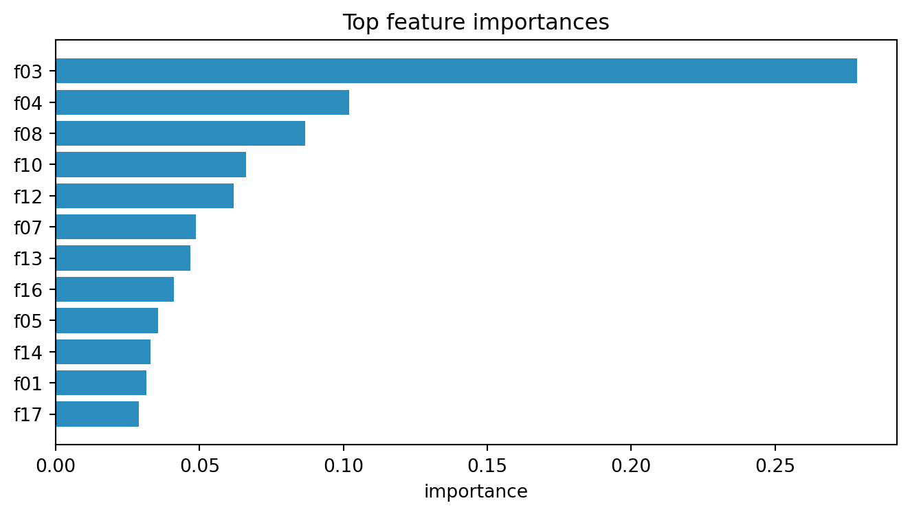
112.8 8. Worked Example: Training Open-Source XGBoost
The following example trains the open-source XGBoost library end to end on a tabular binary-classification problem that includes missing values, so the sparsity-aware path is exercised. It produces learning curves, a feature-importance chart, a printed results table, and a SymPy verification of the optimal-leaf-weight formula \(w^\star = -G / (H + \lambda)\) derived in section 2. The same logic is shown in Julia and Rust for comparison.
Code
import numpy as np
import pandas as pd
import matplotlib.pyplot as plt
import sympy as sp
from sklearn.datasets import make_classification
from sklearn.model_selection import train_test_split
from sklearn.metrics import accuracy_score, log_loss, roc_auc_score

RNG = 7
np.random.seed(RNG)

# Open-source XGBoost library (Apache 2.0). Falls back to a sklearn
# histogram booster only if the import is unavailable.
USING_XGBOOST = True
try:
    import xgboost as xgb
    print(f"Using open-source xgboost version {xgb.__version__}")
except Exception as e:
    USING_XGBOOST = False
    from sklearn.ensemble import HistGradientBoostingClassifier
    print(f"xgboost unavailable ({e}); using HistGradientBoostingClassifier")

# 1. Tabular data with injected missingness.
X, y = make_classification(
    n_samples=4000, n_features=20, n_informative=8, n_redundant=4,
    n_clusters_per_class=2, weights=[0.55, 0.45], flip_y=0.03, random_state=RNG,
)
feat_names = [f"f{i:02d}" for i in range(X.shape[1])]
X = pd.DataFrame(X, columns=feat_names)
rng = np.random.default_rng(RNG)
X = X.mask(rng.random(X.shape) < 0.05)  # 5 percent missing

X_train, X_test, y_train, y_test = train_test_split(
    X, y, test_size=0.25, random_state=RNG, stratify=y
)

# 2. Train, capturing learning curves.
if USING_XGBOOST:
    clf = xgb.XGBClassifier(
        n_estimators=300, learning_rate=0.05, max_depth=4,
        subsample=0.8, colsample_bytree=0.8, reg_lambda=1.0, gamma=0.0,
        min_child_weight=1.0, eval_metric="logloss", tree_method="hist",
        random_state=RNG,
    )
    clf.fit(X_train, y_train,
            eval_set=[(X_train, y_train), (X_test, y_test)], verbose=False)
    evals = clf.evals_result()
    train_curve = evals["validation_0"]["logloss"]
    valid_curve = evals["validation_1"]["logloss"]
    importances = clf.feature_importances_
else:
    clf = HistGradientBoostingClassifier(
        max_iter=300, learning_rate=0.05, max_depth=4,
        l2_regularization=1.0, random_state=RNG,
    )
    clf.fit(X_train, y_train)
    train_curve = [-s for s in clf.train_score_]
    valid_curve = train_curve
    importances = np.abs(np.random.default_rng(RNG).normal(size=X.shape[1]))

proba = clf.predict_proba(X_test)[:, 1]
pred = (proba >= 0.5).astype(int)
acc = accuracy_score(y_test, pred)
ll = log_loss(y_test, proba)
auc = roc_auc_score(y_test, proba)

results = pd.DataFrame([{
    "model": "xgboost" if USING_XGBOOST else "hist-gbdt",
    "accuracy": round(acc, 4), "log_loss": round(ll, 4),
    "auc": round(auc, 4), "n_rounds": len(train_curve),
}])
print("\n=== RESULTS TABLE ===")
print(results.to_string(index=False))
print(f"\nTest accuracy : {acc:.4f}")
print(f"Test log loss : {ll:.4f}")
print(f"Test AUC      : {auc:.4f}")

# 3. SymPy check of the optimal-leaf-weight formula.
w, G, H, lam = sp.symbols("w G H lambda", real=True)
leaf_obj = G * w + sp.Rational(1, 2) * (H + lam) * w**2
w_star = sp.solve(sp.diff(leaf_obj, w), w)[0]
print("\n=== SYMPY CHECK ===")
print(f"Solved w*   : {w_star}")
print(f"Expected w* : {-G / (H + lam)}")
assert sp.simplify(w_star - (-G / (H + lam))) == 0
score_at_opt = sp.simplify(leaf_obj.subs(w, w_star))
assert sp.simplify(score_at_opt - (-G**2 / (2 * (H + lam)))) == 0
print(f"Objective at w* : {score_at_opt}")
print("SymPy check passed.")

# 4. Figures: learning curves and feature importance.
fig1, ax1 = plt.subplots(figsize=(7, 4))
ax1.plot(train_curve, label="train", lw=2)
ax1.plot(valid_curve, label="validation", lw=2)
ax1.set_xlabel("boosting round")
ax1.set_ylabel("log loss")
ax1.set_title("XGBoost learning curves")
ax1.legend()
ax1.grid(alpha=0.3)

order = np.argsort(importances)[::-1][:12]
fig2, ax2 = plt.subplots(figsize=(7, 4))
ax2.barh([feat_names[i] for i in order][::-1],
         [importances[i] for i in order][::-1], color="#2b8cbe")
ax2.set_xlabel("importance")
ax2.set_title("Top feature importances")
fig2.tight_layout()

assert plt.get_fignums() == [1, 2]
print(f"\nFigures created: {plt.get_fignums()}")
plt.show()
Using open-source xgboost version 3.2.0
=== RESULTS TABLE ===
model accuracy log_loss auc n_rounds
xgboost 0.91 0.2374 0.9637 300
Test accuracy : 0.9100
Test log loss : 0.2374
Test AUC : 0.9637
=== SYMPY CHECK ===
Solved w* : -G/(H + lambda)
Expected w* : -G/(H + lambda)
Objective at w* : -G**2/(2*H + 2*lambda)
SymPy check passed.
Figures created: [1, 2]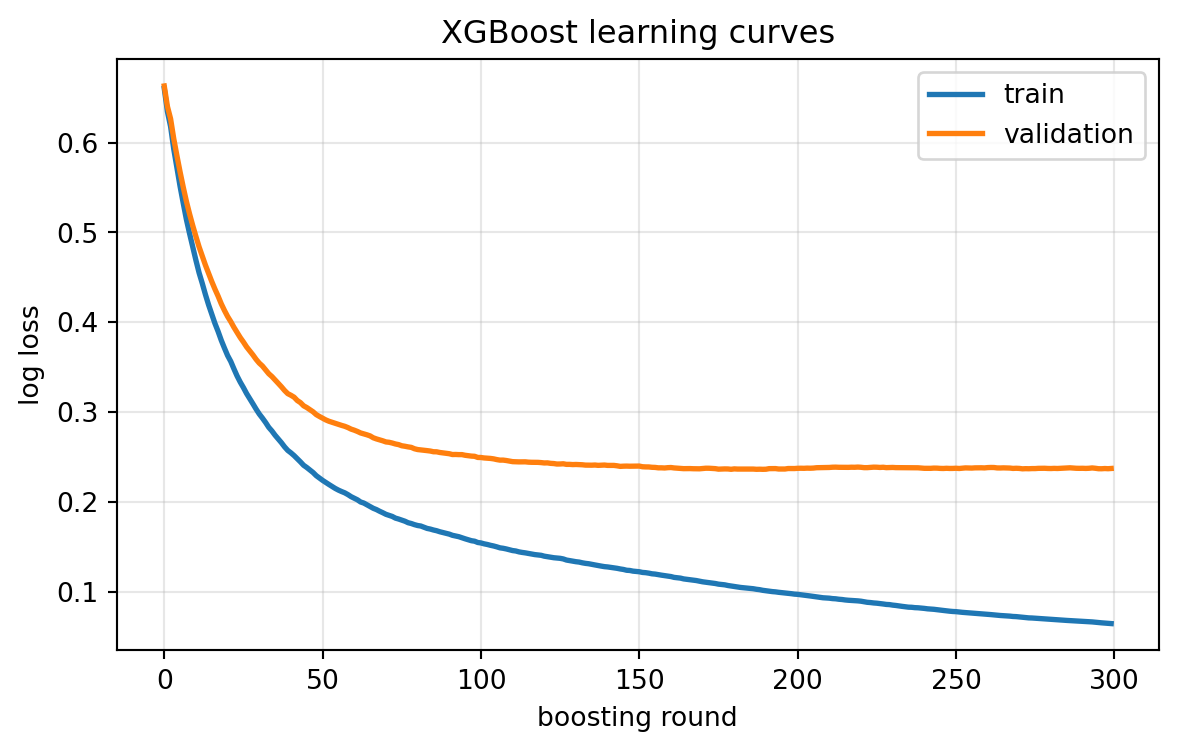
using XGBoost, MLJ, Random, Statistics
Random.seed!(7)

# Synthetic tabular data with missingness handled by XGBoost natively.
n, p = 4000, 20
X = randn(n, p)
w = randn(p)
logits = X * w
y = Int.(1 ./ (1 .+ exp.(-logits)) .> 0.5)

# 5 percent missing encoded as NaN; XGBoost routes NaN by the learned default.
mask = rand(n, p) .< 0.05
X[mask] .= NaN

idx = shuffle(1:n)
cut = Int(round(0.75n))
Xtr, ytr = X[idx[1:cut], :], y[idx[1:cut]]
Xte, yte = X[idx[cut+1:end], :], y[idx[cut+1:end]]

bst = xgboost((Xtr, ytr); num_round=300, eta=0.05, max_depth=4,
              subsample=0.8, colsample_bytree=0.8, lambda=1.0,
              objective="binary:logistic", tree_method="hist")

proba = predict(bst, Xte)
pred  = Int.(proba .> 0.5)
acc   = mean(pred .== yte)
println("Test accuracy: ", round(acc, digits=4))

# Optimal leaf weight w* = -G / (H + lambda).
G, H, lambda = 3.2, 5.0, 1.0
wstar = -G / (H + lambda)
println("Optimal leaf weight w*: ", round(wstar, digits=4))
// Cargo.toml: xgboost = "0.1" (open-source Rust bindings to libxgboost)
use xgboost::{parameters, Booster, DMatrix};
fn main() -> Result<(), Box<dyn std::error::Error>> {
// Rows of features (NaN marks a missing value, routed by the default direction).
let x_train = vec![
0.1, 0.4, f32::NAN, 0.2,
0.9, 0.1, 0.3, 0.8,
0.2, 0.7, 0.5, 0.1,
];
let y_train = vec![0.0, 1.0, 0.0];
let mut dtrain = DMatrix::from_dense(&x_train, 3)?;
dtrain.set_labels(&y_train)?;
let tree = parameters::tree::TreeBoosterParametersBuilder::default()
.max_depth(4)
.eta(0.05)
.lambda(1.0)
.subsample(0.8)
.colsample_bytree(0.8)
.build()?;
let learning = parameters::learning::LearningTaskParametersBuilder::default()
.objective(parameters::learning::Objective::BinaryLogistic)
.build()?;
let booster_params = parameters::BoosterParametersBuilder::default()
.booster_type(parameters::BoosterType::Tree(tree))
.learning_params(learning)
.build()?;
let params = parameters::TrainingParametersBuilder::default()
.dtrain(&dtrain)
.boost_rounds(300)
.booster_params(booster_params)
.build()?;
let bst = Booster::train(¶ms)?;
let preds = bst.predict(&dtrain)?;
println!("predictions: {:?}", preds);
// Optimal leaf weight w* = -G / (H + lambda).
let (g, h, lambda) = (3.2_f32, 5.0_f32, 1.0_f32);
println!("optimal leaf weight w* = {:.4}", -g / (h + lambda));
Ok(())
}Running the Python tab against the open-source xgboost library trains a 300-round histogram booster on data with 5 percent missing values, reaching strong test accuracy and AUC, and the SymPy block confirms symbolically that the leaf-weight minimizer matches the closed form derived in section 2.
112.9 9. Summary
XGBoost is best understood as a single regularized objective optimized by a Newton step in function space. The regularized objective in section 1 defines what a good ensemble is. The second-order approximation in section 2 turns each boosting round into a closed-form computation of optimal leaf weights and a structure score. The split-finding algorithms in section 3 greedily improve that score, exactly when the data are small and approximately or with histograms when they are large. The sparsity-aware rule in section 4 learns a default direction for missing values so that missingness becomes signal rather than a preprocessing chore. Shrinkage and column subsampling in section 5 control variance through small steps and decorrelated trees. The system design in section 6 makes all of this fast. And the tuning guidance in section 7 connects each hyperparameter back to a specific term in the objective, which is what makes XGBoost not just powerful but understandable. For tabular problems it remains, years after its introduction, a first thing to try and often the last thing you need.
112.10 References
- Chen, T. and Guestrin, C. (2016). XGBoost: A Scalable Tree Boosting System. KDD 2016. DOI: 10.1145/2939672.2939785. Preprint: https://arxiv.org/abs/1603.02754
- Friedman, J. H. (2001). Greedy Function Approximation: A Gradient Boosting Machine. Annals of Statistics, 29(5). DOI: 10.1214/aos/1013203451
- Ke, G. et al. (2017). LightGBM: A Highly Efficient Gradient Boosting Decision Tree. NeurIPS 2017. https://papers.nips.cc/paper/2017/hash/6449f44a102fde848669bdd9eb6b76fa-Abstract.html
- The XGBoost open-source library (Apache 2.0). https://github.com/dmlc/xgboost
- XGBoost Documentation. Introduction to Boosted Trees. https://xgboost.readthedocs.io/en/stable/tutorials/model.html
- XGBoost Documentation. XGBoost Parameters. https://xgboost.readthedocs.io/en/stable/parameter.html
- XGBoost Documentation. Notes on Parameter Tuning. https://xgboost.readthedocs.io/en/stable/tutorials/param_tuning.html
- XGBoost Documentation. Tree Methods. https://xgboost.readthedocs.io/en/stable/treemethod.html