Binary logistic regression is the workhorse of supervised classification. It models the probability that an observation belongs to one of two classes as a smooth function of a linear combination of features. Despite its simplicity, it remains a default baseline in industry and a conceptual cornerstone, because it cleanly connects linear models, probability theory, information theory, and convex optimization. This chapter develops the model from first principles, derives its training objective through maximum likelihood, shows that this objective coincides with cross entropy, and works through both gradient based and Newton (IRLS) optimization. We close with decision boundaries and the interpretation of fitted coefficients.
92.1 1. From Linear Scores to Probabilities
92.1.1 1.1 The classification setting
We observe a dataset of \(n\) labeled examples \(\{(\mathbf{x}_i, y_i)\}_{i=1}^{n}\), where \(\mathbf{x}_i \in \mathbb{R}^{d}\) is a feature vector and \(y_i \in \{0, 1\}\) is a binary label. Our goal is to learn a function that maps a feature vector to an estimate of \(P(y = 1 \mid \mathbf{x})\), the conditional probability that the positive class occurs.
A naive approach would fit ordinary linear regression directly to the labels, predicting \(\hat{y} = \mathbf{w}^{\top}\mathbf{x} + b\). This fails for two reasons. First, the linear score ranges over all of \(\mathbb{R}\), so it cannot be read as a probability bounded in \([0, 1]\). Second, the squared error loss implied by linear regression is a poor match for a Bernoulli outcome, and it heavily penalizes confident correct predictions that lie far from the boundary. We need a model that squashes a real valued score into a valid probability.
92.1.2 1.2 The sigmoid function
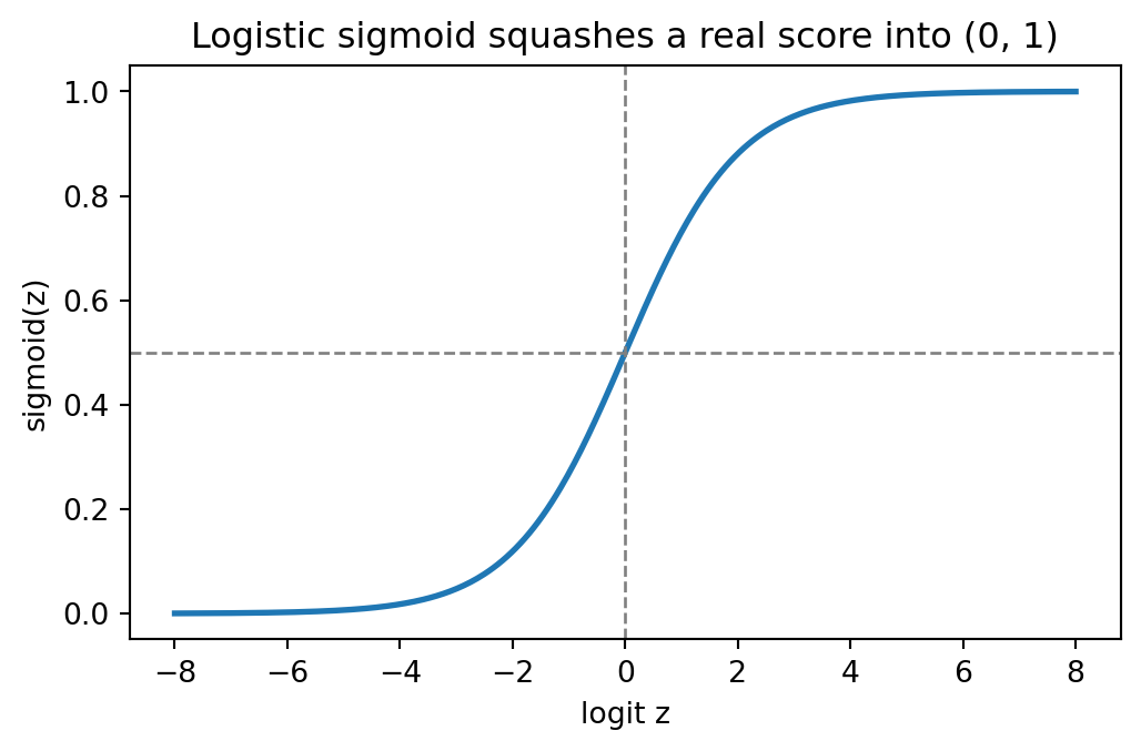
The logistic sigmoid accomplishes exactly this squashing. Define the linear score, often called the logit or activation,
\[
z = \mathbf{w}^{\top}\mathbf{x} + b,
\]
and pass it through
\[
\sigma(z) = \frac{1}{1 + e^{-z}}.
\]
The sigmoid is a monotonically increasing function from \(\mathbb{R}\) onto the open interval \((0, 1)\). It satisfies \(\sigma(0) = 1/2\), \(\sigma(z) \to 1\) as \(z \to +\infty\), and \(\sigma(z) \to 0\) as \(z \to -\infty\). Two algebraic identities are used constantly:
To lighten notation we absorb the bias into the weight vector by appending a constant feature of \(1\) to every \(\mathbf{x}\), so that \(z = \mathbf{w}^{\top}\mathbf{x}\) with the convention that \(w_0 = b\) and \(x_0 = 1\). From here on \(\mathbf{w} \in \mathbb{R}^{d+1}\).
Code
import numpy as npimport matplotlib.pyplot as pltdef sigmoid(z):# numerically stable form avoids overflow for large negative zreturn np.where(z >=0, 1/ (1+ np.exp(-z)), np.exp(z) / (1+ np.exp(z)))z = np.linspace(-8, 8, 400)fig, ax = plt.subplots(figsize=(6, 3.5))ax.plot(z, sigmoid(z), color="C0", lw=2)ax.axhline(0.5, color="gray", ls="--", lw=1)ax.axvline(0.0, color="gray", ls="--", lw=1)ax.set_xlabel("logit z")ax.set_ylabel("sigmoid(z)")ax.set_title("Logistic sigmoid squashes a real score into (0, 1)")plt.show()print("sigmoid(0) =", sigmoid(0.0))
sigmoid(0) = 0.5
92.2 2. The Log Odds Model
92.2.1 2.1 Odds and the logit link
The quantity \(p / (1 - p)\) is the odds of the positive class. A probability of \(0.8\) corresponds to odds of \(4\), meaning the event is four times as likely to occur as not. Taking the logarithm gives the log odds, also called the logit:
This is why logistic regression is a generalized linear model. The response is Bernoulli distributed, and the canonical link function connecting the mean of the response to the linear predictor is the logit. Linearity lives on the log odds scale, not on the probability scale, where the relationship is the characteristic S shaped curve.
92.2.2 2.2 Why the log odds scale is natural
Working on the log odds scale has three practical benefits. It maps the bounded interval \((0, 1)\) onto the entire real line, so the linear predictor never produces an invalid probability. It is symmetric: swapping the roles of the two classes flips the sign of the logit but leaves the structure intact. And it gives coefficients a clean multiplicative meaning in terms of odds ratios, which we develop in Section 7. The log odds representation also reveals that the decision boundary, where the two classes are equally probable, is exactly the set where \(\mathbf{w}^{\top}\mathbf{x} = 0\), a hyperplane.
92.3 3. Maximum Likelihood Estimation
92.3.1 3.1 The Bernoulli likelihood
Logistic regression estimates \(\mathbf{w}\) by maximum likelihood. Each label is modeled as a Bernoulli draw with success probability \(p_i = \sigma(\mathbf{w}^{\top}\mathbf{x}_i)\). The probability mass function for a single observation, written compactly for both outcomes, is
Products of many small probabilities underflow numerically and are awkward to differentiate, so we maximize the log likelihood instead. Because logarithm is monotonic, the maximizer is unchanged.
Maximizing \(\ell(\mathbf{w})\) is equivalent to minimizing its negative. The negative log likelihood, averaged over the dataset, is the loss we actually minimize:
92.4 4. Cross Entropy and the Connection to Information Theory
92.4.1 4.1 Cross entropy as the same objective
The loss \(J(\mathbf{w})\) is precisely the binary cross entropy between the empirical label distribution and the model. For a single example, treat the true label as a degenerate distribution placing mass \(y_i\) on class \(1\) and \(1 - y_i\) on class \(0\), and the prediction as the distribution \((p_i, 1 - p_i)\). The cross entropy between these two distributions is
which is exactly the per example term in \(J\). So maximum likelihood for the Bernoulli model and cross entropy minimization are two names for the same thing. This is no coincidence. Minimizing cross entropy is equivalent to minimizing the Kullback Leibler divergence from the model to the data generating distribution, and the maximum likelihood estimator is the one whose model distribution is closest to the empirical distribution in KL divergence.
92.4.2 4.2 Why not squared error
One might ask why we do not minimize \(\sum_i (y_i - p_i)^2\) instead. The answer is twofold. First, with \(p_i = \sigma(z_i)\), the squared error is non convex in \(\mathbf{w}\), so gradient descent can stall in poor local minima. Cross entropy composed with the sigmoid is convex, as we show next. Second, squared error produces vanishing gradients when a prediction is confidently wrong, because the sigmoid saturates and its derivative tends to zero, whereas the cross entropy gradient remains well behaved. These two properties, convexity and healthy gradients, are why cross entropy is the standard objective for classification.
92.4.3 4.3 Convexity
The objective \(J(\mathbf{w})\) is convex in \(\mathbf{w}\). Each term is a composition of the convex softplus function \(\log(1 + e^{z})\) with an affine map, since after simplification the per example loss for label \(y_i\) can be written \(\log(1 + e^{z_i}) - y_i z_i\) with \(z_i = \mathbf{w}^{\top}\mathbf{x}_i\). The Hessian, derived in Section 6, is positive semidefinite everywhere, which confirms convexity. Convexity guarantees that any local minimum is global, so first and second order methods both converge to the same optimum, assuming it exists.
92.5 5. Gradient Based Optimization
92.5.1 5.1 The gradient
To minimize \(J(\mathbf{w})\) we need its gradient. Start from a single example and use the chain rule together with the sigmoid derivative identity. With \(p_i = \sigma(z_i)\) and \(z_i = \mathbf{w}^{\top}\mathbf{x}_i\), the derivative of the loss with respect to the logit collapses to a strikingly simple form:
The intermediate \(\sigma'\) terms cancel exactly. The residual \(p_i - y_i\) is the difference between the predicted probability and the observed label. By the chain rule, \(\partial z_i / \partial \mathbf{w} = \mathbf{x}_i\), so the full gradient of the averaged loss is
where \(\mathbf{X}\) is the \(n \times (d+1)\) design matrix whose rows are the \(\mathbf{x}_i^{\top}\), and \(\mathbf{p}\), \(\mathbf{y}\) are the stacked vectors of predictions and labels. This is the same gradient form as linear regression, with the residual now defined through the sigmoid.
92.5.2 5.2 Gradient descent
Gradient descent updates the weights against the gradient with a step size, or learning rate, \(\eta > 0\):
Because \(J\) is convex with Lipschitz continuous gradient, gradient descent converges to the global minimum for a sufficiently small fixed step size. In practice the features should be standardized so that the curvature is similar in all directions, which lets a single learning rate work well. Stochastic and mini batch variants replace the full sum with an estimate from a subset of examples, trading gradient accuracy for cheaper and more frequent updates, which is essential at scale.
Code
# Two Gaussian blobs, one per class, with a bias column appended to X.rng = np.random.default_rng(0)n =200X0 = rng.normal([-1.5, -1.0], 1.0, size=(n //2, 2))X1 = rng.normal([1.5, 1.0], 1.0, size=(n //2, 2))X = np.vstack([X0, X1])y = np.concatenate([np.zeros(n //2), np.ones(n //2)])Xb = np.hstack([np.ones((len(X), 1)), X]) # column of ones is the bias featuredef train_gd(X, y, eta=0.1, steps=500): w = np.zeros(X.shape[1]) n =len(y)for _ inrange(steps): p = sigmoid(X @ w) grad = X.T @ (p - y) / n w -= eta * gradreturn ww_gd = train_gd(Xb, y)acc_gd = ((sigmoid(Xb @ w_gd) >=0.5) == y).mean()print("gradient descent weights [bias, w1, w2]:", np.round(w_gd, 3))print("training accuracy:", acc_gd)
When features are numerous or collinear, or when the classes are linearly separable, the unregularized maximum likelihood weights can grow without bound, because pushing the logits toward \(\pm\infty\) drives the loss arbitrarily low. Adding an L2 penalty \(\tfrac{\lambda}{2}\lVert \mathbf{w} \rVert^2\) to the objective keeps the weights finite, strictly convexifies the problem so the solution is unique, and corresponds to a Gaussian prior on the weights in a Bayesian reading. The penalized gradient simply adds \(\lambda \mathbf{w}\), usually excluding the bias term from the penalty.
92.6 6. Newton’s Method and Iteratively Reweighted Least Squares
92.6.1 6.1 The Hessian
Second order methods use curvature to take better steps. Differentiating the gradient again gives the Hessian. Define the diagonal weight matrix \(\mathbf{S}\) with entries \(s_{ii} = p_i(1 - p_i)\), the variance of each Bernoulli prediction. Then
Because each \(s_{ii} \ge 0\), the matrix \(\mathbf{X}^{\top}\mathbf{S}\mathbf{X}\) is positive semidefinite, which proves the convexity claimed earlier. It is positive definite, and the minimizer unique, when \(\mathbf{X}\) has full column rank and no prediction is exactly \(0\) or \(1\).
92.6.2 6.2 The Newton update
Newton’s method minimizes the local quadratic approximation of \(J\) at each step, giving the update
\[
\mathbf{w}^{(t+1)} = \mathbf{w}^{(t)} - \mathbf{H}^{-1} \nabla_{\mathbf{w}} J.
\]
Near the optimum Newton’s method converges quadratically, often reaching high accuracy in well under ten iterations, far fewer than gradient descent needs. The cost per iteration is higher because it forms and inverts the \((d+1) \times (d+1)\) Hessian, an \(O(d^3)\) operation, which makes it attractive for moderate dimensional problems and less so for very high dimensional ones.
92.6.3 6.3 IRLS as weighted least squares
The Newton update for logistic regression has an elegant interpretation as iteratively reweighted least squares. Substituting the gradient and Hessian and rearranging, each Newton step is the solution of a weighted least squares problem,
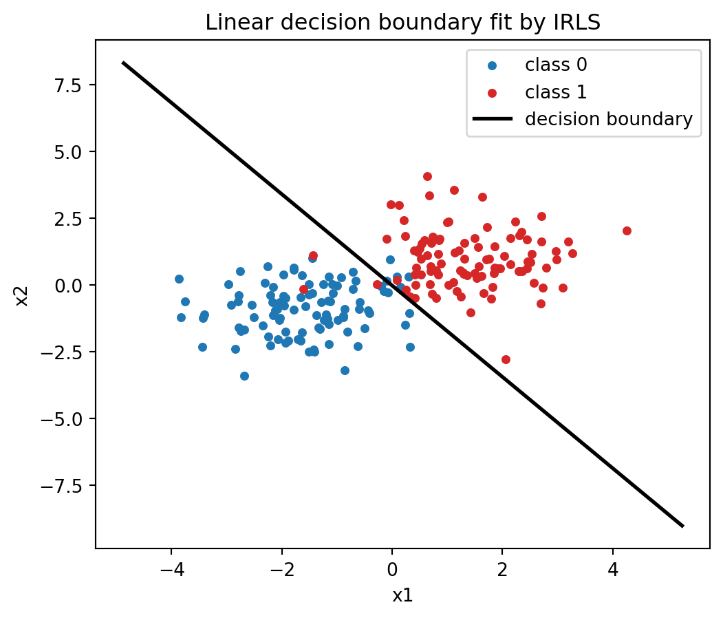
Each iteration thus fits a weighted linear regression of the working response \(\mathbf{r}\) on the features, with weights \(s_{ii} = p_i(1 - p_i)\), then recomputes the predictions and weights and repeats. Observations near the decision boundary, where \(p_i \approx 1/2\), carry the largest weight, while confident predictions near \(0\) or \(1\) contribute little, since the model has already explained them. This is the algorithm used by classical statistical software to fit generalized linear models.
Code
def train_irls(X, y, iters=10): w = np.zeros(X.shape[1])for _ inrange(iters): p = sigmoid(X @ w) s = p * (1- p)# working response and weighted normal equations z = X @ w + (y - p) / np.clip(s, 1e-8, None) H = X.T @ (s[:, None] * X) w = np.linalg.solve(H, X.T @ (s * z))return ww_irls = train_irls(Xb, y)print("IRLS weights [bias, w1, w2]:", np.round(w_irls, 3))# The decision boundary is the line w0 + w1*x1 + w2*x2 = 0.fig, ax = plt.subplots(figsize=(6, 5))ax.scatter(X[y ==0, 0], X[y ==0, 1], s=15, color="C0", label="class 0")ax.scatter(X[y ==1, 0], X[y ==1, 1], s=15, color="C3", label="class 1")xx = np.linspace(X[:, 0].min() -1, X[:, 0].max() +1, 200)yy =-(w_irls[0] + w_irls[1] * xx) / w_irls[2]ax.plot(xx, yy, "k-", lw=2, label="decision boundary")ax.set_xlabel("x1")ax.set_ylabel("x2")ax.set_title("Linear decision boundary fit by IRLS")ax.legend()plt.show()
IRLS weights [bias, w1, w2]: [0.032 2.922 1.707]
92.7 7. Decision Boundaries and Interpretation
92.7.1 7.1 The decision boundary
To turn probabilities into class predictions we apply a threshold \(\tau\), predicting class \(1\) when \(p(\mathbf{x}) \ge \tau\). The default threshold \(\tau = 1/2\) corresponds to predicting the more probable class. Since \(\sigma\) is monotone and \(\sigma(0) = 1/2\), the threshold of \(1/2\) on probability is equivalent to a threshold of \(0\) on the logit, so the decision boundary is the hyperplane
\[
\mathbf{w}^{\top}\mathbf{x} = 0.
\]
This is a linear boundary in feature space. Logistic regression is therefore a linear classifier: it can only separate classes with a flat boundary in the given features. The orientation of the boundary is set by the weight vector, which is normal to the hyperplane, and the signed distance of a point from the boundary is proportional to its logit, so points far from the boundary receive confident probabilities near \(0\) or \(1\). Nonlinear boundaries are obtained by engineering nonlinear features, such as polynomial or interaction terms, after which the model is still linear in the expanded feature space.
92.7.2 7.2 Choosing the threshold
The threshold need not be \(1/2\). When classes are imbalanced or when the costs of false positives and false negatives differ, the operating threshold should be chosen to optimize the relevant criterion, such as expected cost, the F1 score, or a target on precision or recall. Crucially, the fitted probabilities themselves do not change with the threshold; only the classification rule applied to them does. Tools such as the receiver operating characteristic curve and the precision recall curve summarize performance across all thresholds at once.
92.7.3 7.3 Interpreting coefficients
The coefficients carry a precise meaning on the odds scale. Holding all other features fixed, increasing feature \(j\) by one unit adds \(w_j\) to the log odds, which multiplies the odds by \(e^{w_j}\). The quantity \(e^{w_j}\) is the odds ratio associated with that feature. A coefficient of \(0.7\), for instance, means each unit increase in the feature multiplies the odds of the positive class by about \(e^{0.7} \approx 2.0\), doubling them. A coefficient of \(0\) means the feature leaves the odds unchanged. The sign tells the direction of the effect, and the magnitude, once features are standardized, indicates relative importance.
Two cautions apply. The effect is constant on the log odds scale but not on the probability scale, where the same coefficient produces a larger change near \(p = 1/2\) and a smaller change in the saturated tails. And these are associations within the model, not causal effects, and they depend on which other features are included, since logistic coefficients are adjusted for the other covariates in the model.
92.7.4 7.4 Calibration
A valuable property of logistic regression trained by maximum likelihood is that its predicted probabilities tend to be well calibrated: among examples assigned probability around \(0.3\), roughly \(30\) percent are truly positive. This follows from the fact that minimizing cross entropy is a proper scoring rule, rewarding honest probabilities rather than merely correct rankings. Calibration makes the outputs directly usable in downstream decision making, expected value calculations, and risk estimates, which is one reason logistic regression endures even where more flexible classifiers are available.
92.8 8. Summary
Binary logistic regression assumes the log odds of the positive class are linear in the features, which is equivalent to passing a linear score through the sigmoid to obtain a probability. The model is fit by maximum likelihood, whose negative log likelihood is exactly the binary cross entropy, a convex objective with a clean gradient equal to the feature weighted residual \(p - y\). Optimization can proceed by gradient descent, which is cheap and scalable, or by Newton’s method, which appears as iteratively reweighted least squares and converges in a handful of iterations for moderate dimensions. The resulting classifier has a linear decision boundary, coefficients interpretable as odds ratios, and probability outputs that are typically well calibrated. These properties make it the canonical baseline for binary classification and the building block from which softmax regression, generalized linear models, and the output layers of neural networks are constructed.
92.9 References
Hastie, T., Tibshirani, R., and Friedman, J. The Elements of Statistical Learning, 2nd ed. Springer, 2009. https://hastie.su.domains/ElemStatLearn/
Bishop, C. M. Pattern Recognition and Machine Learning. Springer, 2006. https://www.microsoft.com/en-us/research/publication/pattern-recognition-machine-learning/
McCullagh, P., and Nelder, J. A. Generalized Linear Models, 2nd ed. Chapman and Hall, 1989. https://doi.org/10.1201/9780203753736
Murphy, K. P. Probabilistic Machine Learning: An Introduction. MIT Press, 2022. https://probml.github.io/pml-book/book1.html
Ng, A. CS229 Lecture Notes: Supervised Learning and Logistic Regression. Stanford University. https://cs229.stanford.edu/main_notes.pdf
Boyd, S., and Vandenberghe, L. Convex Optimization. Cambridge University Press, 2004. https://web.stanford.edu/~boyd/cvxbook/
Pedregosa, F., et al. Scikit learn: Logistic Regression User Guide. https://scikit-learn.org/stable/modules/linear_model.html#logistic-regression
Source Code
# Binary Logistic RegressionBinary logistic regression is the workhorse of supervised classification. It models the probability that an observation belongs to one of two classes as a smooth function of a linear combination of features. Despite its simplicity, it remains a default baseline in industry and a conceptual cornerstone, because it cleanly connects linear models, probability theory, information theory, and convex optimization. This chapter develops the model from first principles, derives its training objective through maximum likelihood, shows that this objective coincides with cross entropy, and works through both gradient based and Newton (IRLS) optimization. We close with decision boundaries and the interpretation of fitted coefficients.## 1. From Linear Scores to Probabilities### 1.1 The classification settingWe observe a dataset of $n$ labeled examples $\{(\mathbf{x}_i, y_i)\}_{i=1}^{n}$, where $\mathbf{x}_i \in \mathbb{R}^{d}$ is a feature vector and $y_i \in \{0, 1\}$ is a binary label. Our goal is to learn a function that maps a feature vector to an estimate of $P(y = 1 \mid \mathbf{x})$, the conditional probability that the positive class occurs.A naive approach would fit ordinary linear regression directly to the labels, predicting $\hat{y} = \mathbf{w}^{\top}\mathbf{x} + b$. This fails for two reasons. First, the linear score ranges over all of $\mathbb{R}$, so it cannot be read as a probability bounded in $[0, 1]$. Second, the squared error loss implied by linear regression is a poor match for a Bernoulli outcome, and it heavily penalizes confident correct predictions that lie far from the boundary. We need a model that squashes a real valued score into a valid probability.### 1.2 The sigmoid functionThe logistic sigmoid accomplishes exactly this squashing. Define the linear score, often called the logit or activation,$$z = \mathbf{w}^{\top}\mathbf{x} + b,$$and pass it through$$\sigma(z) = \frac{1}{1 + e^{-z}}.$$The sigmoid is a monotonically increasing function from $\mathbb{R}$ onto the open interval $(0, 1)$. It satisfies $\sigma(0) = 1/2$, $\sigma(z) \to 1$ as $z \to +\infty$, and $\sigma(z) \to 0$ as $z \to -\infty$. Two algebraic identities are used constantly:$$1 - \sigma(z) = \sigma(-z), \qquad \sigma'(z) = \sigma(z)\bigl(1 - \sigma(z)\bigr).$$The derivative identity is what makes logistic regression so clean to optimize. The model probability is then$$p(\mathbf{x}) = P(y = 1 \mid \mathbf{x}) = \sigma(\mathbf{w}^{\top}\mathbf{x} + b).$$To lighten notation we absorb the bias into the weight vector by appending a constant feature of $1$ to every $\mathbf{x}$, so that $z = \mathbf{w}^{\top}\mathbf{x}$ with the convention that $w_0 = b$ and $x_0 = 1$. From here on $\mathbf{w} \in \mathbb{R}^{d+1}$.```{python}import numpy as npimport matplotlib.pyplot as pltdef sigmoid(z):# numerically stable form avoids overflow for large negative zreturn np.where(z >=0, 1/ (1+ np.exp(-z)), np.exp(z) / (1+ np.exp(z)))z = np.linspace(-8, 8, 400)fig, ax = plt.subplots(figsize=(6, 3.5))ax.plot(z, sigmoid(z), color="C0", lw=2)ax.axhline(0.5, color="gray", ls="--", lw=1)ax.axvline(0.0, color="gray", ls="--", lw=1)ax.set_xlabel("logit z")ax.set_ylabel("sigmoid(z)")ax.set_title("Logistic sigmoid squashes a real score into (0, 1)")plt.show()print("sigmoid(0) =", sigmoid(0.0))```## 2. The Log Odds Model### 2.1 Odds and the logit linkThe quantity $p / (1 - p)$ is the odds of the positive class. A probability of $0.8$ corresponds to odds of $4$, meaning the event is four times as likely to occur as not. Taking the logarithm gives the log odds, also called the logit:$$\operatorname{logit}(p) = \log \frac{p}{1 - p}.$$The logit is the inverse of the sigmoid. Substituting $p = \sigma(z)$ and using $1 - \sigma(z) = \sigma(-z)$,$$\log \frac{\sigma(z)}{1 - \sigma(z)} = \log \frac{\sigma(z)}{\sigma(-z)} = \log e^{z} = z.$$This is the defining structural assumption of logistic regression: the log odds of the positive class are a linear function of the features.$$\log \frac{P(y = 1 \mid \mathbf{x})}{P(y = 0 \mid \mathbf{x})} = \mathbf{w}^{\top}\mathbf{x}.$$This is why logistic regression is a generalized linear model. The response is Bernoulli distributed, and the canonical link function connecting the mean of the response to the linear predictor is the logit. Linearity lives on the log odds scale, not on the probability scale, where the relationship is the characteristic S shaped curve.### 2.2 Why the log odds scale is naturalWorking on the log odds scale has three practical benefits. It maps the bounded interval $(0, 1)$ onto the entire real line, so the linear predictor never produces an invalid probability. It is symmetric: swapping the roles of the two classes flips the sign of the logit but leaves the structure intact. And it gives coefficients a clean multiplicative meaning in terms of odds ratios, which we develop in Section 7. The log odds representation also reveals that the decision boundary, where the two classes are equally probable, is exactly the set where $\mathbf{w}^{\top}\mathbf{x} = 0$, a hyperplane.## 3. Maximum Likelihood Estimation### 3.1 The Bernoulli likelihoodLogistic regression estimates $\mathbf{w}$ by maximum likelihood. Each label is modeled as a Bernoulli draw with success probability $p_i = \sigma(\mathbf{w}^{\top}\mathbf{x}_i)$. The probability mass function for a single observation, written compactly for both outcomes, is$$P(y_i \mid \mathbf{x}_i; \mathbf{w}) = p_i^{\,y_i} (1 - p_i)^{1 - y_i}.$$Assuming the observations are independent given the features, the likelihood of the full dataset is the product$$L(\mathbf{w}) = \prod_{i=1}^{n} p_i^{\,y_i} (1 - p_i)^{1 - y_i}.$$### 3.2 The log likelihoodProducts of many small probabilities underflow numerically and are awkward to differentiate, so we maximize the log likelihood instead. Because logarithm is monotonic, the maximizer is unchanged.$$\ell(\mathbf{w}) = \sum_{i=1}^{n} \Bigl[ y_i \log p_i + (1 - y_i) \log (1 - p_i) \Bigr].$$Maximizing $\ell(\mathbf{w})$ is equivalent to minimizing its negative. The negative log likelihood, averaged over the dataset, is the loss we actually minimize:$$J(\mathbf{w}) = -\frac{1}{n} \sum_{i=1}^{n} \Bigl[ y_i \log p_i + (1 - y_i) \log (1 - p_i) \Bigr].$$## 4. Cross Entropy and the Connection to Information Theory### 4.1 Cross entropy as the same objectiveThe loss $J(\mathbf{w})$ is precisely the binary cross entropy between the empirical label distribution and the model. For a single example, treat the true label as a degenerate distribution placing mass $y_i$ on class $1$ and $1 - y_i$ on class $0$, and the prediction as the distribution $(p_i, 1 - p_i)$. The cross entropy between these two distributions is$$H(y_i, p_i) = -\bigl[ y_i \log p_i + (1 - y_i) \log (1 - p_i) \bigr],$$which is exactly the per example term in $J$. So maximum likelihood for the Bernoulli model and cross entropy minimization are two names for the same thing. This is no coincidence. Minimizing cross entropy is equivalent to minimizing the Kullback Leibler divergence from the model to the data generating distribution, and the maximum likelihood estimator is the one whose model distribution is closest to the empirical distribution in KL divergence.### 4.2 Why not squared errorOne might ask why we do not minimize $\sum_i (y_i - p_i)^2$ instead. The answer is twofold. First, with $p_i = \sigma(z_i)$, the squared error is non convex in $\mathbf{w}$, so gradient descent can stall in poor local minima. Cross entropy composed with the sigmoid is convex, as we show next. Second, squared error produces vanishing gradients when a prediction is confidently wrong, because the sigmoid saturates and its derivative tends to zero, whereas the cross entropy gradient remains well behaved. These two properties, convexity and healthy gradients, are why cross entropy is the standard objective for classification.### 4.3 ConvexityThe objective $J(\mathbf{w})$ is convex in $\mathbf{w}$. Each term is a composition of the convex softplus function $\log(1 + e^{z})$ with an affine map, since after simplification the per example loss for label $y_i$ can be written $\log(1 + e^{z_i}) - y_i z_i$ with $z_i = \mathbf{w}^{\top}\mathbf{x}_i$. The Hessian, derived in Section 6, is positive semidefinite everywhere, which confirms convexity. Convexity guarantees that any local minimum is global, so first and second order methods both converge to the same optimum, assuming it exists.## 5. Gradient Based Optimization### 5.1 The gradientTo minimize $J(\mathbf{w})$ we need its gradient. Start from a single example and use the chain rule together with the sigmoid derivative identity. With $p_i = \sigma(z_i)$ and $z_i = \mathbf{w}^{\top}\mathbf{x}_i$, the derivative of the loss with respect to the logit collapses to a strikingly simple form:$$\frac{\partial}{\partial z_i} \Bigl[ -y_i \log p_i - (1 - y_i)\log(1 - p_i) \Bigr] = p_i - y_i.$$The intermediate $\sigma'$ terms cancel exactly. The residual $p_i - y_i$ is the difference between the predicted probability and the observed label. By the chain rule, $\partial z_i / \partial \mathbf{w} = \mathbf{x}_i$, so the full gradient of the averaged loss is$$\nabla_{\mathbf{w}} J = \frac{1}{n} \sum_{i=1}^{n} (p_i - y_i)\,\mathbf{x}_i = \frac{1}{n} \mathbf{X}^{\top}(\mathbf{p} - \mathbf{y}),$$where $\mathbf{X}$ is the $n \times (d+1)$ design matrix whose rows are the $\mathbf{x}_i^{\top}$, and $\mathbf{p}$, $\mathbf{y}$ are the stacked vectors of predictions and labels. This is the same gradient form as linear regression, with the residual now defined through the sigmoid.### 5.2 Gradient descentGradient descent updates the weights against the gradient with a step size, or learning rate, $\eta > 0$:$$\mathbf{w}^{(t+1)} = \mathbf{w}^{(t)} - \eta \, \nabla_{\mathbf{w}} J\bigl(\mathbf{w}^{(t)}\bigr).$$Because $J$ is convex with Lipschitz continuous gradient, gradient descent converges to the global minimum for a sufficiently small fixed step size. In practice the features should be standardized so that the curvature is similar in all directions, which lets a single learning rate work well. Stochastic and mini batch variants replace the full sum with an estimate from a subset of examples, trading gradient accuracy for cheaper and more frequent updates, which is essential at scale.```{python}# Two Gaussian blobs, one per class, with a bias column appended to X.rng = np.random.default_rng(0)n =200X0 = rng.normal([-1.5, -1.0], 1.0, size=(n //2, 2))X1 = rng.normal([1.5, 1.0], 1.0, size=(n //2, 2))X = np.vstack([X0, X1])y = np.concatenate([np.zeros(n //2), np.ones(n //2)])Xb = np.hstack([np.ones((len(X), 1)), X]) # column of ones is the bias featuredef train_gd(X, y, eta=0.1, steps=500): w = np.zeros(X.shape[1]) n =len(y)for _ inrange(steps): p = sigmoid(X @ w) grad = X.T @ (p - y) / n w -= eta * gradreturn ww_gd = train_gd(Xb, y)acc_gd = ((sigmoid(Xb @ w_gd) >=0.5) == y).mean()print("gradient descent weights [bias, w1, w2]:", np.round(w_gd, 3))print("training accuracy:", acc_gd)```### 5.3 RegularizationWhen features are numerous or collinear, or when the classes are linearly separable, the unregularized maximum likelihood weights can grow without bound, because pushing the logits toward $\pm\infty$ drives the loss arbitrarily low. Adding an L2 penalty $\tfrac{\lambda}{2}\lVert \mathbf{w} \rVert^2$ to the objective keeps the weights finite, strictly convexifies the problem so the solution is unique, and corresponds to a Gaussian prior on the weights in a Bayesian reading. The penalized gradient simply adds $\lambda \mathbf{w}$, usually excluding the bias term from the penalty.## 6. Newton's Method and Iteratively Reweighted Least Squares### 6.1 The HessianSecond order methods use curvature to take better steps. Differentiating the gradient again gives the Hessian. Define the diagonal weight matrix $\mathbf{S}$ with entries $s_{ii} = p_i(1 - p_i)$, the variance of each Bernoulli prediction. Then$$\mathbf{H} = \nabla^2_{\mathbf{w}} J = \frac{1}{n} \sum_{i=1}^{n} p_i (1 - p_i)\, \mathbf{x}_i \mathbf{x}_i^{\top} = \frac{1}{n}\mathbf{X}^{\top}\mathbf{S}\,\mathbf{X}.$$Because each $s_{ii} \ge 0$, the matrix $\mathbf{X}^{\top}\mathbf{S}\mathbf{X}$ is positive semidefinite, which proves the convexity claimed earlier. It is positive definite, and the minimizer unique, when $\mathbf{X}$ has full column rank and no prediction is exactly $0$ or $1$.### 6.2 The Newton updateNewton's method minimizes the local quadratic approximation of $J$ at each step, giving the update$$\mathbf{w}^{(t+1)} = \mathbf{w}^{(t)} - \mathbf{H}^{-1} \nabla_{\mathbf{w}} J.$$Near the optimum Newton's method converges quadratically, often reaching high accuracy in well under ten iterations, far fewer than gradient descent needs. The cost per iteration is higher because it forms and inverts the $(d+1) \times (d+1)$ Hessian, an $O(d^3)$ operation, which makes it attractive for moderate dimensional problems and less so for very high dimensional ones.### 6.3 IRLS as weighted least squaresThe Newton update for logistic regression has an elegant interpretation as iteratively reweighted least squares. Substituting the gradient and Hessian and rearranging, each Newton step is the solution of a weighted least squares problem,$$\mathbf{w}^{(t+1)} = \bigl(\mathbf{X}^{\top}\mathbf{S}\mathbf{X}\bigr)^{-1}\mathbf{X}^{\top}\mathbf{S}\,\mathbf{r},$$where the working response, or adjusted dependent variable, is$$\mathbf{r} = \mathbf{X}\mathbf{w}^{(t)} + \mathbf{S}^{-1}(\mathbf{y} - \mathbf{p}).$$Each iteration thus fits a weighted linear regression of the working response $\mathbf{r}$ on the features, with weights $s_{ii} = p_i(1 - p_i)$, then recomputes the predictions and weights and repeats. Observations near the decision boundary, where $p_i \approx 1/2$, carry the largest weight, while confident predictions near $0$ or $1$ contribute little, since the model has already explained them. This is the algorithm used by classical statistical software to fit generalized linear models.```{python}def train_irls(X, y, iters=10): w = np.zeros(X.shape[1])for _ inrange(iters): p = sigmoid(X @ w) s = p * (1- p)# working response and weighted normal equations z = X @ w + (y - p) / np.clip(s, 1e-8, None) H = X.T @ (s[:, None] * X) w = np.linalg.solve(H, X.T @ (s * z))return ww_irls = train_irls(Xb, y)print("IRLS weights [bias, w1, w2]:", np.round(w_irls, 3))# The decision boundary is the line w0 + w1*x1 + w2*x2 = 0.fig, ax = plt.subplots(figsize=(6, 5))ax.scatter(X[y ==0, 0], X[y ==0, 1], s=15, color="C0", label="class 0")ax.scatter(X[y ==1, 0], X[y ==1, 1], s=15, color="C3", label="class 1")xx = np.linspace(X[:, 0].min() -1, X[:, 0].max() +1, 200)yy =-(w_irls[0] + w_irls[1] * xx) / w_irls[2]ax.plot(xx, yy, "k-", lw=2, label="decision boundary")ax.set_xlabel("x1")ax.set_ylabel("x2")ax.set_title("Linear decision boundary fit by IRLS")ax.legend()plt.show()```## 7. Decision Boundaries and Interpretation### 7.1 The decision boundaryTo turn probabilities into class predictions we apply a threshold $\tau$, predicting class $1$ when $p(\mathbf{x}) \ge \tau$. The default threshold $\tau = 1/2$ corresponds to predicting the more probable class. Since $\sigma$ is monotone and $\sigma(0) = 1/2$, the threshold of $1/2$ on probability is equivalent to a threshold of $0$ on the logit, so the decision boundary is the hyperplane$$\mathbf{w}^{\top}\mathbf{x} = 0.$$This is a linear boundary in feature space. Logistic regression is therefore a linear classifier: it can only separate classes with a flat boundary in the given features. The orientation of the boundary is set by the weight vector, which is normal to the hyperplane, and the signed distance of a point from the boundary is proportional to its logit, so points far from the boundary receive confident probabilities near $0$ or $1$. Nonlinear boundaries are obtained by engineering nonlinear features, such as polynomial or interaction terms, after which the model is still linear in the expanded feature space.### 7.2 Choosing the thresholdThe threshold need not be $1/2$. When classes are imbalanced or when the costs of false positives and false negatives differ, the operating threshold should be chosen to optimize the relevant criterion, such as expected cost, the F1 score, or a target on precision or recall. Crucially, the fitted probabilities themselves do not change with the threshold; only the classification rule applied to them does. Tools such as the receiver operating characteristic curve and the precision recall curve summarize performance across all thresholds at once.### 7.3 Interpreting coefficientsThe coefficients carry a precise meaning on the odds scale. Holding all other features fixed, increasing feature $j$ by one unit adds $w_j$ to the log odds, which multiplies the odds by $e^{w_j}$. The quantity $e^{w_j}$ is the odds ratio associated with that feature. A coefficient of $0.7$, for instance, means each unit increase in the feature multiplies the odds of the positive class by about $e^{0.7} \approx 2.0$, doubling them. A coefficient of $0$ means the feature leaves the odds unchanged. The sign tells the direction of the effect, and the magnitude, once features are standardized, indicates relative importance.Two cautions apply. The effect is constant on the log odds scale but not on the probability scale, where the same coefficient produces a larger change near $p = 1/2$ and a smaller change in the saturated tails. And these are associations within the model, not causal effects, and they depend on which other features are included, since logistic coefficients are adjusted for the other covariates in the model.### 7.4 CalibrationA valuable property of logistic regression trained by maximum likelihood is that its predicted probabilities tend to be well calibrated: among examples assigned probability around $0.3$, roughly $30$ percent are truly positive. This follows from the fact that minimizing cross entropy is a proper scoring rule, rewarding honest probabilities rather than merely correct rankings. Calibration makes the outputs directly usable in downstream decision making, expected value calculations, and risk estimates, which is one reason logistic regression endures even where more flexible classifiers are available.## 8. SummaryBinary logistic regression assumes the log odds of the positive class are linear in the features, which is equivalent to passing a linear score through the sigmoid to obtain a probability. The model is fit by maximum likelihood, whose negative log likelihood is exactly the binary cross entropy, a convex objective with a clean gradient equal to the feature weighted residual $p - y$. Optimization can proceed by gradient descent, which is cheap and scalable, or by Newton's method, which appears as iteratively reweighted least squares and converges in a handful of iterations for moderate dimensions. The resulting classifier has a linear decision boundary, coefficients interpretable as odds ratios, and probability outputs that are typically well calibrated. These properties make it the canonical baseline for binary classification and the building block from which softmax regression, generalized linear models, and the output layers of neural networks are constructed.## References1. Hastie, T., Tibshirani, R., and Friedman, J. The Elements of Statistical Learning, 2nd ed. Springer, 2009. https://hastie.su.domains/ElemStatLearn/2. Bishop, C. M. Pattern Recognition and Machine Learning. Springer, 2006. https://www.microsoft.com/en-us/research/publication/pattern-recognition-machine-learning/3. McCullagh, P., and Nelder, J. A. Generalized Linear Models, 2nd ed. Chapman and Hall, 1989. https://doi.org/10.1201/97802037537364. Murphy, K. P. Probabilistic Machine Learning: An Introduction. MIT Press, 2022. https://probml.github.io/pml-book/book1.html5. Ng, A. CS229 Lecture Notes: Supervised Learning and Logistic Regression. Stanford University. https://cs229.stanford.edu/main_notes.pdf6. Boyd, S., and Vandenberghe, L. Convex Optimization. Cambridge University Press, 2004. https://web.stanford.edu/~boyd/cvxbook/7. Pedregosa, F., et al. Scikit learn: Logistic Regression User Guide. https://scikit-learn.org/stable/modules/linear_model.html#logistic-regression