flowchart TD
A["Initialize the distribution"] --> B["Train weak learner under current distribution"]
B --> C["Compute the weighted error"]
C --> D["Compute the confidence weight"]
D --> E["Reweight the distribution"]
E --> F{"More rounds remain"}
F -->|yes| B
F -->|no| G["Output the combined classifier"]
110 AdaBoost: Reweighting, Exponential Loss, and the Mystery of Resistance to Overfitting
AdaBoost, short for Adaptive Boosting, is one of the most influential algorithms in the history of machine learning. Introduced by Freund and Schapire in 1995, it answered a theoretical question with surprising practical force: can a collection of weak learners, each only slightly better than random guessing, be combined into a strong learner with arbitrarily low error? The answer was yes, and the resulting procedure turned out to be simple, efficient, and remarkably accurate on real data. This chapter develops AdaBoost from three complementary perspectives. We start with the algorithm itself and the intuition of reweighting, then recast it as forward stagewise minimization of an exponential loss, and finally confront the puzzle that drove a decade of theoretical work: why AdaBoost so often keeps improving its test performance even after it has perfectly classified the training set.
110.1 1. The Boosting Question and the Algorithm
110.1.1 1.1 Weak learners and the strong learning goal
A weak learner is any procedure that, given a weighted training set, returns a classifier whose weighted error is bounded below \(1/2\) by some margin. Decision stumps, which are one-level decision trees that threshold a single feature, are the canonical example. Individually they are crude. The boosting question, posed by Kearns and Valiant, asks whether the weak learning condition is equivalent to strong learning, where we demand low error with high probability. Schapire first showed the equivalence constructively, and AdaBoost made the construction practical.
The setting is binary classification with labels encoded as \(y_i \in \{-1, +1\}\). We have a training set \(\{(x_i, y_i)\}_{i=1}^{n}\) and access to a base learner that produces classifiers \(h: \mathcal{X} \to \{-1, +1\}\). The goal is a final classifier of the form
\[ H(x) = \operatorname{sign}\!\left( \sum_{t=1}^{T} \alpha_t h_t(x) \right), \]
a weighted vote over \(T\) base classifiers, where each \(\alpha_t \ge 0\) is a confidence coefficient.
110.1.2 1.2 The AdaBoost procedure
AdaBoost maintains a distribution \(D_t\) over the training examples. Initially every example is equally weighted. At each round the base learner is trained to minimize weighted error under \(D_t\), the round confidence \(\alpha_t\) is computed from that error, and the distribution is updated so that misclassified examples gain weight and correctly classified examples lose weight. The next base learner is therefore forced to attend to the examples that the ensemble so far finds hard.
Initialize D_1(i) = 1/n for i = 1..n
For t = 1..T:
    Train h_t on the data weighted by D_t
    Compute weighted error:
        eps_t = sum_i D_t(i) * 1[h_t(x_i) != y_i]
    Compute confidence:
        alpha_t = 0.5 * ln((1 - eps_t) / eps_t)
    Update weights:
        D_{t+1}(i) = D_t(i) * exp(-alpha_t * y_i * h_t(x_i)) / Z_t
    where Z_t normalizes D_{t+1} to sum to 1
Output H(x) = sign( sum_t alpha_t * h_t(x) )
Two design choices deserve immediate attention. First, \(\alpha_t = \tfrac{1}{2}\ln\!\big((1-\epsilon_t)/\epsilon_t\big)\) is large when \(\epsilon_t\) is small, so accurate base learners get more say in the final vote. If \(\epsilon_t = 1/2\) then \(\alpha_t = 0\) and a coin-flip learner contributes nothing. If \(\epsilon_t > 1/2\) the coefficient goes negative, which simply means we flip the classifier. Second, the multiplicative update uses the product \(y_i h_t(x_i)\), which is \(+1\) on correct examples and \(-1\) on errors. Correct examples are multiplied by \(e^{-\alpha_t}\) and errors by \(e^{+\alpha_t}\), so the weight of hard examples grows geometrically across rounds.
110.1.3 1.3 The training error bound
The original analysis gives a clean bound. Let \(\gamma_t = \tfrac{1}{2} - \epsilon_t\) be the edge of the base learner at round \(t\). Then the training error of the final classifier satisfies
\[ \frac{1}{n}\sum_{i=1}^{n} \mathbf{1}\!\left[ H(x_i) \neq y_i \right] \;\le\; \prod_{t=1}^{T} Z_t \;=\; \prod_{t=1}^{T} 2\sqrt{\epsilon_t(1-\epsilon_t)} \;\le\; \exp\!\left( -2 \sum_{t=1}^{T} \gamma_t^2 \right). \]
The proof rests on a telescoping identity. Unrolling the multiplicative update from \(D_1(i) = 1/n\) gives a closed form for the final distribution,
\[ D_{T+1}(i) = \frac{1}{n} \frac{\exp\!\big(-y_i \sum_{t=1}^{T} \alpha_t h_t(x_i)\big)}{\prod_{t=1}^{T} Z_t} = \frac{\exp\!\big(-y_i F(x_i)\big)}{n \prod_{t=1}^{T} Z_t}, \]
where \(F(x) = \sum_t \alpha_t h_t(x)\). Because \(D_{T+1}\) is a distribution it sums to one, so \(\frac{1}{n}\sum_i \exp(-y_i F(x_i)) = \prod_t Z_t\). The zero-one loss obeys \(\mathbf{1}[H(x_i) \neq y_i] = \mathbf{1}[y_i F(x_i) \le 0] \le \exp(-y_i F(x_i))\), hence
\[ \frac{1}{n}\sum_{i=1}^{n} \mathbf{1}\!\left[ H(x_i) \neq y_i \right] \le \frac{1}{n}\sum_{i=1}^{n} \exp\!\big(-y_i F(x_i)\big) = \prod_{t=1}^{T} Z_t. \]
Each normalizer evaluates to \(Z_t = \sum_i D_t(i) e^{-\alpha_t y_i h_t(x_i)} = (1-\epsilon_t) e^{-\alpha_t} + \epsilon_t e^{\alpha_t}\). Plugging the optimal \(\alpha_t = \tfrac{1}{2}\ln((1-\epsilon_t)/\epsilon_t)\) gives \(Z_t = 2\sqrt{\epsilon_t(1-\epsilon_t)}\). Writing \(\epsilon_t = \tfrac{1}{2} - \gamma_t\) yields \(Z_t = \sqrt{1 - 4\gamma_t^2} \le \exp(-2\gamma_t^2)\) by \(1 - u \le e^{-u}\), which completes the chain
\[ \prod_{t=1}^{T} Z_t = \prod_{t=1}^{T} \sqrt{1 - 4\gamma_t^2} \le \exp\!\left( -2 \sum_{t=1}^{T} \gamma_t^2 \right). \]
The practical reading is decisive: if every base learner beats random by a fixed margin \(\gamma\), the training error decays exponentially in \(T\). Weak learning really does imply strong learning.
110.2 2. The Reweighting View
110.2.1 2.1 Why reweighting works
The reweighting mechanism is the conceptual heart of AdaBoost. Each round redistributes attention toward the examples the current ensemble handles poorly. A useful invariant makes this precise. After the round-\(t\) update, the new distribution \(D_{t+1}\) assigns exactly \(1/2\) of its total mass to examples that \(h_t\) got right and \(1/2\) to examples it got wrong. To see this, note the correctly classified mass under \(D_t\) is \(1-\epsilon_t\) and is rescaled by \(e^{-\alpha_t} = \sqrt{\epsilon_t/(1-\epsilon_t)}\), while the misclassified mass \(\epsilon_t\) is rescaled by \(e^{\alpha_t} = \sqrt{(1-\epsilon_t)/\epsilon_t}\). Both products equal \(\sqrt{\epsilon_t(1-\epsilon_t)}\), so the masses are equalized.
This invariant has a sharp consequence: under \(D_{t+1}\) the previous classifier \(h_t\) has weighted error exactly \(1/2\). It is now useless on the reweighted data, which guarantees that the next base learner, if it has any edge at all, must extract genuinely new information. The reweighting forces decorrelation between successive ensemble members.
110.2.2 2.2 Reweighting versus resampling
In practice the base learner may not accept example weights. Two adaptations exist. Boosting by reweighting passes \(D_t\) directly into a weighted loss, which is exact and preferred when the base learner supports it. Boosting by resampling draws a bootstrap sample of size \(n\) from \(D_t\) and trains on the unweighted sample. Resampling introduces Monte Carlo noise but lets AdaBoost wrap around any off-the-shelf learner. Empirically the two behave similarly, and resampling occasionally helps by injecting variance that prevents the base learner from overfitting a single weighting.
110.2.3 2.3 The base learner contract
AdaBoost is a meta-algorithm and inherits the inductive bias of its base learner. The standard choice is a shallow tree. Decision stumps yield an additive model in single features and are fast, but they cannot represent feature interactions, so the ensemble of stumps behaves like a generalized additive model. Depth-two or depth-three trees capture pairwise and triple interactions and are often the sweet spot for tabular data. The requirement is only that the learner be weak in the technical sense and that it respond to the weighting; trees satisfy both because the weighted Gini or entropy split criterion naturally tracks \(D_t\).
110.3 3. The Exponential Loss and Forward Stagewise View
110.3.1 3.1 AdaBoost as additive modeling
The 1995 derivation was driven by margins and online learning. A second derivation, due to Friedman, Hastie, and Tibshirani in their “Additive Logistic Regression” paper, reframed AdaBoost as a greedy fit of an additive model under a specific loss. This statistical view is the one most useful for engineering and extension.
Consider building an additive model
\[ F_T(x) = \sum_{t=1}^{T} \alpha_t h_t(x) \]
to minimize the empirical exponential loss
\[ L(F) = \frac{1}{n} \sum_{i=1}^{n} \exp\!\big( -y_i F(x_i) \big). \]
The quantity \(m_i = y_i F(x_i)\) is the margin of example \(i\): positive when classified correctly, with magnitude measuring confidence. The exponential loss penalizes negative margins severely and rewards large positive margins with diminishing returns. Minimizing it jointly over all coefficients and base classifiers is intractable, so we fit one term at a time and never revisit earlier terms. This is forward stagewise additive modeling.
110.3.2 3.2 Deriving the AdaBoost updates
Suppose we have \(F_{t-1}\) and seek the next term \(\alpha h\). We minimize
\[ (\alpha_t, h_t) = \arg\min_{\alpha, h} \sum_{i=1}^{n} \exp\!\big( -y_i (F_{t-1}(x_i) + \alpha h(x_i)) \big). \]
Define the unnormalized weight \(w_i = \exp(-y_i F_{t-1}(x_i))\), which depends only on the model so far. The objective factors as \(\sum_i w_i \exp(-\alpha y_i h(x_i))\). Splitting the sum into correct and incorrect examples and using \(y_i h(x_i) \in \{-1,+1\}\) gives
\[ \sum_i w_i e^{-\alpha y_i h(x_i)} = e^{-\alpha}\!\!\sum_{y_i = h(x_i)}\!\! w_i + e^{\alpha}\!\!\sum_{y_i \neq h(x_i)}\!\! w_i = (e^{\alpha} - e^{-\alpha})\!\sum_i w_i \mathbf{1}[y_i \neq h(x_i)] + e^{-\alpha}\!\sum_i w_i . \]
For any fixed \(\alpha > 0\) this is minimized over \(h\) by choosing the classifier with the smallest weighted error under the normalized weights \(w_i / \sum_j w_j\). That is exactly the AdaBoost base-learner objective. Let \(\epsilon_t = \sum_i w_i \mathbf{1}[y_i \neq h_t(x_i)] / \sum_i w_i\) be that weighted error. Dividing the objective by \(\sum_i w_i\), the per-round loss as a function of \(\alpha\) is
\[ g(\alpha) = (e^{\alpha} - e^{-\alpha})\,\epsilon_t + e^{-\alpha}. \]
Setting \(g'(\alpha) = (e^{\alpha} + e^{-\alpha})\,\epsilon_t - e^{-\alpha} = 0\) gives \(e^{2\alpha} = (1-\epsilon_t)/\epsilon_t\), so
\[ \alpha_t = \frac{1}{2} \ln \frac{1 - \epsilon_t}{\epsilon_t}, \]
which is precisely the AdaBoost confidence; the second derivative \(g''(\alpha) = (e^{\alpha} - e^{-\alpha})\epsilon_t + e^{-\alpha} > 0\) confirms a minimum. The runnable section below verifies this stationary point symbolically with SymPy. Finally, the new weights are
\[ w_i^{\text{new}} = w_i \exp(-\alpha_t y_i h_t(x_i)), \]
matching the multiplicative reweighting up to the normalization \(Z_t\). The reweighting we introduced operationally is therefore nothing but the bookkeeping of the gradient of exponential loss. AdaBoost is coordinate descent on exponential loss in the space of base classifiers.
110.3.3 3.3 The population minimizer and a probabilistic reading
What is AdaBoost estimating? Minimizing the population exponential loss \(\mathbb{E}[e^{-y F(x)}]\) pointwise over \(F(x)\) gives the minimizer
\[ F^*(x) = \frac{1}{2} \ln \frac{P(y = +1 \mid x)}{P(y = -1 \mid x)}. \]
The optimal score is half the log-odds, so \(\operatorname{sign}(F^*(x))\) is the Bayes classifier and the ensemble score can be inverted to a probability estimate via \(P(y=+1\mid x) = 1/(1 + e^{-2F(x)})\). This connects AdaBoost to logistic regression: both target the log-odds, differing only in the loss used to get there. The exponential loss is more aggressive than the logistic loss against outliers, which is why LogitBoost, a variant fitting the same additive model under the logistic loss, can be more robust on noisy data.
exponential loss:  L(m) = exp(-m)
logistic loss:     L(m) = ln(1 + exp(-2m))
both are convex upper bounds on the 0/1 loss 1[m < 0]
exponential grows faster as m -> -inf, so it punishes outliers harder
110.3.4 3.4 Practical consequences of the loss view
The stagewise view turns AdaBoost into a flexible template. Replacing the exponential loss with a differentiable loss and taking functional gradient steps gives gradient boosting, which generalizes boosting to regression, ranking, and arbitrary objectives. Adding a learning rate \(\nu < 1\) that shrinks each \(\alpha_t\) slows the descent and almost always improves generalization, at the cost of more rounds. Subsampling rows and columns per round, as in stochastic gradient boosting, further regularizes. These ideas, all visible from the loss perspective, underlie modern systems such as XGBoost and LightGBM that dominate tabular learning competitions.
110.3.5 3.5 The loop as a diagram
The control flow of one boosting round, from training under \(D_t\) to the reweighted distribution \(D_{t+1}\), is shown below.
| Step | Formula |
|---|---|
| Initialize the distribution | \(D_1(i) = 1/n\) |
| Compute the weighted error | \(\epsilon_t = \sum_i D_t(i)\, \mathbf{1}[h_t(x_i) \neq y_i]\) |
| Compute the confidence weight | \(\alpha_t = 0.5 \ln\frac{1 - \epsilon_t}{\epsilon_t}\) |
| Reweight the distribution | \(D_{t+1}(i) \propto D_t(i) \exp(-\alpha_t y_i h_t(x_i))\) |
| Output the combined classifier | \(H(x) = \operatorname{sign}\left(\sum_t \alpha_t h_t(x)\right)\) |
110.4 4. AdaBoost in Practice
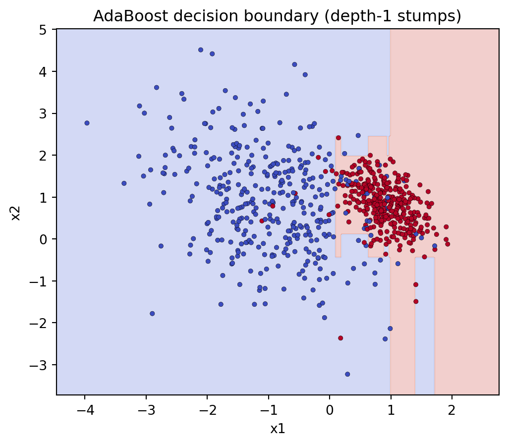
The three views above converge on one procedure. This section runs it end to end on a synthetic two-feature problem: it tracks train and test error across rounds, draws the decision boundary built from depth-one stumps, prints a results table, inspects the per-round confidence weights, and confirms the \(\alpha_t\) formula symbolically. The reference implementation is the open-source scikit-learn library.
Code
import numpy as np
import pandas as pd
import matplotlib.pyplot as plt
import sympy as sp
from sklearn.datasets import make_classification
from sklearn.ensemble import AdaBoostClassifier
from sklearn.tree import DecisionTreeClassifier
from sklearn.model_selection import train_test_split

np.random.seed(42)

X, y = make_classification(n_samples=1200, n_features=2, n_redundant=0,
                           n_informative=2, n_clusters_per_class=1,
                           class_sep=0.9, flip_y=0.05, random_state=42)
Xtr, Xte, ytr, yte = train_test_split(X, y, test_size=0.4, random_state=42)

T = 300
stump = DecisionTreeClassifier(max_depth=1, random_state=42)
clf = AdaBoostClassifier(estimator=stump, n_estimators=T,
                         learning_rate=1.0, random_state=42)
clf.fit(Xtr, ytr)

# Staged train/test error across rounds
tr_err = np.array([1 - (p == ytr).mean() for p in clf.staged_predict(Xtr)])
te_err = np.array([1 - (p == yte).mean() for p in clf.staged_predict(Xte)])
rounds = np.arange(1, len(te_err) + 1)

errs = clf.estimator_errors_      # per-round weighted error eps_t
alphas = clf.estimator_weights_   # per-round confidence alpha_t

# Printed RESULTS TABLE
idx = [1, 10, 50, 100, 200, T]
table = pd.DataFrame({
    "round": idx,
    "weighted_err": [errs[i-1] for i in idx],
    "alpha": [alphas[i-1] for i in idx],
    "train_err": [tr_err[i-1] for i in idx],
    "test_err": [te_err[i-1] for i in idx],
})
print("=== AdaBoost staged results ===")
print(table.to_string(index=False, float_format=lambda v: f"{v:.4f}"))
print(f"\nFinal train error: {tr_err[-1]:.4f}   Final test error: {te_err[-1]:.4f}")

# SymPy check: alpha = 1/2 ln((1-eps)/eps) minimizes the per-round loss
eps, a = sp.symbols('epsilon alpha', positive=True)
g = (sp.exp(a) - sp.exp(-a)) * eps + sp.exp(-a)
alpha_star = sp.simplify(sp.solve(sp.diff(g, a), a)[0])
expected = sp.Rational(1, 2) * sp.log((1 - eps) / eps)
print("\nSymPy minimizer:", alpha_star)
print("Matches 1/2 ln((1-eps)/eps):",
      sp.simplify(alpha_star - expected) == 0)

# FIGURE 1: train/test error vs rounds
fig1, ax1 = plt.subplots(figsize=(7, 4.5))
ax1.plot(rounds, tr_err, label="train error", lw=2)
ax1.plot(rounds, te_err, label="test error", lw=2)
ax1.set_xlabel("boosting rounds T")
ax1.set_ylabel("error rate")
ax1.set_title("AdaBoost: train/test error vs rounds")
ax1.legend(); ax1.grid(alpha=0.3)

# FIGURE 2: decision boundary
fig2, ax2 = plt.subplots(figsize=(6, 5))
xx, yy = np.meshgrid(
    np.linspace(X[:, 0].min() - 0.5, X[:, 0].max() + 0.5, 300),
    np.linspace(X[:, 1].min() - 0.5, X[:, 1].max() + 0.5, 300))
Z = clf.predict(np.c_[xx.ravel(), yy.ravel()]).reshape(xx.shape)
ax2.contourf(xx, yy, Z, alpha=0.25, cmap="coolwarm")
ax2.scatter(Xtr[:, 0], Xtr[:, 1], c=ytr, cmap="coolwarm",
            s=12, edgecolor="k", linewidth=0.2)
ax2.set_title("AdaBoost decision boundary (depth-1 stumps)")
ax2.set_xlabel("x1"); ax2.set_ylabel("x2")

# FIGURE 3: per-round confidence
fig3, ax3 = plt.subplots(figsize=(7, 4))
ax3.plot(rounds, alphas, color="purple", lw=1.5)
ax3.set_xlabel("round t"); ax3.set_ylabel(r"$\alpha_t$")
ax3.set_title("Per-round confidence weights")
ax3.grid(alpha=0.3)

plt.show()
=== AdaBoost staged results ===
round weighted_err alpha train_err test_err
1 0.0653 2.6616 0.0653 0.0917
10 0.4391 0.2449 0.0653 0.0917
50 0.4834 0.0665 0.0528 0.0729
100 0.4917 0.0332 0.0500 0.0708
200 0.4948 0.0206 0.0514 0.0667
300 0.4960 0.0160 0.0514 0.0667
Final train error: 0.0514 Final test error: 0.0667
SymPy minimizer: log((1 - epsilon)/epsilon)/2
Matches 1/2 ln((1-eps)/eps): True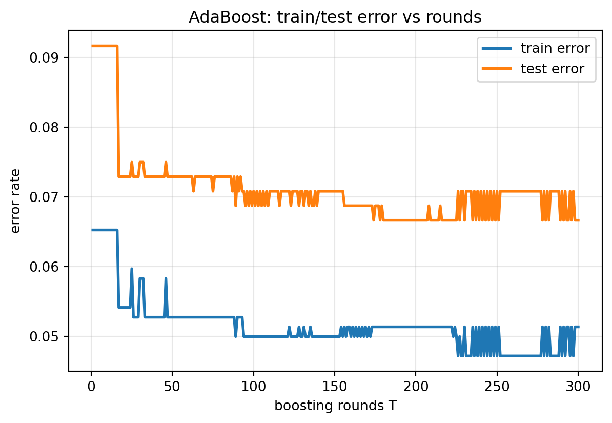

The first round earns a large \(\alpha_t\) because a single stump already separates most of the data, while later rounds drive the weighted error toward \(1/2\) and contribute small, refining \(\alpha_t\). Train error plateaus quickly, yet test error keeps drifting down as the margins widen, the signature behavior the margin theory predicts. The SymPy block confirms that the per-round loss is minimized exactly at \(\alpha_t = \tfrac{1}{2}\ln((1-\epsilon_t)/\epsilon_t)\).
using MLJ, DataFrames, Random
Random.seed!(42)

AdaBoost = @load AdaBoostStumpClassifier pkg=DecisionTree

X, y = make_blobs(1200, 2; centers=2, cluster_std=1.4, rng=42)
y = coerce(y, Multiclass)
train, test = partition(eachindex(y), 0.6; shuffle=true, rng=42)

model = AdaBoost(n_iter=300)
mach = machine(model, X, y)
fit!(mach, rows=train)

yhat = predict_mode(mach, rows=test)
test_err = mean(yhat .!= y[test])
println("Test error: ", round(test_err, digits=4))
// smartcore = "0.3"
use smartcore::ensemble::random_forest_classifier::*;
use smartcore::linalg::basic::matrix::DenseMatrix;
// smartcore has no native AdaBoost yet; the boosting loop is shown in pseudocode.
// Maintain weights D over n samples, fit a stump each round, then:
// eps = sum(D[i] for misclassified i)
// alpha = 0.5 * ((1.0 - eps) / eps).ln();
// D[i] *= (-alpha * y[i] * h[i]).exp(); // then renormalize so sum(D) == 1
// Final prediction: sign(sum_t alpha_t * h_t(x)).
fn alpha(eps: f64) -> f64 {
0.5 * ((1.0 - eps) / eps).ln()
}
fn main() {
let _x = DenseMatrix::from_2d_array(&[&[0.0_f64, 0.0]]).unwrap();
println!("alpha at eps=0.2 -> {:.4}", alpha(0.2));
}110.5 5. Why AdaBoost Resists Overfitting
110.5.1 4.1 The empirical puzzle
Classical learning theory predicts that as we add base classifiers the model complexity grows, so test error should eventually rise even as training error falls. AdaBoost repeatedly violated this expectation. In many experiments the training error reaches zero after a modest number of rounds, yet the test error keeps decreasing for hundreds or thousands of additional rounds. A model that should be overfitting instead keeps generalizing better. Explaining this became a central problem in the late 1990s.
110.5.2 4.2 The margin explanation
Schapire, Freund, Bartlett, and Lee proposed the margin theory. Define the normalized margin of example \(i\) as
\[ \operatorname{margin}(x_i, y_i) = \frac{y_i \sum_{t} \alpha_t h_t(x_i)}{\sum_{t} \alpha_t} \in [-1, 1]. \]
The sign tells us whether the example is classified correctly, and the magnitude measures the confidence of the vote. The key observation is that AdaBoost does not stop improving when the training error hits zero, because it keeps increasing the margins of examples that are already correctly classified. Pushing margins away from the decision boundary builds a buffer that generalizes.
The supporting theory bounds the generalization error in terms of the margin distribution rather than the number of rounds. With high probability,
\[ P_{\text{test}}\big( y F(x) \le 0 \big) \;\le\; P_{\text{train}}\big( \operatorname{margin}(x,y) \le \theta \big) + \tilde{O}\!\left( \sqrt{ \frac{d}{n \theta^2} } \right), \]
where \(d\) is a complexity measure of the base class and the bound holds simultaneously for all \(\theta > 0\). Critically, the right side has no explicit dependence on \(T\). If boosting keeps driving the fraction of small margins down, the bound keeps tightening even as rounds accumulate. The mechanism behind resistance to overfitting is margin maximization, not the absence of complexity.
110.5.3 4.3 The exponential loss perspective on margins
The loss view reinforces the margin story. The exponential objective \(\sum_i e^{-y_i F(x_i)}\) does not saturate once an example is correct. Even when \(y_i F(x_i) > 0\), the loss continues to decrease as the margin grows, so the optimizer has incentive to keep enlarging margins long after training error is zero. This is exactly why training error and the loss decouple: zero training error means every margin is positive, but the exponential loss can still be large if many margins are small. Continued boosting trades away that residual loss by widening the margins, which is the behavior the margin bound rewards.
110.5.4 4.4 Caveats, noise, and the limits of the story
The margin explanation is illuminating but incomplete and sometimes contested. Breiman constructed an algorithm, arc-gv, that provably maximizes the minimum margin yet generalizes worse than AdaBoost, showing that the minimum margin alone is not the whole story; the entire margin distribution matters, a point later refined by Reyzin and Schapire who noted that base classifier complexity must be controlled when comparing margins.
More importantly, AdaBoost is not immune to overfitting. Its Achilles heel is label noise. Because the exponential loss grows without bound on negative margins, a mislabeled example accrues enormous weight and the ensemble contorts itself to fit it. On noisy data AdaBoost can overfit badly, which is the practical reason to prefer robust variants such as LogitBoost, to add shrinkage, to cap the number of rounds by early stopping on a validation set, or to use soft-margin formulations that bound the influence of any single example. The honest summary is that AdaBoost resists overfitting when the base learner is weak, the data is reasonably clean, and margin maximization aligns with the true structure; it overfits when those conditions fail.
110.6 6. Putting It Together
AdaBoost rewards study because the same algorithm admits three faithful descriptions. As a reweighting scheme it is an intuitive attention mechanism that forces each new learner to confront the current ensemble’s mistakes and to decorrelate from its predecessors. As forward stagewise additive modeling it is greedy coordinate descent on the exponential loss, which exposes the confidence formula and the weight update as exact gradient bookkeeping and which links the ensemble score to the log-odds. As a margin maximizer it explains the empirical surprise that test error keeps falling past zero training error, while honestly flagging label noise as the regime where the magic breaks. For the practitioner the recipe is straightforward: use shallow trees as base learners, prefer reweighting when the learner supports it, add shrinkage and early stopping, and switch to a logistic or robust loss when the labels are dirty. For the theorist, AdaBoost remains a touchstone, the algorithm that taught the field that complexity counted in parameters can be a poor proxy for the complexity that actually governs generalization.
110.7 References
- Freund, Y. and Schapire, R. E. (1997). A Decision-Theoretic Generalization of On-Line Learning and an Application to Boosting. Journal of Computer and System Sciences. DOI: 10.1006/jcss.1997.1504
- Freund, Y. and Schapire, R. E. (1999). A Short Introduction to Boosting. Journal of Japanese Society for Artificial Intelligence. https://www.cs.princeton.edu/~schapire/papers/FreundSc99.pdf
- Friedman, J., Hastie, T., and Tibshirani, R. (2000). Additive Logistic Regression: A Statistical View of Boosting. Annals of Statistics. DOI: 10.1214/aos/1016218223
- Schapire, R. E., Freund, Y., Bartlett, P., and Lee, W. S. (1998). Boosting the Margin: A New Explanation for the Effectiveness of Voting Methods. Annals of Statistics. DOI: 10.1214/aos/1024691352
- Hastie, T., Tibshirani, R., and Friedman, J. (2009). The Elements of Statistical Learning, 2nd edition, Chapter 10. DOI: 10.1007/978-0-387-84858-7
- Schapire, R. E. and Freund, Y. (2012). Boosting: Foundations and Algorithms. MIT Press. https://mitpress.mit.edu/9780262526036/boosting/
- Reyzin, L. and Schapire, R. E. (2006). How Boosting the Margin Can Also Boost Classifier Complexity. ICML. DOI: 10.1145/1143844.1143939
- Friedman, J. (2001). Greedy Function Approximation: A Gradient Boosting Machine. Annals of Statistics. DOI: 10.1214/aos/1013203451
- Pedregosa, F. et al. (2011). Scikit-learn: Machine Learning in Python. Journal of Machine Learning Research. https://jmlr.org/papers/v12/pedregosa11a.html