Statistical estimation is the discipline of inferring properties of an unknown data generating process from a finite sample. Every machine learning model is, at its core, an estimator: it consumes data and produces a guess about some quantity, whether that quantity is a regression coefficient, a class probability, or the weights of a deep network. Understanding estimation theory therefore gives us a precise vocabulary for reasoning about what a learning algorithm is doing, how confident we should be in its output, and why some procedures generalize while others overfit. This chapter develops the classical theory of point estimation, the bias-variance decomposition, maximum likelihood, confidence intervals, and the bootstrap, and connects these ideas to the generalization behavior of modern models.
37.1 1. Point Estimators and Their Properties
37.1.1 1.1 The estimation setup
Suppose we observe data \(X_1, \dots, X_n\) drawn independently from a distribution \(P_\theta\) indexed by an unknown parameter \(\theta\). A point estimator is any function of the data, \(\hat{\theta}_n = T(X_1, \dots, X_n)\), that we use to approximate \(\theta\). Because the data are random, the estimator is itself a random variable with a distribution called the sampling distribution. The whole edifice of estimation theory amounts to characterizing this sampling distribution and choosing estimators whose distributions concentrate tightly around the truth.
A simple running example is the estimation of a population mean \(\mu = \mathbb{E}[X]\). The sample mean \(\bar{X}_n = \frac{1}{n} \sum_{i=1}^n X_i\) is the natural estimator, but it is far from the only one. We could use the median, a trimmed mean, or a shrunken version that pulls the estimate toward zero. Comparing these candidates requires criteria, and the classical criteria are bias, variance, consistency, and efficiency.
37.1.2 1.2 Bias
The bias of an estimator measures the systematic error, the gap between the average value of the estimator and the true parameter:
An estimator is unbiased when \(\mathbb{E}[\hat{\theta}_n] = \theta\) for every value of \(\theta\). The sample mean is unbiased for \(\mu\) because \(\mathbb{E}[\bar{X}_n] = \mu\) by linearity of expectation. Unbiasedness sounds desirable, and historically it was treated as a near-mandatory property, but it can be a trap. The sample variance illustrates the subtlety. The estimator
is unbiased for the population variance \(\sigma^2\), whereas the maximum likelihood version with divisor \(n\) is biased downward. The factor \(n-1\) rather than \(n\) is the famous Bessel correction, and it arises precisely because we spent one degree of freedom estimating the mean.
37.1.3 1.3 Variance and mean squared error
The variance of an estimator measures the spread of its sampling distribution:
For the sample mean of data with variance \(\sigma^2\), we have \(\text{Var}(\bar{X}_n) = \sigma^2 / n\), which shrinks as the sample grows. Bias and variance combine into a single summary of accuracy, the mean squared error:
The cross term vanishes because \(\mathbb{E}[\hat{\theta}_n - m] = 0\) by the definition of \(m\). The first surviving term is the variance and the last is the squared bias, which gives the identity. This decomposition is the cornerstone of the chapter. It says that the expected squared error of any estimator splits cleanly into a squared bias term and a variance term. Crucially, an unbiased estimator is not automatically the best estimator under MSE, because a small amount of bias can purchase a large reduction in variance. This observation, which we revisit when we discuss generalization, is what justifies regularization and shrinkage throughout machine learning.
37.1.4 1.4 Consistency
An estimator is consistent if it converges to the true parameter as the sample size grows. Formally, \(\hat{\theta}_n\) is consistent when it converges in probability:
The weak law of large numbers guarantees that the sample mean is consistent for \(\mu\) whenever the mean exists. A sufficient condition for consistency in terms of MSE is that both bias and variance vanish in the limit, since \(\text{MSE} \to 0\) implies convergence in probability by Chebyshev’s inequality. Consistency is a minimal sanity requirement. An estimator that does not improve with more data is rarely worth using, though as we will see, even inconsistent estimators are sometimes preferred when data are scarce.
37.1.5 1.5 Efficiency and the Cramer-Rao bound
Among unbiased estimators, we prefer the one with the smallest variance. The Cramer-Rao lower bound sets a floor on how small that variance can be. Define the Fisher information for a single observation as
The quantity \(s(X; \theta) = \frac{\partial}{\partial \theta} \log p(X; \theta)\) is the score. Under the standard regularity conditions that permit interchanging differentiation and integration, the score has mean zero, so the Fisher information is exactly its variance. Differentiating the identity \(\mathbb{E}[s] = 0\) once more yields the equivalent and often more convenient curvature form
which says that information is the expected sharpness of the negative log likelihood. For any unbiased estimator based on \(n\) independent observations,
The bound follows from the Cauchy-Schwarz inequality applied to the estimator and the total score \(\sum_i s(X_i; \theta)\), whose variance is \(n I(\theta)\). An unbiased estimator that attains this bound is called efficient. As a concrete instance, for the normal model with known variance \(\sigma^2\) the per-observation score is \(s = (X - \mu)/\sigma^2\), so \(I(\mu) = 1/\sigma^2\) and the bound is \(\sigma^2/n\), which the sample mean attains exactly. The sample mean is thus not merely unbiased but fully efficient for the Gaussian mean. The Fisher information quantifies how sharply the likelihood responds to changes in the parameter, so a high-information experiment permits low-variance estimation. Efficiency gives us a principled notion of optimality and motivates maximum likelihood, which achieves the bound asymptotically.
37.2 2. Maximum Likelihood Estimation
37.2.1 2.1 The likelihood principle
Maximum likelihood estimation is the most widely used general purpose estimation method, and it underlies the training of most probabilistic and neural models. Given observed data and a parametric family \(p(x; \theta)\), the likelihood function treats the data as fixed and the parameter as the variable:
\[L(\theta) = \prod_{i=1}^n p(X_i; \theta).\]
The maximum likelihood estimator is the parameter value that makes the observed data most probable:
We almost always work with the log likelihood because it turns products into sums, which is numerically stable and analytically convenient. The function \(\ell(\theta) = \sum_i \log p(X_i; \theta)\) is the objective that gradient based optimizers ascend.
37.2.2 2.2 A worked example
Consider \(n\) observations from a normal distribution with unknown mean \(\mu\) and known variance \(\sigma^2\). The log likelihood is
Differentiating with respect to \(\mu\) and setting the derivative to zero gives \(\sum_i (X_i - \mu) = 0\), so \(\hat{\mu}_{\text{MLE}} = \bar{X}_n\). The maximum likelihood estimate of the mean is just the sample average. This is reassuring, and it generalizes: minimizing squared error under a Gaussian noise assumption is equivalent to maximizing likelihood, which is why least squares regression and Gaussian maximum likelihood coincide. Likewise, the cross entropy loss minimized when training a classifier is the negative log likelihood of a categorical model, so neural network training is maximum likelihood in disguise.
37.2.3 2.3 Asymptotic properties
The deep appeal of maximum likelihood lies in its large sample behavior. Under regularity conditions, the maximum likelihood estimator is consistent, asymptotically unbiased, and asymptotically normal:
This single result says a great deal. The estimator converges to the truth, its sampling distribution becomes Gaussian, and its asymptotic variance equals the inverse Fisher information, which is exactly the Cramer-Rao bound. Maximum likelihood is therefore asymptotically efficient: no consistent estimator can do better in the limit. The result also delivers a practical recipe for uncertainty, because the inverse Fisher information, estimated from the curvature of the log likelihood at its peak, gives standard errors for the parameters. The observed information matrix, the negative Hessian of the log likelihood, is the workhorse for these calculations.
37.2.4 2.4 Caveats
Asymptotic optimality is a statement about the limit, and finite samples can behave differently. Maximum likelihood can overfit when the model is flexible relative to the data, which is the same overfitting that plagues deep networks trained to minimize negative log likelihood without regularization. The estimator can also be biased in finite samples, as the variance example showed. Finally, the regularity conditions can fail, for instance when the parameter lies on the boundary of its space or when the number of parameters grows with \(n\). These failure modes motivate penalized likelihood and Bayesian alternatives, which trade a little bias for a large gain in stability.
37.3 3. The Bias-Variance Decomposition and Generalization
37.3.1 3.1 From parameters to predictions
The bias-variance decomposition for a scalar parameter extends naturally to prediction, and this extension is where estimation theory meets machine learning directly. Suppose the true relationship is \(y = f(x) + \varepsilon\) with noise of variance \(\sigma^2\), and we fit a model \(\hat{f}\) on a random training set. For a fixed test point \(x_0\), the expected squared prediction error decomposes into three pieces:
The expectation is taken over the randomness in the training set. The first term is squared bias, the systematic error of the model class. The second is variance, the sensitivity of the fitted function to the particular training sample. The third is irreducible noise that no model can remove. This identity is the theoretical heart of generalization.
37.3.2 3.2 The tradeoff
Model complexity governs the balance between the first two terms. A simple model, such as a linear fit to curved data, has high bias because it cannot represent the truth, but low variance because it barely moves when the training data change. A highly flexible model, such as a deep tree or an overparameterized network, can fit almost any training set, driving bias toward zero, but its predictions swing wildly from one sample to the next, inflating variance. The classical picture is a U-shaped test error curve: error falls as complexity rises and bias drops, reaches a minimum, then climbs again as variance dominates. The goal of model selection is to find the complexity that minimizes the sum.
Regularization is the practical lever. Ridge regression, weight decay, dropout, and early stopping all introduce bias on purpose in order to cut variance. The MSE decomposition from Section 1 explains why this can help: if the variance reduction exceeds the squared bias introduced, total error falls. The James-Stein estimator is the classical proof of concept, demonstrating that a biased shrinkage estimator can dominate the unbiased sample mean in three or more dimensions, beating it in MSE for every value of the parameter.
37.3.3 3.3 Modern wrinkles
The clean U-shaped story has been complicated by deep learning. Very large models, trained well past the point of interpolating their training data, often continue to improve on held out data rather than degrading as the classical curve predicts. This double descent phenomenon shows test error first rising, then falling again as model size pushes beyond the interpolation threshold. The bias-variance decomposition still holds as an identity, but variance can behave non-monotonically in the overparameterized regime, partly because implicit regularization from the optimizer biases solutions toward smooth, low norm functions. The decomposition remains the right conceptual frame even as the empirical curves grow richer, and reconciling it with the observed behavior of large models is an active research area.
37.4 4. Confidence Intervals
37.4.1 4.1 Definition and interpretation
A point estimate alone is incomplete because it conveys no sense of its own uncertainty. A confidence interval is a data dependent range that contains the true parameter with a specified frequency under repeated sampling. Formally, a \(1 - \alpha\) confidence interval is a pair of statistics \((L, U)\) such that
\[P\big(L \leq \theta \leq U\big) = 1 - \alpha.\]
The interpretation requires care. The probability statement is about the random interval, not about \(\theta\), which is fixed. A 95 percent confidence interval means that if we repeated the entire experiment many times, about 95 percent of the resulting intervals would cover the true value. It does not mean that there is a 95 percent probability that this particular interval contains \(\theta\); that Bayesian style claim belongs to credible intervals, which require a prior. Conflating the two is one of the most common errors in applied statistics.
37.4.2 4.2 Constructing intervals
The standard construction for a mean uses the asymptotic normality that the central limit theorem provides. If \(\bar{X}_n\) has standard error \(\hat{\text{se}} = S / \sqrt{n}\), then an approximate \(1 - \alpha\) interval is
where \(z_{1-\alpha/2}\) is the appropriate normal quantile, equal to about \(1.96\) for 95 percent coverage. When the variance is estimated and the sample is small, the normal quantile is replaced by a Student t quantile with \(n - 1\) degrees of freedom, which widens the interval to account for the extra uncertainty in estimating \(\sigma\). The same template extends to maximum likelihood estimates through the asymptotic result of Section 2: the standard error comes from the inverse observed information, and the interval is the estimate plus or minus a normal quantile times that standard error. This is exactly how software reports confidence intervals for regression coefficients.
37.4.3 4.3 Coverage and its failures
The validity of a confidence interval rests on the accuracy of the sampling distribution used to build it. When that distribution is misspecified, coverage suffers: a nominal 95 percent interval might cover the truth only 80 percent of the time. Small samples, heavy tailed data, skewed estimators, and parameters near a boundary all degrade the normal approximation. These failures motivate methods that estimate the sampling distribution directly from the data rather than assuming a parametric form. The bootstrap is the most important such method.
37.5 5. The Bootstrap
37.5.1 5.1 The core idea
The bootstrap, introduced by Bradley Efron in 1979, is a computational method for estimating the sampling distribution of almost any statistic without analytical derivation. Its insight is that the empirical distribution of the observed sample is the best available proxy for the unknown population distribution. We cannot draw fresh samples from the population, but we can draw fresh samples from our data, treating the sample as if it were the population.
Concretely, given data \(X_1, \dots, X_n\) and a statistic \(\hat{\theta} = T(X_1, \dots, X_n)\), the nonparametric bootstrap proceeds as follows. We draw a resample of size \(n\) by sampling with replacement from the original data, producing \(X_1^*, \dots, X_n^*\). We compute the statistic on the resample to obtain \(\hat{\theta}^*\). Repeating this \(B\) times yields a collection \(\hat{\theta}^{*1}, \dots, \hat{\theta}^{*B}\) whose spread approximates the sampling distribution of \(\hat{\theta}\).
37.5.2 5.2 Standard errors and intervals
The bootstrap distribution serves two purposes. First, its standard deviation estimates the standard error of \(\hat{\theta}\):
Second, the quantiles of the bootstrap distribution yield confidence intervals. The simplest percentile interval takes the \(\alpha/2\) and \(1 - \alpha/2\) quantiles of the resampled statistics as the interval endpoints. More refined versions, such as the bias corrected and accelerated interval, adjust for skewness and bias in the bootstrap distribution and generally achieve coverage closer to nominal. The power of the approach is its generality: the same recipe handles the median, a correlation coefficient, the ratio of two parameters, or a complicated machine learning performance metric, none of which have tidy analytical standard errors.
37.5.3 5.3 When the bootstrap works and when it fails
The bootstrap is consistent under broad conditions, but it is not magic. It assumes the sample is representative, so it inherits any selection bias in the data and cannot correct for it. It can fail for statistics that depend on extreme order statistics, such as the sample maximum, because resampling never produces values beyond the observed range. It also struggles with strongly dependent data, where the independence assumed by simple resampling is violated; specialized variants such as the block bootstrap address time series and other dependent structures. Despite these caveats, the bootstrap has become indispensable, precisely because it replaces fragile analytical assumptions with computation. In machine learning it appears directly in bagging, where bootstrap resamples train an ensemble whose averaging reduces variance, a clean application of the bias-variance lessons of this chapter.
37.5.4 5.4 Bringing the threads together
The arc of this chapter runs from a single number to a full distribution. We began with point estimators and the criteria, bias, variance, consistency, and efficiency, that distinguish good ones from bad. The mean squared error decomposition revealed that bias and variance trade against each other, a tension that recurs as the central explanation for generalization in machine learning. Maximum likelihood gave a universal estimation engine with strong asymptotic guarantees, and it turned out to be the same objective minimized when training regression models and neural classifiers. Confidence intervals and the bootstrap then equipped us to quantify uncertainty, the former through parametric theory and the latter through resampling. Together these tools let a practitioner not only produce an estimate but also state honestly how much to trust it, which is the difference between a number and an inference.
37.6 6. Estimation in Code
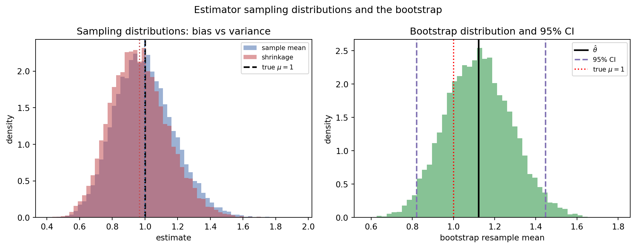
The theory becomes concrete when we simulate it. The following example draws many samples from an exponential population whose true mean is \(1\), then studies two estimators of that mean: the ordinary sample mean and a shrinkage estimator \(\hat{\mu} \cdot n / (n + k)\) that pulls the estimate gently toward zero. The simulation measures the empirical bias, variance, and mean squared error of each, confirms the decomposition numerically, and then constructs a bootstrap confidence interval from a single sample. The shrinkage estimator is deliberately biased, yet for a small penalty \(k\) its variance reduction more than pays for the bias, so its mean squared error comes in below that of the unbiased sample mean. This is the bias-variance tradeoff in miniature.
37.6.1 Python executable
Code
import numpy as npimport scipy.stats as stimport matplotlib.pyplot as pltimport sympy as sprng = np.random.default_rng(42)# True population: exponential with mean mu = 1 (so variance is also 1)true_mu =1.0n =30# sample sizereps =20000# number of simulated samplesk =1.0# shrinkage penaltymeans = np.empty(reps)shrunk = np.empty(reps)for i inrange(reps): x = rng.exponential(scale=true_mu, size=n) m = x.mean() means[i] = m shrunk[i] = m * n / (n + k) # biased, lower variancedef report(name, est, target): bias = est.mean() - target var = est.var() mse = ((est - target) **2).mean()print(f"{name:13s} bias={bias:+.4f} var={var:.4f} "f"mse={mse:.4f} (bias^2+var={bias**2+ var:.4f})")print(f"Sampling distribution over {reps} samples of size {n}")report("sample mean", means, true_mu)report("shrinkage", shrunk, true_mu)# Bootstrap confidence interval for the mean from ONE fresh samplesample = rng.exponential(scale=true_mu, size=n)theta_hat = sample.mean()B =10000boot = np.empty(B)for b inrange(B): boot[b] = rng.choice(sample, size=n, replace=True).mean()se_boot = boot.std(ddof=1)lo, hi = np.percentile(boot, [2.5, 97.5])print(f"\nOne sample: theta_hat={theta_hat:.4f}")print(f"Bootstrap SE={se_boot:.4f}")print(f"95% percentile bootstrap CI=[{lo:.4f}, {hi:.4f}] (true mu={true_mu})")# Normal-theory t-interval for comparisonse_t = sample.std(ddof=1) / np.sqrt(n)t = st.t.ppf(0.975, df=n -1)print(f"95% t-interval=[{theta_hat - t*se_t:.4f}, {theta_hat + t*se_t:.4f}]")# Symbolic check: the MSE decomposition MSE = bias^2 + var is an identity.# Verify it for the shrinkage estimator c*Xbar of an exponential(mean=mu).# E[Xbar]=mu, Var(Xbar)=mu^2/n, so for est = c*Xbar:# bias = c*mu - mu, var = c^2 * mu^2/n, mse = bias^2 + var.c, mu_s, n_s = sp.symbols("c mu n", positive=True)bias_sym = c * mu_s - mu_svar_sym = c**2* mu_s**2/ n_smse_sym = sp.expand(bias_sym**2+ var_sym)# E[(c*Xbar - mu)^2] computed directly from E[Xbar^2]=Var+mean^2:exbar2 = mu_s**2/ n_s + mu_s**2mse_direct = sp.expand(c**2* exbar2 -2* c * mu_s * mu_s + mu_s**2)assert sp.simplify(mse_sym - mse_direct) ==0print(f"\nSymPy check: MSE == bias^2 + var identity holds -> {mse_sym}")# FIGURE: sampling distributions of the two estimators (bias and variance)# plus the bootstrap distribution with its 95% percentile interval.fig, (ax1, ax2) = plt.subplots(1, 2, figsize=(11, 4.3))bins = np.linspace(min(means.min(), shrunk.min()),max(means.max(), shrunk.max()), 60)ax1.hist(means, bins=bins, density=True, alpha=0.55, color="#4C72B0", label="sample mean")ax1.hist(shrunk, bins=bins, density=True, alpha=0.55, color="#C44E52", label="shrinkage")ax1.axvline(true_mu, color="black", lw=2, ls="--", label=r"true $\mu=1$")ax1.axvline(means.mean(), color="#4C72B0", lw=1.5, ls=":")ax1.axvline(shrunk.mean(), color="#C44E52", lw=1.5, ls=":")ax1.set_xlabel("estimate")ax1.set_ylabel("density")ax1.set_title("Sampling distributions: bias vs variance")ax1.legend(fontsize=8)ax2.hist(boot, bins=50, density=True, alpha=0.7, color="#55A868")ax2.axvline(theta_hat, color="black", lw=2, label=r"$\hat{\theta}$")ax2.axvline(lo, color="#8172B3", lw=1.8, ls="--", label="95% CI")ax2.axvline(hi, color="#8172B3", lw=1.8, ls="--")ax2.axvline(true_mu, color="red", lw=1.5, ls=":", label=r"true $\mu=1$")ax2.set_xlabel("bootstrap resample mean")ax2.set_ylabel("density")ax2.set_title("Bootstrap distribution and 95% CI")ax2.legend(fontsize=8)fig.suptitle("Estimator sampling distributions and the bootstrap", fontsize=12)fig.tight_layout()plt.show()
Sampling distribution over 20000 samples of size 30
sample mean   bias=-0.0012  var=0.0333  mse=0.0333  (bias^2+var=0.0333)
shrinkage     bias=-0.0334  var=0.0312  mse=0.0323  (bias^2+var=0.0323)

One sample: theta_hat=1.1218
Bootstrap SE=0.1614
95% percentile bootstrap CI=[0.8204, 1.4464] (true mu=1.0)
95% t-interval=[0.7843, 1.4594]

SymPy check: MSE == bias^2 + var identity holds  -> c**2*mu**2 + c**2*mu**2/n - 2*c*mu**2 + mu**2
Running this prints the empirical bias, variance, and mean squared error for both estimators, showing that the sample mean is essentially unbiased while the shrinkage estimator carries a small negative bias but a lower variance, and that the sum of squared bias and variance reproduces the mean squared error to within Monte Carlo noise. The bootstrap interval, built purely by resampling with no distributional assumption, lands close to the normal theory interval and brackets the true mean of \(1\).
37.6.2 Julia
The same logic transcribes directly to Julia, whose vectorized array operations and built-in statistics make the simulation compact. This snippet is illustrative and is not executed when the book is built.
usingRandom, Statistics, Distributionsrng =MersenneTwister(42)true_mu =1.0n =30reps =20_000k =1.0means =zeros(reps)shrunk =zeros(reps)for i in1:reps x =rand(rng, Exponential(true_mu), n) m =mean(x) means[i] = m shrunk[i] = m * n / (n + k)endmse(est, target) =mean((est .- target).^2)println("sample mean bias=", mean(means) - true_mu, " mse=", mse(means, true_mu))println("shrinkage bias=", mean(shrunk) - true_mu, " mse=", mse(shrunk, true_mu))# Bootstrap confidence interval from one samplesample =rand(rng, Exponential(true_mu), n)B =10_000boot = [mean(rand(rng, sample, n)) for _ in1:B]lo, hi =quantile(boot, [0.025, 0.975])println("95% bootstrap CI = [", lo, ", ", hi, "]")
37.6.3 Rust
In Rust the same procedure is more explicit about types and random number generation, which is the price and the payoff of a systems language. This snippet is illustrative.
userand::rngs::StdRng;userand::{Rng, SeedableRng};userand_distr::{Distribution, Exp};fn mean(v:&[f64]) ->f64{ v.iter().sum::<f64>() / v.len() asf64}fn main() {letmut rng =StdRng::seed_from_u64(42);let exp =Exp::new(1.0).unwrap();// rate 1 means mean 1let (n, reps, k) = (30usize,20_000usize,1.0f64);letmut bias_mean =0.0;letmut bias_shrunk =0.0;for _ in0..reps {let x:Vec<f64>= (0..n).map(|_| exp.sample(&mut rng)).collect();let m = mean(&x); bias_mean += m; bias_shrunk += m * n asf64/ (n asf64+ k);}println!("sample mean avg = {:.4}", bias_mean / reps asf64);println!("shrinkage avg = {:.4}", bias_shrunk / reps asf64);// Bootstrap confidence interval from one samplelet sample:Vec<f64>= (0..n).map(|_| exp.sample(&mut rng)).collect();let b =10_000;letmut boot:Vec<f64>= (0..b).map(|_|{let rs:Vec<f64>= (0..n).map(|_| sample[rng.gen_range(0..n)]).collect(); mean(&rs)}).collect(); boot.sort_by(|a, c| a.partial_cmp(c).unwrap());let lo = boot[(0.025* b asf64) asusize];let hi = boot[(0.975* b asf64) asusize];println!("95% bootstrap CI = [{:.4}, {:.4}]", lo, hi);}
37.7 References
Casella, G. and Berger, R. L. (2002). Statistical Inference, 2nd edition. Duxbury Press. ISBN 978-0534243128.
Wasserman, L. (2004). All of Statistics: A Concise Course in Statistical Inference. Springer. https://doi.org/10.1007/978-0-387-21736-9
Efron, B. (1979). Bootstrap Methods: Another Look at the Jackknife. Annals of Statistics, 7(1), 1 to 26. https://doi.org/10.1214/aos/1176344552
Efron, B. and Tibshirani, R. J. (1994). An Introduction to the Bootstrap. Chapman and Hall/CRC. https://doi.org/10.1201/9780429246593
Hastie, T., Tibshirani, R., and Friedman, J. (2009). The Elements of Statistical Learning: Data Mining, Inference, and Prediction, 2nd edition. Springer. https://doi.org/10.1007/978-0-387-84858-7
James, W. and Stein, C. (1961). Estimation with Quadratic Loss. Proceedings of the Fourth Berkeley Symposium on Mathematical Statistics and Probability, 1, 361 to 379. https://projecteuclid.org/euclid.bsmsp/1200512173
Belkin, M., Hsu, D., Ma, S., and Mandal, S. (2019). Reconciling Modern Machine Learning Practice and the Classical Bias-Variance Trade-off. Proceedings of the National Academy of Sciences, 116(32), 15849 to 15854. https://doi.org/10.1073/pnas.1903070116
Lehmann, E. L. and Casella, G. (1998). Theory of Point Estimation, 2nd edition. Springer. https://doi.org/10.1007/b98854
Cramer, H. (1946). Mathematical Methods of Statistics. Princeton University Press. https://doi.org/10.1515/9781400883868
Rao, C. R. (1945). Information and the Accuracy Attainable in the Estimation of Statistical Parameters. Bulletin of the Calcutta Mathematical Society, 37, 81 to 91. Reprinted in Breakthroughs in Statistics (1992), Springer. https://doi.org/10.1007/978-1-4612-0919-5_16
Source Code
# Estimation and ConfidenceStatistical estimation is the discipline of inferring properties of an unknown data generating process from a finite sample. Every machine learning model is, at its core, an estimator: it consumes data and produces a guess about some quantity, whether that quantity is a regression coefficient, a class probability, or the weights of a deep network. Understanding estimation theory therefore gives us a precise vocabulary for reasoning about what a learning algorithm is doing, how confident we should be in its output, and why some procedures generalize while others overfit. This chapter develops the classical theory of point estimation, the bias-variance decomposition, maximum likelihood, confidence intervals, and the bootstrap, and connects these ideas to the generalization behavior of modern models.## 1. Point Estimators and Their Properties### 1.1 The estimation setupSuppose we observe data $X_1, \dots, X_n$ drawn independently from a distribution $P_\theta$ indexed by an unknown parameter $\theta$. A point estimator is any function of the data, $\hat{\theta}_n = T(X_1, \dots, X_n)$, that we use to approximate $\theta$. Because the data are random, the estimator is itself a random variable with a distribution called the sampling distribution. The whole edifice of estimation theory amounts to characterizing this sampling distribution and choosing estimators whose distributions concentrate tightly around the truth.A simple running example is the estimation of a population mean $\mu = \mathbb{E}[X]$. The sample mean $\bar{X}_n = \frac{1}{n} \sum_{i=1}^n X_i$ is the natural estimator, but it is far from the only one. We could use the median, a trimmed mean, or a shrunken version that pulls the estimate toward zero. Comparing these candidates requires criteria, and the classical criteria are bias, variance, consistency, and efficiency.### 1.2 BiasThe bias of an estimator measures the systematic error, the gap between the average value of the estimator and the true parameter:$$\text{Bias}(\hat{\theta}_n) = \mathbb{E}[\hat{\theta}_n] - \theta.$$An estimator is unbiased when $\mathbb{E}[\hat{\theta}_n] = \theta$ for every value of $\theta$. The sample mean is unbiased for $\mu$ because $\mathbb{E}[\bar{X}_n] = \mu$ by linearity of expectation. Unbiasedness sounds desirable, and historically it was treated as a near-mandatory property, but it can be a trap. The sample variance illustrates the subtlety. The estimator$$S^2 = \frac{1}{n-1} \sum_{i=1}^n (X_i - \bar{X}_n)^2$$is unbiased for the population variance $\sigma^2$, whereas the maximum likelihood version with divisor $n$ is biased downward. The factor $n-1$ rather than $n$ is the famous Bessel correction, and it arises precisely because we spent one degree of freedom estimating the mean.### 1.3 Variance and mean squared errorThe variance of an estimator measures the spread of its sampling distribution:$$\text{Var}(\hat{\theta}_n) = \mathbb{E}\big[(\hat{\theta}_n - \mathbb{E}[\hat{\theta}_n])^2\big].$$For the sample mean of data with variance $\sigma^2$, we have $\text{Var}(\bar{X}_n) = \sigma^2 / n$, which shrinks as the sample grows. Bias and variance combine into a single summary of accuracy, the mean squared error:$$\text{MSE}(\hat{\theta}_n) = \mathbb{E}\big[(\hat{\theta}_n - \theta)^2\big] = \text{Bias}(\hat{\theta}_n)^2 + \text{Var}(\hat{\theta}_n).$$The decomposition follows from adding and subtracting the mean of the estimator. Write $m = \mathbb{E}[\hat{\theta}_n]$ and expand:$$\mathbb{E}\big[(\hat{\theta}_n - \theta)^2\big] = \mathbb{E}\big[(\hat{\theta}_n - m + m - \theta)^2\big] = \mathbb{E}\big[(\hat{\theta}_n - m)^2\big] + 2(m - \theta)\,\mathbb{E}[\hat{\theta}_n - m] + (m - \theta)^2.$$The cross term vanishes because $\mathbb{E}[\hat{\theta}_n - m] = 0$ by the definition of $m$. The first surviving term is the variance and the last is the squared bias, which gives the identity. This decomposition is the cornerstone of the chapter. It says that the expected squared error of any estimator splits cleanly into a squared bias term and a variance term. Crucially, an unbiased estimator is not automatically the best estimator under MSE, because a small amount of bias can purchase a large reduction in variance. This observation, which we revisit when we discuss generalization, is what justifies regularization and shrinkage throughout machine learning.### 1.4 ConsistencyAn estimator is consistent if it converges to the true parameter as the sample size grows. Formally, $\hat{\theta}_n$ is consistent when it converges in probability:$$\hat{\theta}_n \xrightarrow{p} \theta, \quad \text{meaning} \quad \lim_{n \to \infty} P\big(|\hat{\theta}_n - \theta| > \epsilon\big) = 0 \quad \text{for every } \epsilon > 0.$$The weak law of large numbers guarantees that the sample mean is consistent for $\mu$ whenever the mean exists. A sufficient condition for consistency in terms of MSE is that both bias and variance vanish in the limit, since $\text{MSE} \to 0$ implies convergence in probability by Chebyshev's inequality. Consistency is a minimal sanity requirement. An estimator that does not improve with more data is rarely worth using, though as we will see, even inconsistent estimators are sometimes preferred when data are scarce.### 1.5 Efficiency and the Cramer-Rao boundAmong unbiased estimators, we prefer the one with the smallest variance. The Cramer-Rao lower bound sets a floor on how small that variance can be. Define the Fisher information for a single observation as$$I(\theta) = \mathbb{E}\left[\left(\frac{\partial}{\partial \theta} \log p(X; \theta)\right)^2\right].$$The quantity $s(X; \theta) = \frac{\partial}{\partial \theta} \log p(X; \theta)$ is the score. Under the standard regularity conditions that permit interchanging differentiation and integration, the score has mean zero, so the Fisher information is exactly its variance. Differentiating the identity $\mathbb{E}[s] = 0$ once more yields the equivalent and often more convenient curvature form$$I(\theta) = -\,\mathbb{E}\left[\frac{\partial^2}{\partial \theta^2} \log p(X; \theta)\right],$$which says that information is the expected sharpness of the negative log likelihood. For any unbiased estimator based on $n$ independent observations,$$\text{Var}(\hat{\theta}_n) \geq \frac{1}{n \, I(\theta)}.$$The bound follows from the Cauchy-Schwarz inequality applied to the estimator and the total score $\sum_i s(X_i; \theta)$, whose variance is $n I(\theta)$. An unbiased estimator that attains this bound is called efficient. As a concrete instance, for the normal model with known variance $\sigma^2$ the per-observation score is $s = (X - \mu)/\sigma^2$, so $I(\mu) = 1/\sigma^2$ and the bound is $\sigma^2/n$, which the sample mean attains exactly. The sample mean is thus not merely unbiased but fully efficient for the Gaussian mean. The Fisher information quantifies how sharply the likelihood responds to changes in the parameter, so a high-information experiment permits low-variance estimation. Efficiency gives us a principled notion of optimality and motivates maximum likelihood, which achieves the bound asymptotically.## 2. Maximum Likelihood Estimation### 2.1 The likelihood principleMaximum likelihood estimation is the most widely used general purpose estimation method, and it underlies the training of most probabilistic and neural models. Given observed data and a parametric family $p(x; \theta)$, the likelihood function treats the data as fixed and the parameter as the variable:$$L(\theta) = \prod_{i=1}^n p(X_i; \theta).$$The maximum likelihood estimator is the parameter value that makes the observed data most probable:$$\hat{\theta}_{\text{MLE}} = \arg\max_\theta L(\theta) = \arg\max_\theta \sum_{i=1}^n \log p(X_i; \theta).$$We almost always work with the log likelihood because it turns products into sums, which is numerically stable and analytically convenient. The function $\ell(\theta) = \sum_i \log p(X_i; \theta)$ is the objective that gradient based optimizers ascend.### 2.2 A worked exampleConsider $n$ observations from a normal distribution with unknown mean $\mu$ and known variance $\sigma^2$. The log likelihood is$$\ell(\mu) = -\frac{n}{2} \log(2 \pi \sigma^2) - \frac{1}{2 \sigma^2} \sum_{i=1}^n (X_i - \mu)^2.$$Differentiating with respect to $\mu$ and setting the derivative to zero gives $\sum_i (X_i - \mu) = 0$, so $\hat{\mu}_{\text{MLE}} = \bar{X}_n$. The maximum likelihood estimate of the mean is just the sample average. This is reassuring, and it generalizes: minimizing squared error under a Gaussian noise assumption is equivalent to maximizing likelihood, which is why least squares regression and Gaussian maximum likelihood coincide. Likewise, the cross entropy loss minimized when training a classifier is the negative log likelihood of a categorical model, so neural network training is maximum likelihood in disguise.### 2.3 Asymptotic propertiesThe deep appeal of maximum likelihood lies in its large sample behavior. Under regularity conditions, the maximum likelihood estimator is consistent, asymptotically unbiased, and asymptotically normal:$$\sqrt{n}\,(\hat{\theta}_{\text{MLE}} - \theta) \xrightarrow{d} \mathcal{N}\big(0, \, I(\theta)^{-1}\big).$$This single result says a great deal. The estimator converges to the truth, its sampling distribution becomes Gaussian, and its asymptotic variance equals the inverse Fisher information, which is exactly the Cramer-Rao bound. Maximum likelihood is therefore asymptotically efficient: no consistent estimator can do better in the limit. The result also delivers a practical recipe for uncertainty, because the inverse Fisher information, estimated from the curvature of the log likelihood at its peak, gives standard errors for the parameters. The observed information matrix, the negative Hessian of the log likelihood, is the workhorse for these calculations.### 2.4 CaveatsAsymptotic optimality is a statement about the limit, and finite samples can behave differently. Maximum likelihood can overfit when the model is flexible relative to the data, which is the same overfitting that plagues deep networks trained to minimize negative log likelihood without regularization. The estimator can also be biased in finite samples, as the variance example showed. Finally, the regularity conditions can fail, for instance when the parameter lies on the boundary of its space or when the number of parameters grows with $n$. These failure modes motivate penalized likelihood and Bayesian alternatives, which trade a little bias for a large gain in stability.## 3. The Bias-Variance Decomposition and Generalization### 3.1 From parameters to predictionsThe bias-variance decomposition for a scalar parameter extends naturally to prediction, and this extension is where estimation theory meets machine learning directly. Suppose the true relationship is $y = f(x) + \varepsilon$ with noise of variance $\sigma^2$, and we fit a model $\hat{f}$ on a random training set. For a fixed test point $x_0$, the expected squared prediction error decomposes into three pieces:$$\mathbb{E}\big[(y_0 - \hat{f}(x_0))^2\big] = \underbrace{\big(f(x_0) - \mathbb{E}[\hat{f}(x_0)]\big)^2}_{\text{bias}^2} + \underbrace{\text{Var}\big(\hat{f}(x_0)\big)}_{\text{variance}} + \underbrace{\sigma^2}_{\text{irreducible}}.$$The expectation is taken over the randomness in the training set. The first term is squared bias, the systematic error of the model class. The second is variance, the sensitivity of the fitted function to the particular training sample. The third is irreducible noise that no model can remove. This identity is the theoretical heart of generalization.### 3.2 The tradeoffModel complexity governs the balance between the first two terms. A simple model, such as a linear fit to curved data, has high bias because it cannot represent the truth, but low variance because it barely moves when the training data change. A highly flexible model, such as a deep tree or an overparameterized network, can fit almost any training set, driving bias toward zero, but its predictions swing wildly from one sample to the next, inflating variance. The classical picture is a U-shaped test error curve: error falls as complexity rises and bias drops, reaches a minimum, then climbs again as variance dominates. The goal of model selection is to find the complexity that minimizes the sum.Regularization is the practical lever. Ridge regression, weight decay, dropout, and early stopping all introduce bias on purpose in order to cut variance. The MSE decomposition from Section 1 explains why this can help: if the variance reduction exceeds the squared bias introduced, total error falls. The James-Stein estimator is the classical proof of concept, demonstrating that a biased shrinkage estimator can dominate the unbiased sample mean in three or more dimensions, beating it in MSE for every value of the parameter.### 3.3 Modern wrinklesThe clean U-shaped story has been complicated by deep learning. Very large models, trained well past the point of interpolating their training data, often continue to improve on held out data rather than degrading as the classical curve predicts. This double descent phenomenon shows test error first rising, then falling again as model size pushes beyond the interpolation threshold. The bias-variance decomposition still holds as an identity, but variance can behave non-monotonically in the overparameterized regime, partly because implicit regularization from the optimizer biases solutions toward smooth, low norm functions. The decomposition remains the right conceptual frame even as the empirical curves grow richer, and reconciling it with the observed behavior of large models is an active research area.## 4. Confidence Intervals### 4.1 Definition and interpretationA point estimate alone is incomplete because it conveys no sense of its own uncertainty. A confidence interval is a data dependent range that contains the true parameter with a specified frequency under repeated sampling. Formally, a $1 - \alpha$ confidence interval is a pair of statistics $(L, U)$ such that$$P\big(L \leq \theta \leq U\big) = 1 - \alpha.$$The interpretation requires care. The probability statement is about the random interval, not about $\theta$, which is fixed. A 95 percent confidence interval means that if we repeated the entire experiment many times, about 95 percent of the resulting intervals would cover the true value. It does not mean that there is a 95 percent probability that this particular interval contains $\theta$; that Bayesian style claim belongs to credible intervals, which require a prior. Conflating the two is one of the most common errors in applied statistics.### 4.2 Constructing intervalsThe standard construction for a mean uses the asymptotic normality that the central limit theorem provides. If $\bar{X}_n$ has standard error $\hat{\text{se}} = S / \sqrt{n}$, then an approximate $1 - \alpha$ interval is$$\bar{X}_n \pm z_{1 - \alpha/2} \, \hat{\text{se}},$$where $z_{1-\alpha/2}$ is the appropriate normal quantile, equal to about $1.96$ for 95 percent coverage. When the variance is estimated and the sample is small, the normal quantile is replaced by a Student t quantile with $n - 1$ degrees of freedom, which widens the interval to account for the extra uncertainty in estimating $\sigma$. The same template extends to maximum likelihood estimates through the asymptotic result of Section 2: the standard error comes from the inverse observed information, and the interval is the estimate plus or minus a normal quantile times that standard error. This is exactly how software reports confidence intervals for regression coefficients.### 4.3 Coverage and its failuresThe validity of a confidence interval rests on the accuracy of the sampling distribution used to build it. When that distribution is misspecified, coverage suffers: a nominal 95 percent interval might cover the truth only 80 percent of the time. Small samples, heavy tailed data, skewed estimators, and parameters near a boundary all degrade the normal approximation. These failures motivate methods that estimate the sampling distribution directly from the data rather than assuming a parametric form. The bootstrap is the most important such method.## 5. The Bootstrap### 5.1 The core ideaThe bootstrap, introduced by Bradley Efron in 1979, is a computational method for estimating the sampling distribution of almost any statistic without analytical derivation. Its insight is that the empirical distribution of the observed sample is the best available proxy for the unknown population distribution. We cannot draw fresh samples from the population, but we can draw fresh samples from our data, treating the sample as if it were the population.Concretely, given data $X_1, \dots, X_n$ and a statistic $\hat{\theta} = T(X_1, \dots, X_n)$, the nonparametric bootstrap proceeds as follows. We draw a resample of size $n$ by sampling with replacement from the original data, producing $X_1^*, \dots, X_n^*$. We compute the statistic on the resample to obtain $\hat{\theta}^*$. Repeating this $B$ times yields a collection $\hat{\theta}^{*1}, \dots, \hat{\theta}^{*B}$ whose spread approximates the sampling distribution of $\hat{\theta}$.### 5.2 Standard errors and intervalsThe bootstrap distribution serves two purposes. First, its standard deviation estimates the standard error of $\hat{\theta}$:$$\hat{\text{se}}_{\text{boot}} = \sqrt{\frac{1}{B - 1} \sum_{b=1}^B \big(\hat{\theta}^{*b} - \bar{\theta}^*\big)^2}, \quad \bar{\theta}^* = \frac{1}{B} \sum_{b=1}^B \hat{\theta}^{*b}.$$Second, the quantiles of the bootstrap distribution yield confidence intervals. The simplest percentile interval takes the $\alpha/2$ and $1 - \alpha/2$ quantiles of the resampled statistics as the interval endpoints. More refined versions, such as the bias corrected and accelerated interval, adjust for skewness and bias in the bootstrap distribution and generally achieve coverage closer to nominal. The power of the approach is its generality: the same recipe handles the median, a correlation coefficient, the ratio of two parameters, or a complicated machine learning performance metric, none of which have tidy analytical standard errors.### 5.3 When the bootstrap works and when it failsThe bootstrap is consistent under broad conditions, but it is not magic. It assumes the sample is representative, so it inherits any selection bias in the data and cannot correct for it. It can fail for statistics that depend on extreme order statistics, such as the sample maximum, because resampling never produces values beyond the observed range. It also struggles with strongly dependent data, where the independence assumed by simple resampling is violated; specialized variants such as the block bootstrap address time series and other dependent structures. Despite these caveats, the bootstrap has become indispensable, precisely because it replaces fragile analytical assumptions with computation. In machine learning it appears directly in bagging, where bootstrap resamples train an ensemble whose averaging reduces variance, a clean application of the bias-variance lessons of this chapter.### 5.4 Bringing the threads togetherThe arc of this chapter runs from a single number to a full distribution. We began with point estimators and the criteria, bias, variance, consistency, and efficiency, that distinguish good ones from bad. The mean squared error decomposition revealed that bias and variance trade against each other, a tension that recurs as the central explanation for generalization in machine learning. Maximum likelihood gave a universal estimation engine with strong asymptotic guarantees, and it turned out to be the same objective minimized when training regression models and neural classifiers. Confidence intervals and the bootstrap then equipped us to quantify uncertainty, the former through parametric theory and the latter through resampling. Together these tools let a practitioner not only produce an estimate but also state honestly how much to trust it, which is the difference between a number and an inference.## 6. Estimation in CodeThe theory becomes concrete when we simulate it. The following example draws many samples from an exponential population whose true mean is $1$, then studies two estimators of that mean: the ordinary sample mean and a shrinkage estimator $\hat{\mu} \cdot n / (n + k)$ that pulls the estimate gently toward zero. The simulation measures the empirical bias, variance, and mean squared error of each, confirms the decomposition numerically, and then constructs a bootstrap confidence interval from a single sample. The shrinkage estimator is deliberately biased, yet for a small penalty $k$ its variance reduction more than pays for the bias, so its mean squared error comes in below that of the unbiased sample mean. This is the bias-variance tradeoff in miniature.### Python executable```{python}import numpy as npimport scipy.stats as stimport matplotlib.pyplot as pltimport sympy as sprng = np.random.default_rng(42)# True population: exponential with mean mu = 1 (so variance is also 1)true_mu =1.0n =30# sample sizereps =20000# number of simulated samplesk =1.0# shrinkage penaltymeans = np.empty(reps)shrunk = np.empty(reps)for i inrange(reps): x = rng.exponential(scale=true_mu, size=n) m = x.mean() means[i] = m shrunk[i] = m * n / (n + k) # biased, lower variancedef report(name, est, target): bias = est.mean() - target var = est.var() mse = ((est - target) **2).mean()print(f"{name:13s} bias={bias:+.4f} var={var:.4f} "f"mse={mse:.4f} (bias^2+var={bias**2+ var:.4f})")print(f"Sampling distribution over {reps} samples of size {n}")report("sample mean", means, true_mu)report("shrinkage", shrunk, true_mu)# Bootstrap confidence interval for the mean from ONE fresh samplesample = rng.exponential(scale=true_mu, size=n)theta_hat = sample.mean()B =10000boot = np.empty(B)for b inrange(B): boot[b] = rng.choice(sample, size=n, replace=True).mean()se_boot = boot.std(ddof=1)lo, hi = np.percentile(boot, [2.5, 97.5])print(f"\nOne sample: theta_hat={theta_hat:.4f}")print(f"Bootstrap SE={se_boot:.4f}")print(f"95% percentile bootstrap CI=[{lo:.4f}, {hi:.4f}] (true mu={true_mu})")# Normal-theory t-interval for comparisonse_t = sample.std(ddof=1) / np.sqrt(n)t = st.t.ppf(0.975, df=n -1)print(f"95% t-interval=[{theta_hat - t*se_t:.4f}, {theta_hat + t*se_t:.4f}]")# Symbolic check: the MSE decomposition MSE = bias^2 + var is an identity.# Verify it for the shrinkage estimator c*Xbar of an exponential(mean=mu).# E[Xbar]=mu, Var(Xbar)=mu^2/n, so for est = c*Xbar:# bias = c*mu - mu, var = c^2 * mu^2/n, mse = bias^2 + var.c, mu_s, n_s = sp.symbols("c mu n", positive=True)bias_sym = c * mu_s - mu_svar_sym = c**2* mu_s**2/ n_smse_sym = sp.expand(bias_sym**2+ var_sym)# E[(c*Xbar - mu)^2] computed directly from E[Xbar^2]=Var+mean^2:exbar2 = mu_s**2/ n_s + mu_s**2mse_direct = sp.expand(c**2* exbar2 -2* c * mu_s * mu_s + mu_s**2)assert sp.simplify(mse_sym - mse_direct) ==0print(f"\nSymPy check: MSE == bias^2 + var identity holds -> {mse_sym}")# FIGURE: sampling distributions of the two estimators (bias and variance)# plus the bootstrap distribution with its 95% percentile interval.fig, (ax1, ax2) = plt.subplots(1, 2, figsize=(11, 4.3))bins = np.linspace(min(means.min(), shrunk.min()),max(means.max(), shrunk.max()), 60)ax1.hist(means, bins=bins, density=True, alpha=0.55, color="#4C72B0", label="sample mean")ax1.hist(shrunk, bins=bins, density=True, alpha=0.55, color="#C44E52", label="shrinkage")ax1.axvline(true_mu, color="black", lw=2, ls="--", label=r"true $\mu=1$")ax1.axvline(means.mean(), color="#4C72B0", lw=1.5, ls=":")ax1.axvline(shrunk.mean(), color="#C44E52", lw=1.5, ls=":")ax1.set_xlabel("estimate")ax1.set_ylabel("density")ax1.set_title("Sampling distributions: bias vs variance")ax1.legend(fontsize=8)ax2.hist(boot, bins=50, density=True, alpha=0.7, color="#55A868")ax2.axvline(theta_hat, color="black", lw=2, label=r"$\hat{\theta}$")ax2.axvline(lo, color="#8172B3", lw=1.8, ls="--", label="95% CI")ax2.axvline(hi, color="#8172B3", lw=1.8, ls="--")ax2.axvline(true_mu, color="red", lw=1.5, ls=":", label=r"true $\mu=1$")ax2.set_xlabel("bootstrap resample mean")ax2.set_ylabel("density")ax2.set_title("Bootstrap distribution and 95% CI")ax2.legend(fontsize=8)fig.suptitle("Estimator sampling distributions and the bootstrap", fontsize=12)fig.tight_layout()plt.show()```Running this prints the empirical bias, variance, and mean squared error for both estimators, showing that the sample mean is essentially unbiased while the shrinkage estimator carries a small negative bias but a lower variance, and that the sum of squared bias and variance reproduces the mean squared error to within Monte Carlo noise. The bootstrap interval, built purely by resampling with no distributional assumption, lands close to the normal theory interval and brackets the true mean of $1$.### JuliaThe same logic transcribes directly to Julia, whose vectorized array operations and built-in statistics make the simulation compact. This snippet is illustrative and is not executed when the book is built.```juliausingRandom, Statistics, Distributionsrng =MersenneTwister(42)true_mu =1.0n =30reps =20_000k =1.0means =zeros(reps)shrunk =zeros(reps)for i in1:reps x =rand(rng, Exponential(true_mu), n) m =mean(x) means[i] = m shrunk[i] = m * n / (n + k)endmse(est, target) =mean((est .- target).^2)println("sample mean bias=", mean(means) - true_mu, " mse=", mse(means, true_mu))println("shrinkage bias=", mean(shrunk) - true_mu, " mse=", mse(shrunk, true_mu))# Bootstrap confidence interval from one samplesample =rand(rng, Exponential(true_mu), n)B =10_000boot = [mean(rand(rng, sample, n)) for _ in1:B]lo, hi =quantile(boot, [0.025, 0.975])println("95% bootstrap CI = [", lo, ", ", hi, "]")```### RustIn Rust the same procedure is more explicit about types and random number generation, which is the price and the payoff of a systems language. This snippet is illustrative.```rustuse rand::rngs::StdRng;use rand::{Rng, SeedableRng};use rand_distr::{Distribution, Exp};fn mean(v:&[f64]) -> f64 {v.iter().sum::<f64>() /v.len() as f64}fn main() { let mut rng = StdRng::seed_from_u64(42); let exp = Exp::new(1.0).unwrap(); // rate 1 means mean 1let (n, reps, k) = (30usize, 20_000usize, 1.0f64); let mut bias_mean =0.0; let mut bias_shrunk =0.0;for _ in0..reps { let x: Vec<f64>= (0..n).map(|_|exp.sample(&mut rng)).collect(); let m =mean(&x); bias_mean += m; bias_shrunk += m * n as f64 / (n as f64 + k); } println!("sample mean avg = {:.4}", bias_mean / reps as f64); println!("shrinkage avg = {:.4}", bias_shrunk / reps as f64);// Bootstrap confidence interval from one sample let sample: Vec<f64>= (0..n).map(|_|exp.sample(&mut rng)).collect(); let b =10_000; let mut boot: Vec<f64>= (0..b).map(|_| { let rs: Vec<f64>= (0..n).map(|_| sample[rng.gen_range(0..n)]).collect();mean(&rs) }).collect();boot.sort_by(|a, c|a.partial_cmp(c).unwrap()); let lo = boot[(0.025* b as f64) as usize]; let hi = boot[(0.975* b as f64) as usize]; println!("95% bootstrap CI = [{:.4}, {:.4}]", lo, hi);}```## References1. Casella, G. and Berger, R. L. (2002). *Statistical Inference*, 2nd edition. Duxbury Press. ISBN 978-0534243128.2. Wasserman, L. (2004). *All of Statistics: A Concise Course in Statistical Inference*. Springer. https://doi.org/10.1007/978-0-387-21736-93. Efron, B. (1979). Bootstrap Methods: Another Look at the Jackknife. *Annals of Statistics*, 7(1), 1 to 26. https://doi.org/10.1214/aos/11763445524. Efron, B. and Tibshirani, R. J. (1994). *An Introduction to the Bootstrap*. Chapman and Hall/CRC. https://doi.org/10.1201/97804292465935. Hastie, T., Tibshirani, R., and Friedman, J. (2009). *The Elements of Statistical Learning: Data Mining, Inference, and Prediction*, 2nd edition. Springer. https://doi.org/10.1007/978-0-387-84858-76. James, W. and Stein, C. (1961). Estimation with Quadratic Loss. *Proceedings of the Fourth Berkeley Symposium on Mathematical Statistics and Probability*, 1, 361 to 379. https://projecteuclid.org/euclid.bsmsp/12005121737. Belkin, M., Hsu, D., Ma, S., and Mandal, S. (2019). Reconciling Modern Machine Learning Practice and the Classical Bias-Variance Trade-off. *Proceedings of the National Academy of Sciences*, 116(32), 15849 to 15854. https://doi.org/10.1073/pnas.19030701168. Lehmann, E. L. and Casella, G. (1998). *Theory of Point Estimation*, 2nd edition. Springer. https://doi.org/10.1007/b988549. Cramer, H. (1946). *Mathematical Methods of Statistics*. Princeton University Press. https://doi.org/10.1515/978140088386810. Rao, C. R. (1945). Information and the Accuracy Attainable in the Estimation of Statistical Parameters. *Bulletin of the Calcutta Mathematical Society*, 37, 81 to 91. Reprinted in *Breakthroughs in Statistics* (1992), Springer. https://doi.org/10.1007/978-1-4612-0919-5_16