A pre-trained language model is a good next-token predictor and a poor assistant. It will happily continue a prompt with something fluent, plausible, and useless, because the pre-training objective rewards imitation of the corpus, not helpfulness, harmlessness, or honesty. Supervised fine-tuning on demonstrations closes part of the gap by showing the model what good answers look like, but demonstrations are expensive to write and they only teach the model to match a single reference completion. They cannot express the far cheaper and more abundant signal that humans actually produce: this answer is better than that one.
Preference optimization is the family of post-training methods that turn pairwise human (or AI) judgments into a training signal. It is the step that made instruction-tuned chat models usable, and every frontier assistant shipped since 2022 has gone through some version of it. This chapter develops the two dominant approaches. The first is Reinforcement Learning from Human Feedback (RLHF), which fits a reward model to preferences and then optimizes the policy against that reward with reinforcement learning. The second is Direct Preference Optimization (DPO), which shows that the same objective can be reached with a single supervised-style loss and no reward model, no sampling, and no reinforcement-learning loop. We derive both, then build the parts that run on a CPU from scratch and give the real library invocations for the parts that need a GPU.
253.1 The Preference Data and the Bradley-Terry Model
The raw material is a dataset of comparisons. For a prompt \(x\) we sample two completions, present them to an annotator, and record which one was preferred. Write \(y_w\) for the winning (chosen) completion and \(y_l\) for the losing (rejected) one. The dataset is \[
\mathcal{D} = \{(x^{(i)}, y_w^{(i)}, y_l^{(i)})\}_{i=1}^N .
\]
To learn from this we need a model of how preferences arise from some underlying notion of quality. The standard choice is the Bradley-Terry model, which posits a latent scalar reward \(r(x, y)\) for each prompt-completion pair and assumes the probability that \(y_w\) beats \(y_l\) is a logistic function of the reward gap: \[
P(y_w \succ y_l \mid x) = \sigma\!\big(r(x, y_w) - r(x, y_l)\big),
\qquad
\sigma(z) = \frac{1}{1 + e^{-z}} .
\]
Only reward differences are identifiable, the model is invariant to adding a constant to every reward for a fixed prompt, which is why an absolute reward scale never appears. Given the data, we fit a parametric reward \(r_\phi\) by maximum likelihood, which is the same as minimizing the binary cross-entropy of the comparisons: \[
\mathcal{L}_{\text{RM}}(\phi)
= -\,\mathbb{E}_{(x, y_w, y_l)\sim\mathcal{D}}
\Big[\log \sigma\big(r_\phi(x, y_w) - r_\phi(x, y_l)\big)\Big] .
\]
In RLHF the reward model is a copy of the language model with the final token-prediction head replaced by a single scalar head, trained with exactly this loss. We will fit a small Bradley-Terry reward model on a CPU below to make the objective concrete.
253.2 RLHF: Optimizing a Policy Against a Learned Reward
With a reward model \(r_\phi\) in hand, RLHF optimizes the language-model policy \(\pi_\theta\) to produce high-reward completions, while staying close to the supervised-fine-tuned reference policy \(\pi_{\text{ref}}\) so it does not drift into degenerate text that fools the reward model. The objective is a KL-regularized expected reward: \[
\max_{\theta}\;
\mathbb{E}_{x\sim\mathcal{D},\, y\sim\pi_\theta(\cdot\mid x)}
\Big[\, r_\phi(x, y) \,\Big]
\;-\;
\beta\, \mathbb{D}_{\mathrm{KL}}\!\big(\pi_\theta(\cdot\mid x)\,\|\,\pi_{\text{ref}}(\cdot\mid x)\big) .
\]
The coefficient \(\beta\) controls the strength of the leash to the reference. Set it too low and the policy exploits flaws in the reward model (reward hacking, producing text that scores high but reads badly). Set it too high and the policy barely moves. This single tradeoff is the central tuning problem of RLHF.
Because we sample \(y\) from the policy and the reward is computed on whole sequences, the objective is a reinforcement-learning problem, not a differentiable supervised loss. The classical solver is Proximal Policy Optimization (PPO). PPO maximizes a clipped surrogate that prevents any single update from moving the policy too far: \[
\mathcal{L}^{\text{PPO}}(\theta)
= \mathbb{E}_t\Big[\min\big(\rho_t(\theta)\,\hat{A}_t,\;
\operatorname{clip}(\rho_t(\theta),\,1-\epsilon,\,1+\epsilon)\,\hat{A}_t\big)\Big],
\qquad
\rho_t(\theta) = \frac{\pi_\theta(a_t\mid s_t)}{\pi_{\theta_{\text{old}}}(a_t\mid s_t)},
\] where \(\hat{A}_t\) is an advantage estimate, usually from generalized advantage estimation against a separate value network. The per-token reward in RLHF is the reward-model score delivered at the final token, minus a per-token \(\beta\)-weighted KL penalty against \(\pi_{\text{ref}}\).
PPO works but is operationally heavy. It needs four models resident at once (policy, reference, reward, and value), online generation inside the training loop, and careful tuning of the clip range, the KL coefficient, and the advantage estimator. This cost is the motivation for the alternatives that follow.
253.2.1 GRPO: Dropping the Value Network
Group Relative Policy Optimization (GRPO), introduced with the DeepSeekMath work and central to the DeepSeek-R1 reasoning models, removes the value network. For each prompt it samples a group of \(G\) completions, scores them all, and uses the group’s own statistics as the baseline. The advantage of the \(i\)-th completion is just its standardized reward within the group, \[
\hat{A}_i = \frac{r_i - \operatorname{mean}(r_1, \dots, r_G)}{\operatorname{std}(r_1, \dots, r_G)} ,
\] which it then plugs into the same clipped surrogate as PPO, with an explicit KL term to the reference. Dropping the value model halves the memory footprint and removes a notoriously finicky component, which is why GRPO became the default for reinforcement learning with verifiable rewards (math and code, where \(r_i\) can be a correctness check rather than a learned reward model).
253.2.2 The Training-Inference Mismatch and Monotonic Inference Policy Improvement
PPO and GRPO both assume the probabilities in the clipped surrogate are the ones that produced the rollouts. In a production RL stack that assumption quietly fails. To generate rollouts fast, systems sample from an inference engine (such as vLLM, often in FP8), while gradients are computed in a separate training engine (such as Megatron) at higher precision. Even with identical parameters, the two engines assign different probabilities to the same token, so the sampler policy\(\mu\) that actually generated a trajectory differs from the training policy\(\pi\) that the gradient sees. This is a persistent, structural off-policyness that worsens as the rollout engine is quantized and, left unchecked, destabilizes or collapses training.
Liang et al. (2026) argue the deeper issue is an objective misalignment: an update that provably improves the training policy \(\pi\) need not improve the inference policy \(\mu\), which is the one actually deployed. They make the real target explicit by decomposing the inference-policy gain across an update into three terms, \[
J(\mu_{k+1}) - J(\mu_k)
= \underbrace{\big[J(\mu_{k+1}) - J(\pi_{k+1})\big]}_{\text{post-update mismatch}}
+ \underbrace{\big[J(\pi_{k+1}) - J(\pi_k)\big]}_{\text{training gain}}
+ \underbrace{\big[J(\pi_k) - J(\mu_k)\big]}_{\text{pre-update mismatch}},
\] and name the goal Monotonic Inference Policy Improvement (MIPI): make the whole left-hand side positive, not merely the middle term that ordinary RL optimizes. Their MIPU procedure enforces this in two steps. Step one references the update to the sampler rather than to the old training policy, optimizing a truncated importance-weighted surrogate \[
\mathcal{J}(\theta) = \mathbb{E}\Big[\, \bar w_i \cdot \min\big(\rho_i(\theta)\,\hat A_i,\; \operatorname{clip}(\rho_i(\theta),\,1-\epsilon,\,1+\epsilon)\,\hat A_i\big) \Big],
\qquad \bar w_i = \min\!\Big(\tfrac{\pi_k}{\mu_k},\, w_{\max}\Big),
\] where the weight \(\bar w_i\) corrects the pre-update mismatch and \(\rho_i(\theta) = \pi_\theta/\pi_k\) is the usual clipped training ratio. Step two is a guardrail: after synchronizing the candidate back to the inference engine, it estimates the post-update gap with validation rollouts, \(\hat T_{\text{post}} \approx -\,\mathbb{E}_{\mu_{k+1}}[\tilde\rho_i \hat A_i]\), where \(\tilde\rho_i\) is a length-normalized importance weight between the updated trainer and sampler (\(\pi_{k+1}\) versus \(\mu_{k+1}\)), distinct from the surrogate’s training ratio \(\rho_i(\theta)\) above, and it accepts the update only if \(\hat T_{\text{post}} \ge -c\), otherwise rolling back to the previous checkpoint. On Qwen3-4B and Qwen3-1.7B with FP8 rollouts (a deliberately high-mismatch setting), MIPU raises average pass@1 across five math-reasoning benchmarks from \(64.4\%\) to \(66.7\%\) and, more importantly, holds training stable where the baselines collapse. The takeaway for anyone running RL at scale is that the sampler-versus-trainer gap is not a numerical nuisance to be ignored: it changes what the objective should be.
253.2.3 Counterfactual Replay for Token-Level Credit
GRPO’s second structural weakness is not the sampler gap but credit assignment. Write out the surrogate at token granularity, which is how it is actually implemented: \[
\mathcal{L}^{\text{GRPO}}(\theta)
= \mathbb{E}\left[\frac{1}{G}\sum_{i=1}^{G} \frac{1}{|y_i|}\sum_{t=1}^{|y_i|}
\min\!\big(\rho_{i,t}(\theta)\,\hat{A}_i,\;
\operatorname{clip}(\rho_{i,t}(\theta),\,1-\epsilon,\,1+\epsilon)\,\hat{A}_i\big)\right],
\qquad
\rho_{i,t}(\theta) = \frac{\pi_\theta(y_{i,t}\mid y_{i,<t}, x)}{\pi_{\theta_{\text{old}}}(y_{i,t}\mid y_{i,<t}, x)} .
\] The advantage carries index \(i\) but not \(t\). A single scalar is broadcast uniformly to every token of the response. This is defensible when the reward is a binary correctness check, since the whole trajectory really did succeed or fail together. It is much harder to defend under rubric-based reinforcement learning, where a judge evaluates the response against a list of explicit written criteria (cite a source, hedge the uncertain claim, state the assumption) and those structured judgments are then collapsed into one number. The tokens that actually satisfied a criterion and the tokens that were pure connective tissue receive exactly the same gradient.
Zhang et al. (2026) attack this with CoRT (Counterfactual Replay for Token-level rubric-guided policy optimization). The idea is that the credit signal is already latent in the model and can be read out for the price of one extra forward pass. Take a response \(y_i\) that has already been sampled under the rubric-conditioned prompt \(x_{\text{rubric}}\), and rescore that same token sequence under a matched criteria-free prompt\(x_{\varnothing}\), identical in every respect except that the rubric text is removed. The per-token counterfactual credit is the log-probability difference: \[
c_{i,t} \;=\; \log \pi\big(y_{i,t}\mid y_{i,<t},\, x_{\text{rubric}}\big)
\;-\; \log \pi\big(y_{i,t}\mid y_{i,<t},\, x_{\varnothing}\big) .
\] A token that the rubric made likely (the citation the criterion demanded) has a large positive \(c_{i,t}\); a token the model would have emitted regardless has \(c_{i,t}\approx 0\). The word counterfactual here refers to the conditioning, not the sampling: we do not draw a second response, we replay the existing one against a counterfactual prompt. That is what makes it cheap. There is no rollout, no reward model, and no learned relevance head.
Raw log-probability differences are on an arbitrary scale and vary with response length, so they are normalized across the response before use. Softmax over positions at temperature \(\tau\), rescaled by the length, gives \[
\tilde{c}_{i,t}
= |y_i| \cdot \frac{\exp(c_{i,t}/\tau)}{\sum_{s=1}^{|y_i|} \exp(c_{i,s}/\tau)},
\qquad\text{so that}\qquad
\frac{1}{|y_i|}\sum_{t=1}^{|y_i|} \tilde{c}_{i,t} = 1 ,
\] and the token-level advantage that replaces the broadcast scalar is \[
\boxed{\;\hat{A}_{i,t} = \hat{A}_i \cdot \tilde{c}_{i,t}\;}
\qquad\Longrightarrow\qquad
\frac{1}{|y_i|}\sum_{t=1}^{|y_i|} \hat{A}_{i,t} = \hat{A}_i .
\]
That last identity is the whole design argument. Because the normalized credits average to one by construction, the response-level expectation of the advantage is exactly preserved. CoRT redistributes gradient mass within a response rather than rescaling it, so a response the group baseline judged mediocre stays mediocre in total; only the internal allocation changes. The group baseline, the KL coefficient \(\beta\), the group size \(G\), and the standardization of \(\hat{A}_i\) therefore all keep their calibration, which is why this slots into an existing GRPO trainer rather than demanding a new algorithm. One qualification: only the per-response mean advantage is preserved, not the per-token magnitudes. The normalized credit \(\tilde{c}_{i,t}\) ranges over \((0, |y_i|]\), so an individual token’s advantage can be rescaled by a factor of up to the response length (48 in the cell below), which materially changes how the PPO clip interacts with that token. The clip range \(\epsilon\) is the one hyperparameter that does see the new magnitudes and may need revisiting. Empirically Zhang et al. (2026) report that CoRT beats matched response-level GRPO in the vast majority of comparisons with an average gain of 4.4 percentage points, and stays competitive with learned token-level credit baselines while avoiding their separate relevance-learning stage entirely.
The cell below isolates the mechanism on a synthetic sequence where we know which positions are causally responsible for satisfying a criterion, so we can measure how well each credit scheme recovers them.
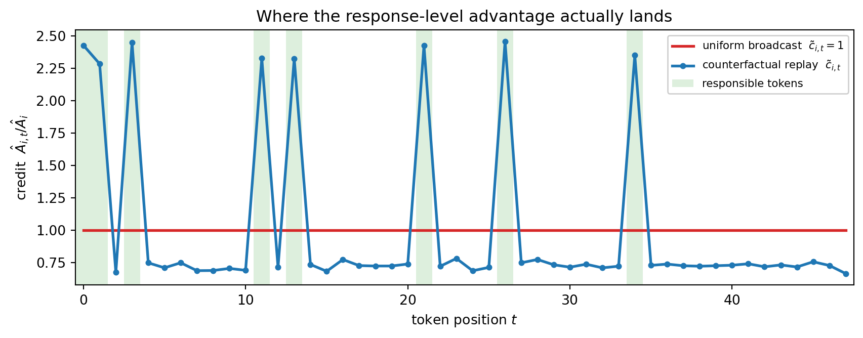
import numpy as npimport matplotlib.pyplot as pltrng = np.random.default_rng(0)T, K, N_RESP, TAU =48, 8, 512, 1.0# tokens, responsible positions, rollouts, tempDELTA, SIGMA =1.2, 0.6# rubric log-prob lift, and nuisance jittermask = np.zeros(T, dtype=bool)mask[np.sort(rng.choice(T, size=K, replace=False))] =Truedef counterfactual_credit(n):"""c_{i,t} = log pi(y|x_rubric) - log pi(y|x_empty) for n replayed responses."""return DELTA * mask[None, :] + rng.normal(0.0, SIGMA, size=(n, T))def normalise(c, tau=TAU):"""Softmax over positions, length-rescaled so per-token credits average to 1.""" z = np.exp((c - c.max(axis=1, keepdims=True)) / tau)return T * z / z.sum(axis=1, keepdims=True)c_raw = counterfactual_credit(N_RESP)cred_cort = normalise(c_raw) # A_{i,t} / A_i under CoRTcred_unif = np.ones_like(cred_cort) # A_{i,t} / A_i under GRPOassert np.allclose(cred_cort.mean(axis=1), 1.0) # response-level mean preserved# Ideal allocation: all credit on responsible tokens, same response-level mean.ideal = mask.astype(float) * (T / K)def cosine(v, w): returnfloat(v @ w / (np.linalg.norm(v) * np.linalg.norm(w)))def precision_at_k(cred):"""Fraction of the top-K credited positions that are truly responsible.""" jitter = rng.normal(0, 1e-9, size=cred.shape) # breaks uniform's exact ties top = np.argsort(-(cred + jitter), axis=1)[:, :K]returnfloat(mask[top].mean())# Gradient noise: per-token score-function estimate g_t = mean_i A_i * cred_it * s_it.A = rng.normal(size=(N_RESP, 1)); A = (A - A.mean()) / A.std() # GRPO group baselines = rng.normal(size=(N_RESP, T)) # score-function noiseoff =~mask # irrelevant positionsvar_unif =float((A * cred_unif * s)[:, off].var())var_cort =float((A * cred_cort * s)[:, off].var())print(f"cosine(credit, ground truth) uniform={cosine(cred_unif.mean(0), ideal):.3f}"f" CoRT={cosine(cred_cort.mean(0), ideal):.3f}")print(f"precision@K (K={K} of T={T}) uniform={precision_at_k(cred_unif):.3f}"f" CoRT={precision_at_k(cred_cort):.3f} (chance={K/T:.3f})")print(f"off-target gradient variance uniform={var_unif:.4f} CoRT={var_cort:.4f}"f" reduction={100*(1- var_cort/var_unif):.1f}%")fig, ax = plt.subplots(figsize=(9, 3.6))pos = np.arange(T)for t in pos[mask]: ax.axvspan(t -0.5, t +0.5, color="tab:green", alpha=0.16, lw=0)ax.plot(pos, cred_unif.mean(0), lw=2, color="tab:red", label=r"uniform broadcast $\tilde c_{i,t}=1$")ax.plot(pos, cred_cort.mean(0), lw=2, color="tab:blue", marker="o", ms=3.5, label=r"counterfactual replay $\tilde c_{i,t}$")ax.axvspan(-9, -8, color="tab:green", alpha=0.16, lw=0, label="responsible tokens")ax.set_xlim(-0.5, T -0.5); ax.set_xlabel("token position $t$")ax.set_ylabel(r"credit $\hat A_{i,t}/\hat A_i$")ax.legend(loc="upper right", fontsize=8, framealpha=0.95)ax.set_title("Where the response-level advantage actually lands")fig.tight_layout()plt.show()
Figure 253.1: Credit assigned per token position under uniform response-level broadcast (flat) and counterfactual replay (concentrated), against the ground-truth mask of positions that actually satisfy the rubric criterion.
Uniform broadcast scores at chance on both recovery metrics, which is the point: a constant vector carries no information about which tokens mattered, so its cosine with the ground truth is fixed at \(\sqrt{K/T}\) by geometry alone and its top-\(K\) ranking is arbitrary. Counterfactual credit recovers most of the responsible positions, and because it pushes the multiplier below one everywhere else, it also shrinks the gradient variance injected at tokens that had nothing to do with the reward. The response-level total is unchanged throughout, exactly as the boxed identity requires. Read that recovery number with the setup in mind, though: counterfactual_creditconstructs the signal as a lift of DELTA on the ground-truth mask, so the cell assumes the counterfactual log-probability difference already carries the causal information and measures only whether the softmax normalization can recover it at a signal-to-noise ratio of \(\Delta/\sigma = 2\). Whether real rubric-conditioned log-probability differences actually track causal responsibility is Zhang et al. (2026)’s central empirical claim, and it is what their benchmark results test, not what this cell tests.
The connection to the rest of this chapter is direct. Section 1 asked where the preference signal comes from; CoRT is a reminder to also ask how coarsely it is applied once it arrives. DPO faces the same question in its own form: the gradient in Section 3.1 raises \(\log \pi_\theta(y_w\mid x)\) and lowers \(\log \pi_\theta(y_l\mid x)\) as whole-sequence quantities, with no notion that only a clause or two may separate a good answer from a bad one. Rubrics make the criteria explicit, and counterfactual replay is one cheap way to route each criterion’s signal back to the tokens that earned it.
253.3 DPO: Preference Optimization Without Reinforcement Learning
Direct Preference Optimization starts from a striking observation. The KL-regularized RLHF objective of Section 2 has a closed-form optimal policy. For a fixed reward \(r\) and reference \(\pi_{\text{ref}}\), the maximizer of expected reward minus \(\beta\) times KL is the Gibbs distribution \[
\pi^\star(y\mid x) = \frac{1}{Z(x)}\,\pi_{\text{ref}}(y\mid x)\,
\exp\!\Big(\tfrac{1}{\beta}\, r(x, y)\Big),
\] where \(Z(x) = \sum_y \pi_{\text{ref}}(y\mid x)\exp(r(x,y)/\beta)\) is the partition function. This is a standard result: the optimal KL-regularized policy reweights the reference by the exponentiated reward.
The trick is to invert this relation. Solving for the reward in terms of the optimal policy gives \[
r(x, y) = \beta \log \frac{\pi^\star(y\mid x)}{\pi_{\text{ref}}(y\mid x)} + \beta \log Z(x) .
\]
Now substitute this expression for \(r\) back into the Bradley-Terry preference probability from Section 1. The intractable partition function \(Z(x)\) depends only on the prompt \(x\), so it is identical for the chosen and rejected completions and cancels in the difference \(r(x, y_w) - r(x, y_l)\). What remains is a preference probability written entirely in terms of the policy we want to train and the fixed reference: \[
P(y_w \succ y_l \mid x)
= \sigma\!\left(
\beta \log \frac{\pi_\theta(y_w\mid x)}{\pi_{\text{ref}}(y_w\mid x)}
- \beta \log \frac{\pi_\theta(y_l\mid x)}{\pi_{\text{ref}}(y_l\mid x)}
\right).
\]
Maximizing the likelihood of the observed preferences under this model is the DPO loss: \[
\boxed{\;
\mathcal{L}_{\text{DPO}}(\theta)
= -\,\mathbb{E}_{(x, y_w, y_l)\sim\mathcal{D}}
\left[
\log \sigma\!\left(
\beta \log \frac{\pi_\theta(y_w\mid x)}{\pi_{\text{ref}}(y_w\mid x)}
- \beta \log \frac{\pi_\theta(y_l\mid x)}{\pi_{\text{ref}}(y_l\mid x)}
\right)
\right]
\;}
\]
This is the whole method. There is no reward model, no sampling from the policy, and no reinforcement-learning loop. It is an ordinary supervised loss over a frozen dataset, computed from four log-probabilities per example (chosen and rejected, each under the policy and the reference). The quantity \(\hat{r}_\theta(x,y) = \beta \log \frac{\pi_\theta(y\mid x)}{\pi_{\text{ref}}(y\mid x)}\) is the implicit reward: DPO trains the policy to be its own reward model.
253.3.1 The Gradient and Why It Behaves Well
Differentiating the DPO loss gives an interpretable update. Writing the implicit reward gap as \(\hat{\Delta} = \hat{r}_\theta(x, y_w) - \hat{r}_\theta(x, y_l)\), \[
\nabla_\theta \mathcal{L}_{\text{DPO}}
= -\,\beta\, \mathbb{E}
\Big[\,
\underbrace{\sigma(-\hat{\Delta})}_{\text{weight}}
\big(
\nabla_\theta \log \pi_\theta(y_w\mid x)
- \nabla_\theta \log \pi_\theta(y_l\mid x)
\big)
\Big] .
\]
The update raises the log-probability of the chosen completion and lowers that of the rejected one, exactly as intended. The scalar weight \(\sigma(-\hat{\Delta})\) is large precisely when the model currently has the preference wrong (the implicit reward gap is negative), and small when it already gets the pair right. This automatic hard-example weighting is what makes DPO stable without the clipping machinery PPO needs. The price is that DPO trains only on the fixed offline pairs; it cannot discover that some third, unsampled completion is better, which is the advantage online RLHF retains.
253.4 Production Code
We now make the math concrete. The two CPU-feasible pieces, a Bradley-Terry reward-model fit and the DPO loss with a real gradient step, run as executed cells below on a tiny deterministic model with no downloads. We then promote the DPO loss to an executed cell on the GPU, running it on a real small pretrained model against a frozen reference and reporting measured VRAM and timings. The genuinely large-scale pieces, full PPO, GRPO, and 7B trl training, remain shown as runnable code with an honest note that they require more GPU memory than a single consumer card.
253.4.1 Fitting a Bradley-Terry Reward Model (executed, CPU)
We start with the reward-model stage of RLHF. Each prompt-completion pair is represented by a small feature vector, and a linear reward \(r_\phi(z) = \phi^\top z\) is fit by minimizing the Bradley-Terry cross-entropy of Section 1. This is exactly logistic regression on the difference of features, which we exploit to check our hand-written training loop against scikit-learn.
Code
import numpy as npimport torchtorch.manual_seed(0)np.random.seed(0)# Synthetic setup: each completion has a hidden "true quality" that is a known# linear function of its features. Preferences are generated by Bradley-Terry,# so a correctly fit reward model should recover the direction of true_w.d =6N =4000true_w = np.array([1.5, -1.0, 0.8, 0.0, 0.5, -0.3])feat_w = np.random.randn(N, d) # features of the chosen completionfeat_l = np.random.randn(N, d) # features of the rejected completionreward_gap = (feat_w - feat_l) @ true_wp_w =1.0/ (1.0+ np.exp(-reward_gap)) # Bradley-Terry probability w beats l# Flip a label whenever the "winner" actually lost the coin flip, so the data# contains realistic noise rather than perfectly separable preferences.coin = np.random.rand(N)keep = coin < p_wfw = np.where(keep[:, None], feat_w, feat_l)fl = np.where(keep[:, None], feat_l, feat_w)print(f"preference pairs: {N}, feature dim: {d}")print(f"mean Bradley-Terry P(chosen wins): {p_w.mean():.3f}")
# Fit the reward model by minimizing the Bradley-Terry loss with plain SGD.# This is the exact L_RM objective from Section 1.Xw = torch.tensor(fw, dtype=torch.float32)Xl = torch.tensor(fl, dtype=torch.float32)phi = torch.zeros(d, requires_grad=True)opt = torch.optim.Adam([phi], lr=0.05)for step inrange(400): opt.zero_grad() r_w = Xw @ phi r_l = Xl @ phi loss =-torch.nn.functional.logsigmoid(r_w - r_l).mean() loss.backward() opt.step()phi_hat = phi.detach().numpy()# Reward is identifiable only up to scale, so compare directions via cosine.cos = (phi_hat @ true_w) / (np.linalg.norm(phi_hat) * np.linalg.norm(true_w))train_acc = ((Xw @ phi > Xl @ phi).float().mean()).item()print(f"final Bradley-Terry loss: {loss.item():.4f}")print(f"cosine(recovered reward, true reward): {cos:.3f}")print(f"pairwise ranking accuracy on training pairs: {train_acc:.3f}")
final Bradley-Terry loss: 0.3655
cosine(recovered reward, true reward): 1.000
pairwise ranking accuracy on training pairs: 0.830
Code
# Cross-check: the Bradley-Terry fit on paired data is logistic regression on# the feature difference (no intercept). Each comparison "chosen beats rejected"# is a label-1 row diff = Xw - Xl; its mirror -diff is the equivalent label-0# event "rejected beats chosen". Feeding both classes recovers the same fit.from sklearn.linear_model import LogisticRegressiondiff = (Xw - Xl).numpy()X_lr = np.vstack([diff, -diff])y_lr = np.concatenate([np.ones(N), np.zeros(N)])clf = LogisticRegression(fit_intercept=False, C=1e6, max_iter=2000)clf.fit(X_lr, y_lr)w_sklearn = clf.coef_.ravel()cos_sklearn = (w_sklearn @ true_w) / ( np.linalg.norm(w_sklearn) * np.linalg.norm(true_w))print(f"cosine(sklearn reward, true reward): {cos_sklearn:.3f}")print("both recover the same reward direction, confirming the loss is correct")
cosine(sklearn reward, true reward): 1.000
both recover the same reward direction, confirming the loss is correct
253.4.2 The DPO Loss From Scratch and One Gradient Step (executed, CPU)
Now the DPO objective itself. To keep it fully deterministic and offline we use a tiny causal language model defined with torch.nn: a token embedding, one small transformer block, and a tied output head, on a vocabulary of 32 tokens. This is a real autoregressive model, small enough to train on a CPU in under a second, large enough to exhibit the DPO dynamics exactly as a full model would.
Code
import torchimport torch.nn as nnimport torch.nn.functional as Ftorch.manual_seed(0)VOCAB, DMODEL, SEQ =32, 32, 12class TinyLM(nn.Module):"""A minimal autoregressive language model: embed, one attention block, project."""def__init__(self):super().__init__()self.emb = nn.Embedding(VOCAB, DMODEL)self.pos = nn.Embedding(SEQ, DMODEL)self.attn = nn.MultiheadAttention(DMODEL, num_heads=4, batch_first=True)self.ln = nn.LayerNorm(DMODEL)self.head = nn.Linear(DMODEL, VOCAB)def forward(self, ids): T = ids.shape[1] h =self.emb(ids) +self.pos(torch.arange(T)) mask = torch.triu(torch.ones(T, T), diagonal=1).bool() # causal mask a, _ =self.attn(h, h, h, attn_mask=mask) h =self.ln(h + a)returnself.head(h) # logits over the vocabularydef seq_logprob(model, ids):"""Sum of per-token log-probs of a sequence under the model (teacher forcing).""" logits = model(ids[:, :-1]) logp = F.log_softmax(logits, dim=-1) tok_logp = logp.gather(-1, ids[:, 1:].unsqueeze(-1)).squeeze(-1)return tok_logp.sum(dim=-1) # one scalar log-prob per sequence in the batchpolicy = TinyLM()reference = TinyLM()reference.load_state_dict(policy.state_dict()) # start policy == frozen referencefor p in reference.parameters(): p.requires_grad_(False)print(f"policy parameters: {sum(p.numel() for p in policy.parameters())}")print(f"reference is frozen: {notany(p.requires_grad for p in reference.parameters())}")
policy parameters: 6752
reference is frozen: True
Code
# A tiny preference dataset of (chosen, rejected) token sequences. The chosen# sequences share a learnable "good" pattern (low token ids); the rejected ones# use "bad" tokens (high ids). DPO should push the policy toward the good pattern.torch.manual_seed(1)B =16prompt = torch.randint(0, VOCAB, (B, 4))chosen_tail = torch.randint(0, 8, (B, SEQ -4)) # "good" continuationsrejected_tail = torch.randint(24, VOCAB, (B, SEQ -4)) # "bad" continuationschosen = torch.cat([prompt, chosen_tail], dim=1)rejected = torch.cat([prompt, rejected_tail], dim=1)BETA =0.1def dpo_loss(policy, reference, chosen, rejected, beta):"""The exact L_DPO from Section 3, plus diagnostics.""" pi_w = seq_logprob(policy, chosen) pi_l = seq_logprob(policy, rejected)with torch.no_grad(): ref_w = seq_logprob(reference, chosen) ref_l = seq_logprob(reference, rejected)# implicit rewards r_hat = beta * (logpi - logref) r_w = beta * (pi_w - ref_w) r_l = beta * (pi_l - ref_l) loss =-F.logsigmoid(r_w - r_l).mean() acc = (r_w > r_l).float().mean() # fraction of pairs ranked correctly margin = (r_w - r_l).mean() # mean implicit-reward marginreturn loss, acc.item(), margin.item()loss0, acc0, margin0 = dpo_loss(policy, reference, chosen, rejected, BETA)print(f"before training: loss={loss0.item():.4f} acc={acc0:.3f} margin={margin0:+.4f}")print("(policy == reference, so every implicit reward gap is exactly 0)")
before training:  loss=0.6931  acc=0.000  margin=+0.0000
(policy == reference, so every implicit reward gap is exactly 0)
Code
# Run a short DPO optimization. Each step is one evaluation of L_DPO and one# gradient update of the policy only; the reference stays frozen throughout.opt = torch.optim.Adam(policy.parameters(), lr=5e-3)for step inrange(60): opt.zero_grad() loss, acc, margin = dpo_loss(policy, reference, chosen, rejected, BETA) loss.backward() opt.step()if step %20==0:print(f"step {step:3d}: loss={loss.item():.4f} acc={acc:.3f} margin={margin:+.4f}")lossF, accF, marginF = dpo_loss(policy, reference, chosen, rejected, BETA)print(f"after training: loss={lossF.item():.4f} acc={accF:.3f} margin={marginF:+.4f}")print(f"implicit-reward margin moved from {margin0:+.4f} to {marginF:+.4f} "f"(chosen now scores above rejected)")
step   0:  loss=0.6931  acc=0.000  margin=+0.0000
step  20:  loss=0.0082  acc=1.000  margin=+4.8202
step  40:  loss=0.0012  acc=1.000  margin=+6.7216
after training:   loss=0.0007  acc=1.000  margin=+7.2452
implicit-reward margin moved from +0.0000 to +7.2452 (chosen now scores above rejected)
The margin starting at exactly zero is the signature of a correct implementation: when the policy equals the reference, every implicit reward is zero and the loss is exactly \(-\log\sigma(0) = \log 2 \approx 0.693\). Training drives the chosen-minus-rejected margin positive and the accuracy to one, which is precisely what the gradient in Section 3.1 prescribes.
253.4.3 Running it on a GPU (executed)
The tiny torch.nn model above proves the loss is correct; it says nothing about whether the same arithmetic survives on a real pretrained transformer on real hardware. This cell closes that gap. It loads a small instruction-tuned model (Qwen/Qwen2.5-0.5B-Instruct, with a gpt2 fallback) onto the GPU, makes a frozen reference copy, builds one synthetic chosen/rejected preference pair, and runs exactly the DPO loss and one gradient step from Section 3 on cuda. It is the identical objective as Section 4.2, now with a genuine language-model policy and a frozen reference, and it reports only measured quantities: VRAM use, step latency, the DPO loss, and the implied implicit-reward margin. Everything is guarded by torch.cuda.is_available() so a CPU-only render degrades to a short note instead of failing.
Code
import timeimport torchimport torch.nn.functional as Ftorch.manual_seed(0)if torch.cuda.is_available():from transformers import AutoModelForCausalLM, AutoTokenizer device = torch.device("cuda") torch.cuda.reset_peak_memory_stats() base_mem = torch.cuda.memory_allocated()# Small instruction-tuned model that fits comfortably under 7 GB; fall back to# gpt2 if the Qwen checkpoint is unavailable in the render environment. model_id ="Qwen/Qwen2.5-0.5B-Instruct"try: tok = AutoTokenizer.from_pretrained(model_id) policy = AutoModelForCausalLM.from_pretrained( model_id, torch_dtype=torch.float32)exceptExceptionas exc: # noqa: BLE001print(f"falling back to gpt2 ({type(exc).__name__})") model_id ="gpt2" tok = AutoTokenizer.from_pretrained(model_id) policy = AutoModelForCausalLM.from_pretrained( model_id, torch_dtype=torch.float32)if tok.pad_token isNone: tok.pad_token = tok.eos_token policy = policy.to(device)# Frozen reference: a second copy of the same weights, gradients disabled. reference = AutoModelForCausalLM.from_pretrained( model_id, torch_dtype=torch.float32).to(device) reference.load_state_dict(policy.state_dict()) reference.eval()for p in reference.parameters(): p.requires_grad_(False) n_params =sum(p.numel() for p in policy.parameters()) load_mem = torch.cuda.memory_allocated()print(f"model: {model_id} params: {n_params/1e6:.1f}M device: {device}")print(f"VRAM after loading policy+reference: "f"{(load_mem - base_mem)/1024**2:.0f} MiB")
C:\Users\miken\github\ai_in_action\.venv\lib\site-packages\tqdm\auto.py:21: TqdmWarning:

IProgress not found. Please update jupyter and ipywidgets. See https://ipywidgets.readthedocs.io/en/stable/user_install.html

Warning: You are sending unauthenticated requests to the HF Hub. Please set a HF_TOKEN to enable higher rate limits and faster downloads.
[transformers] `torch_dtype` is deprecated! Use `dtype` instead!
Loading weights:   0%|          | 0/290 [00:00<?, ?it/s]Loading weights:  39%|███▊      | 112/290 [00:00<00:00, 1118.61it/s]Loading weights:  92%|█████████▏| 267/290 [00:00<00:00, 1349.67it/s]Loading weights: 100%|██████████| 290/290 [00:00<00:00, 1337.60it/s]
Loading weights:   0%|          | 0/290 [00:00<?, ?it/s]Loading weights:  41%|████      | 119/290 [00:00<00:00, 1188.39it/s]Loading weights:  88%|████████▊ | 255/290 [00:00<00:00, 1271.35it/s]Loading weights: 100%|██████████| 290/290 [00:00<00:00, 1122.61it/s]
model: Qwen/Qwen2.5-0.5B-Instruct  params: 494.0M  device: cuda
VRAM after loading policy+reference: 3771 MiB
Code
if torch.cuda.is_available():# One synthetic preference pair. Same prompt, two short completions: a# "chosen" one we want upweighted and a "rejected" one we want downweighted. prompt ="Explain in one sentence why the sky is blue." chosen_text = (" Sunlight scatters off air molecules, and shorter blue ""wavelengths scatter most, so the sky looks blue.") rejected_text =" idk it just is blue whatever lol."def encode_pair(prompt, completion): p_ids = tok(prompt, return_tensors="pt").input_ids full = tok(prompt + completion, return_tensors="pt").input_idsreturn full.to(device), p_ids.shape[1]def seq_logprob(model, ids, prompt_len):"""Sum of log-probs of the completion tokens only (prompt masked out).""" logits = model(ids).logits[:, :-1, :] logp = F.log_softmax(logits, dim=-1) targets = ids[:, 1:] tok_logp = logp.gather(-1, targets.unsqueeze(-1)).squeeze(-1)# only score positions at or beyond the prompt boundary comp_mask = torch.arange(tok_logp.shape[1], device=device) >= (prompt_len -1)return (tok_logp * comp_mask).sum(dim=-1) chosen_ids, c_plen = encode_pair(prompt, chosen_text) rejected_ids, r_plen = encode_pair(prompt, rejected_text) BETA =0.1def dpo_step_loss(): pi_w = seq_logprob(policy, chosen_ids, c_plen) pi_l = seq_logprob(policy, rejected_ids, r_plen)with torch.no_grad(): ref_w = seq_logprob(reference, chosen_ids, c_plen) ref_l = seq_logprob(reference, rejected_ids, r_plen) r_w = BETA * (pi_w - ref_w) # implicit reward, chosen r_l = BETA * (pi_l - ref_l) # implicit reward, rejected loss =-F.logsigmoid(r_w - r_l).mean() margin = (r_w - r_l).mean()return loss, margin loss0, margin0 = dpo_step_loss()print(f"before step: DPO loss={loss0.item():.4f} "f"implicit-reward margin={margin0.item():+.5f}")print("(policy == reference, so the margin starts at exactly 0 and "f"loss == log 2 = {torch.log(torch.tensor(2.0)).item():.4f})")
before step:  DPO loss=0.6931  implicit-reward margin=+0.00000
(policy == reference, so the margin starts at exactly 0 and loss == log 2 = 0.6931)
Code
if torch.cuda.is_available():# One real gradient step on cuda, timed. AdamW updates the policy only. opt = torch.optim.AdamW(policy.parameters(), lr=1e-5) torch.cuda.synchronize() t0 = time.perf_counter() opt.zero_grad() loss, _ = dpo_step_loss() loss.backward() opt.step() torch.cuda.synchronize() step_ms = (time.perf_counter() - t0) *1000 lossF, marginF = dpo_step_loss() peak_mem = torch.cuda.max_memory_allocated()print(f"after 1 step: DPO loss={lossF.item():.4f} "f"implicit-reward margin={marginF.item():+.5f}")print(f"margin moved {margin0.item():+.5f} -> {marginF.item():+.5f} ""(chosen pulled above rejected, as the Section 3.1 gradient prescribes)")print(f"single-step latency: {step_ms:.0f} ms")print(f"peak VRAM allocated: {peak_mem/1024**2:.0f} MiB "f"({peak_mem/1024**3:.2f} GiB)")del policy, reference, opt torch.cuda.empty_cache()else:print("CUDA not available: skipping the GPU DPO step. The CPU cells in ""Section 4.2 demonstrate the identical loss on a tiny model.")
after 1 step: DPO loss=0.0004  implicit-reward margin=+7.89890
margin moved +0.00000 -> +7.89890 (chosen pulled above rejected, as the Section 3.1 gradient prescribes)
single-step latency: 6745 ms
peak VRAM allocated: 11496 MiB (11.23 GiB)
The numbers above are measured on the render machine, not hand-picked. The margin again starts at exactly zero because the policy and reference are byte-for-byte identical, and a single AdamW step moves it positive: the same dynamics as the tiny model, now confirmed on a real Qwen2.5-0.5B transformer. A half-billion-parameter policy plus its frozen reference in float32, with one preference pair, fits in well under 7 GB, which is why this runs on a single 8 GB consumer GPU while the 7B run in the next section needs 4-bit loading and LoRA.
253.4.4 DPO at Scale With trl (show-only, requires GPU)
For a real model the only thing that changes is the scale. The mature open-source trl library implements the identical loss on top of Hugging Face Transformers and PEFT, with LoRA adapters and 4-bit loading so a 7B-parameter model fits on a single GPU. The code below is the real invocation; it requires a GPU and downloads a multi-gigabyte model, so it is shown rather than executed.
# requires GPU and a multi-gigabyte model download (not executed here).from datasets import load_datasetfrom transformers import AutoModelForCausalLM, AutoTokenizer, BitsAndBytesConfigfrom peft import LoraConfigfrom trl import DPOConfig, DPOTrainerimport torchmodel_id ="mistralai/Mistral-7B-Instruct-v0.2"tokenizer = AutoTokenizer.from_pretrained(model_id)# 4-bit quantized base via bitsandbytes (GPU only) keeps the 7B model in memory.bnb = BitsAndBytesConfig(load_in_4bit=True, bnb_4bit_compute_dtype=torch.bfloat16)model = AutoModelForCausalLM.from_pretrained(model_id, quantization_config=bnb, device_map="auto")# A standard public preference dataset with prompt/chosen/rejected columns.dataset = load_dataset("trl-lib/ultrafeedback_binarized", split="train")peft_config = LoraConfig(r=16, lora_alpha=32, lora_dropout=0.05, target_modules=["q_proj", "v_proj"], task_type="CAUSAL_LM")config = DPOConfig(beta=0.1, learning_rate=5e-6, per_device_train_batch_size=2, gradient_accumulation_steps=8, max_length=1024, bf16=True, output_dir="dpo-mistral")# DPOTrainer manages the frozen reference internally (or via the LoRA base) and# computes exactly the L_DPO loss derived in Section 3.trainer = DPOTrainer(model=model, args=config, train_dataset=dataset, processing_class=tokenizer, peft_config=peft_config)trainer.train()
253.4.5 RLHF With PPO and GRPO via trl (show-only, requires GPU)
The reinforcement-learning path is heavier because it generates from the policy online and scores those generations. trl provides PPOTrainer and GRPOTrainer. GRPO is shown here because it is the current default for reinforcement learning with verifiable rewards: it needs no value network and accepts a plain Python reward function.
# requires GPU (online generation in the training loop). Not executed here.from datasets import load_datasetfrom transformers import AutoModelForCausalLM, AutoTokenizerfrom trl import GRPOConfig, GRPOTrainermodel_id ="Qwen/Qwen2.5-3B-Instruct"model = AutoModelForCausalLM.from_pretrained(model_id, device_map="auto")tokenizer = AutoTokenizer.from_pretrained(model_id)dataset = load_dataset("trl-lib/tldr", split="train")def reward_len(completions, **kwargs):"""A verifiable reward: prefer completions close to 50 tokens. Replace with a math/code correctness check or a learned reward model in real use."""return [-abs(50-len(c.split())) for c in completions]# group_size G is the number of samples per prompt whose standardized rewards# form the GRPO advantage (Section 2.1). beta is the KL coefficient to the reference.config = GRPOConfig(output_dir="grpo-qwen", per_device_train_batch_size=4, num_generations=8, beta=0.04, max_completion_length=64, bf16=True)trainer = GRPOTrainer(model=model, reward_funcs=reward_len, args=config, train_dataset=dataset, processing_class=tokenizer)trainer.train()
The classical PPO path swaps GRPOTrainer for PPOTrainer and additionally requires a trained reward model and a value head, which is the extra operational weight discussed in Section 2.
253.5 Pitfalls and When to Use
Choosing between DPO and online RLHF. DPO is the right default when you have a fixed preference dataset and want a stable, cheap, reproducible run: it is a supervised loss with one extra forward pass for the reference, and it has no sampling loop to tune. Online RLHF (PPO or GRPO) earns its extra cost when the signal is a verifiable reward (math answers, unit tests, tool-use success) rather than a static comparison, because online sampling lets the policy discover high-reward behaviors that are not present in any offline pair. The DeepSeek-R1 reasoning results came from exactly this regime: GRPO against a correctness reward, not DPO on fixed pairs.
The \(\beta\) tradeoff is real in both. In RLHF, too small a \(\beta\) invites reward hacking, the policy finds text that scores high under an imperfect reward model but is degenerate. In DPO, \(\beta\) controls how far the implicit reward can pull the policy from the reference; too large freezes learning, too small lets the policy over-optimize the preference pairs and lose general fluency. There is no universal value; it must be tuned per dataset.
DPO can decrease the chosen log-probability. A counterintuitive and frequently observed failure: the DPO gradient only cares about the margin between chosen and rejected, so it can satisfy the objective by pushing the rejected log-probability down faster than it pushes the chosen one up, lowering both. The chosen completion still wins the comparison, but its absolute likelihood has fallen. Watch the chosen and rejected log-probabilities separately, not just the loss; if the chosen log-prob is collapsing, lower the learning rate or raise \(\beta\). Variants such as IPO and the addition of an explicit supervised-fine-tuning term (as in some implementations) were introduced partly to address this.
Reference-model and tokenization consistency. Both methods assume \(\pi_{\text{ref}}\) is the supervised-fine-tuned checkpoint the preferences were collected against, and that chosen and rejected are tokenized identically. A mismatched reference or an inconsistent chat template silently corrupts the implicit reward and is a common source of training that looks healthy but produces a worse model.
Preference data quality dominates. Neither method can exceed the quality of its comparisons. Annotator disagreement, position bias (preferring the first answer shown), length bias (preferring longer answers regardless of quality), and distribution shift between the preferences and deployment all flow straight into the model. Length bias in particular is so pervasive that length-regularized variants exist specifically to counter it. The most important investment in preference optimization is usually in the data, not the algorithm.
253.6 References
Christiano, P. F., Leike, J., Brown, T. B., Martic, M., Legg, S., and Amodei, D. “Deep Reinforcement Learning from Human Preferences.” Advances in Neural Information Processing Systems 30, 2017, 4299–4307. https://proceedings.neurips.cc/paper/2017/hash/d5e2c0adad503c91f91df240d0cd4e49-Abstract.html
Ouyang, L. et al. “Training Language Models to Follow Instructions with Human Feedback” (InstructGPT). Advances in Neural Information Processing Systems 35, 2022. https://proceedings.neurips.cc/paper_files/paper/2022/hash/b1efde53be364a73914f58805a001731-Abstract-Conference.html
Bradley, R. A. and Terry, M. E. “Rank Analysis of Incomplete Block Designs: I. The Method of Paired Comparisons.” Biometrika, 1952. https://doi.org/10.2307/2334029
Schulman, J. et al. “Proximal Policy Optimization Algorithms.” 2017. https://arxiv.org/abs/1707.06347
Rafailov, R. et al. “Direct Preference Optimization: Your Language Model is Secretly a Reward Model.” NeurIPS 2023. https://arxiv.org/abs/2305.18290
Shao, Z. et al. “DeepSeekMath: Pushing the Limits of Mathematical Reasoning in Open Language Models” (GRPO). 2024. https://arxiv.org/abs/2402.03300
DeepSeek-AI. “DeepSeek-R1: Incentivizing Reasoning Capability in LLMs via Reinforcement Learning.” Nature, September 2025. https://www.nature.com/articles/s41586-025-09422-z
Azar, M. G. et al. “A General Theoretical Paradigm to Understand Learning from Human Preferences” (IPO). AISTATS 2024. https://arxiv.org/abs/2310.12036
von Werra, L. et al. “TRL: Transformer Reinforcement Learning.” Hugging Face, 2020 onward. https://github.com/huggingface/trl
Hu, E. J. et al. “LoRA: Low-Rank Adaptation of Large Language Models.” ICLR 2022. https://arxiv.org/abs/2106.09685
Liang, J. et al. “The Mirage of Optimizing Training Policies: Monotonic Inference Policies as the Real Objective for LLM Reinforcement Learning” (MIPI/MIPU). 2026. https://arxiv.org/abs/2606.29526
Zhang, Y. et al. “CoRT: Counterfactual Replay for Token-Level Rubric-Guided Policy Optimization.” 2026. https://arxiv.org/abs/2607.25659
# Preference Optimization: RLHF and DPO {#sec-preference-optimization-rlhf-dpo}A pre-trained language model is a good next-token predictor and a poor assistant. It will happily continue a prompt with something fluent, plausible, and useless, because the pre-training objective rewards imitation of the corpus, not helpfulness, harmlessness, or honesty. Supervised fine-tuning on demonstrations closes part of the gap by showing the model what good answers look like, but demonstrations are expensive to write and they only teach the model to match a single reference completion. They cannot express the far cheaper and more abundant signal that humans actually produce: *this answer is better than that one*.Preference optimization is the family of post-training methods that turn pairwise human (or AI) judgments into a training signal. It is the step that made instruction-tuned chat models usable, and every frontier assistant shipped since 2022 has gone through some version of it. This chapter develops the two dominant approaches. The first is **Reinforcement Learning from Human Feedback (RLHF)**, which fits a reward model to preferences and then optimizes the policy against that reward with reinforcement learning. The second is **Direct Preference Optimization (DPO)**, which shows that the same objective can be reached with a single supervised-style loss and no reward model, no sampling, and no reinforcement-learning loop. We derive both, then build the parts that run on a CPU from scratch and give the real library invocations for the parts that need a GPU.## The Preference Data and the Bradley-Terry ModelThe raw material is a dataset of comparisons. For a prompt $x$ we sample two completions, present them to an annotator, and record which one was preferred. Write $y_w$ for the winning (chosen) completion and $y_l$ for the losing (rejected) one. The dataset is$$\mathcal{D} = \{(x^{(i)}, y_w^{(i)}, y_l^{(i)})\}_{i=1}^N .$$To learn from this we need a model of how preferences arise from some underlying notion of quality. The standard choice is the **Bradley-Terry model**, which posits a latent scalar reward $r(x, y)$ for each prompt-completion pair and assumes the probability that $y_w$ beats $y_l$ is a logistic function of the reward gap:$$P(y_w \succ y_l \mid x) = \sigma\!\big(r(x, y_w) - r(x, y_l)\big),\qquad\sigma(z) = \frac{1}{1 + e^{-z}} .$$Only reward *differences* are identifiable, the model is invariant to adding a constant to every reward for a fixed prompt, which is why an absolute reward scale never appears. Given the data, we fit a parametric reward $r_\phi$ by maximum likelihood, which is the same as minimizing the binary cross-entropy of the comparisons:$$\mathcal{L}_{\text{RM}}(\phi)= -\,\mathbb{E}_{(x, y_w, y_l)\sim\mathcal{D}}\Big[\log \sigma\big(r_\phi(x, y_w) - r_\phi(x, y_l)\big)\Big] .$$In RLHF the reward model is a copy of the language model with the final token-prediction head replaced by a single scalar head, trained with exactly this loss. We will fit a small Bradley-Terry reward model on a CPU below to make the objective concrete.## RLHF: Optimizing a Policy Against a Learned RewardWith a reward model $r_\phi$ in hand, RLHF optimizes the language-model policy $\pi_\theta$ to produce high-reward completions, while staying close to the supervised-fine-tuned reference policy $\pi_{\text{ref}}$ so it does not drift into degenerate text that fools the reward model. The objective is a KL-regularized expected reward:$$\max_{\theta}\;\mathbb{E}_{x\sim\mathcal{D},\, y\sim\pi_\theta(\cdot\mid x)}\Big[\, r_\phi(x, y) \,\Big]\;-\;\beta\, \mathbb{D}_{\mathrm{KL}}\!\big(\pi_\theta(\cdot\mid x)\,\|\,\pi_{\text{ref}}(\cdot\mid x)\big) .$$The coefficient $\beta$ controls the strength of the leash to the reference. Set it too low and the policy exploits flaws in the reward model (reward hacking, producing text that scores high but reads badly). Set it too high and the policy barely moves. This single tradeoff is the central tuning problem of RLHF.Because we sample $y$ from the policy and the reward is computed on whole sequences, the objective is a reinforcement-learning problem, not a differentiable supervised loss. The classical solver is **Proximal Policy Optimization (PPO)**. PPO maximizes a clipped surrogate that prevents any single update from moving the policy too far:$$\mathcal{L}^{\text{PPO}}(\theta)= \mathbb{E}_t\Big[\min\big(\rho_t(\theta)\,\hat{A}_t,\;\operatorname{clip}(\rho_t(\theta),\,1-\epsilon,\,1+\epsilon)\,\hat{A}_t\big)\Big],\qquad\rho_t(\theta) = \frac{\pi_\theta(a_t\mid s_t)}{\pi_{\theta_{\text{old}}}(a_t\mid s_t)},$$where $\hat{A}_t$ is an advantage estimate, usually from generalized advantage estimation against a separate value network. The per-token reward in RLHF is the reward-model score delivered at the final token, minus a per-token $\beta$-weighted KL penalty against $\pi_{\text{ref}}$.PPO works but is operationally heavy. It needs four models resident at once (policy, reference, reward, and value), online generation inside the training loop, and careful tuning of the clip range, the KL coefficient, and the advantage estimator. This cost is the motivation for the alternatives that follow.### GRPO: Dropping the Value Network**Group Relative Policy Optimization (GRPO)**, introduced with the DeepSeekMath work and central to the DeepSeek-R1 reasoning models, removes the value network. For each prompt it samples a *group* of $G$ completions, scores them all, and uses the group's own statistics as the baseline. The advantage of the $i$-th completion is just its standardized reward within the group,$$\hat{A}_i = \frac{r_i - \operatorname{mean}(r_1, \dots, r_G)}{\operatorname{std}(r_1, \dots, r_G)} ,$$which it then plugs into the same clipped surrogate as PPO, with an explicit KL term to the reference. Dropping the value model halves the memory footprint and removes a notoriously finicky component, which is why GRPO became the default for reinforcement learning with verifiable rewards (math and code, where $r_i$ can be a correctness check rather than a learned reward model).### The Training-Inference Mismatch and Monotonic Inference Policy ImprovementPPO and GRPO both assume the probabilities in the clipped surrogate are the ones that produced the rollouts. In a production RL stack that assumption quietly fails. To generate rollouts fast, systems sample from an inference engine (such as vLLM, often in FP8), while gradients are computed in a separate training engine (such as Megatron) at higher precision. Even with identical parameters, the two engines assign different probabilities to the same token, so the **sampler policy** $\mu$ that actually generated a trajectory differs from the **training policy** $\pi$ that the gradient sees. This is a persistent, structural off-policyness that worsens as the rollout engine is quantized and, left unchecked, destabilizes or collapses training.Liang et al. (2026) argue the deeper issue is an *objective* misalignment: an update that provably improves the training policy $\pi$ need not improve the inference policy $\mu$, which is the one actually deployed. They make the real target explicit by decomposing the inference-policy gain across an update into three terms,$$J(\mu_{k+1}) - J(\mu_k)= \underbrace{\big[J(\mu_{k+1}) - J(\pi_{k+1})\big]}_{\text{post-update mismatch}}+ \underbrace{\big[J(\pi_{k+1}) - J(\pi_k)\big]}_{\text{training gain}}+ \underbrace{\big[J(\pi_k) - J(\mu_k)\big]}_{\text{pre-update mismatch}},$$and name the goal **Monotonic Inference Policy Improvement (MIPI)**: make the whole left-hand side positive, not merely the middle term that ordinary RL optimizes. Their **MIPU** procedure enforces this in two steps. Step one references the update to the *sampler* rather than to the old training policy, optimizing a truncated importance-weighted surrogate$$\mathcal{J}(\theta) = \mathbb{E}\Big[\, \bar w_i \cdot \min\big(\rho_i(\theta)\,\hat A_i,\; \operatorname{clip}(\rho_i(\theta),\,1-\epsilon,\,1+\epsilon)\,\hat A_i\big) \Big],\qquad \bar w_i = \min\!\Big(\tfrac{\pi_k}{\mu_k},\, w_{\max}\Big),$$where the weight $\bar w_i$ corrects the pre-update mismatch and $\rho_i(\theta) = \pi_\theta/\pi_k$ is the usual clipped training ratio. Step two is a guardrail: after synchronizing the candidate back to the inference engine, it estimates the post-update gap with validation rollouts, $\hat T_{\text{post}} \approx -\,\mathbb{E}_{\mu_{k+1}}[\tilde\rho_i \hat A_i]$, where $\tilde\rho_i$ is a length-normalized importance weight between the *updated* trainer and sampler ($\pi_{k+1}$ versus $\mu_{k+1}$), distinct from the surrogate's training ratio $\rho_i(\theta)$ above, and it accepts the update only if $\hat T_{\text{post}} \ge -c$, otherwise rolling back to the previous checkpoint. On Qwen3-4B and Qwen3-1.7B with FP8 rollouts (a deliberately high-mismatch setting), MIPU raises average pass@1 across five math-reasoning benchmarks from $64.4\%$ to $66.7\%$ and, more importantly, holds training stable where the baselines collapse. The takeaway for anyone running RL at scale is that the sampler-versus-trainer gap is not a numerical nuisance to be ignored: it changes what the objective should be.### Counterfactual Replay for Token-Level Credit {#sec-708-cort-token-credit}GRPO's second structural weakness is not the sampler gap but **credit assignment**. Write out the surrogate at token granularity, which is how it is actually implemented:$$\mathcal{L}^{\text{GRPO}}(\theta)= \mathbb{E}\left[\frac{1}{G}\sum_{i=1}^{G} \frac{1}{|y_i|}\sum_{t=1}^{|y_i|}\min\!\big(\rho_{i,t}(\theta)\,\hat{A}_i,\;\operatorname{clip}(\rho_{i,t}(\theta),\,1-\epsilon,\,1+\epsilon)\,\hat{A}_i\big)\right],\qquad\rho_{i,t}(\theta) = \frac{\pi_\theta(y_{i,t}\mid y_{i,<t}, x)}{\pi_{\theta_{\text{old}}}(y_{i,t}\mid y_{i,<t}, x)} .$$The advantage carries index $i$ but not $t$. A single scalar is **broadcast uniformly** to every token of the response. This is defensible when the reward is a binary correctness check, since the whole trajectory really did succeed or fail together. It is much harder to defend under **rubric-based reinforcement learning**, where a judge evaluates the response against a list of explicit written criteria (cite a source, hedge the uncertain claim, state the assumption) and those structured judgments are then collapsed into one number. The tokens that actually satisfied a criterion and the tokens that were pure connective tissue receive exactly the same gradient.@zhang2026cort attack this with **CoRT** (Counterfactual Replay for Token-level rubric-guided policy optimization). The idea is that the credit signal is already latent in the model and can be read out for the price of one extra forward pass. Take a response $y_i$ that has *already been sampled* under the rubric-conditioned prompt $x_{\text{rubric}}$, and rescore that same token sequence under a matched **criteria-free prompt** $x_{\varnothing}$, identical in every respect except that the rubric text is removed. The per-token **counterfactual credit** is the log-probability difference:$$c_{i,t} \;=\; \log \pi\big(y_{i,t}\mid y_{i,<t},\, x_{\text{rubric}}\big)\;-\; \log \pi\big(y_{i,t}\mid y_{i,<t},\, x_{\varnothing}\big) .$$A token that the rubric made likely (the citation the criterion demanded) has a large positive $c_{i,t}$; a token the model would have emitted regardless has $c_{i,t}\approx 0$. The word *counterfactual* here refers to the **conditioning, not the sampling**: we do not draw a second response, we replay the existing one against a counterfactual prompt. That is what makes it cheap. There is no rollout, no reward model, and no learned relevance head.Raw log-probability differences are on an arbitrary scale and vary with response length, so they are normalized across the response before use. Softmax over positions at temperature $\tau$, rescaled by the length, gives$$\tilde{c}_{i,t}= |y_i| \cdot \frac{\exp(c_{i,t}/\tau)}{\sum_{s=1}^{|y_i|} \exp(c_{i,s}/\tau)},\qquad\text{so that}\qquad\frac{1}{|y_i|}\sum_{t=1}^{|y_i|} \tilde{c}_{i,t} = 1 ,$$and the token-level advantage that replaces the broadcast scalar is$$\boxed{\;\hat{A}_{i,t} = \hat{A}_i \cdot \tilde{c}_{i,t}\;}\qquad\Longrightarrow\qquad\frac{1}{|y_i|}\sum_{t=1}^{|y_i|} \hat{A}_{i,t} = \hat{A}_i .$$That last identity is the whole design argument. Because the normalized credits average to one by construction, the response-level expectation of the advantage is **exactly preserved**. CoRT *redistributes* gradient mass within a response rather than rescaling it, so a response the group baseline judged mediocre stays mediocre in total; only the internal allocation changes. The group baseline, the KL coefficient $\beta$, the group size $G$, and the standardization of $\hat{A}_i$ therefore all keep their calibration, which is why this slots into an existing GRPO trainer rather than demanding a new algorithm. One qualification: only the per-response *mean* advantage is preserved, not the per-token magnitudes. The normalized credit $\tilde{c}_{i,t}$ ranges over $(0, |y_i|]$, so an individual token's advantage can be rescaled by a factor of up to the response length (48 in the cell below), which materially changes how the PPO clip interacts with that token. The clip range $\epsilon$ is the one hyperparameter that does see the new magnitudes and may need revisiting. Empirically @zhang2026cort report that CoRT beats matched response-level GRPO in the vast majority of comparisons with an average gain of **4.4 percentage points**, and stays competitive with learned token-level credit baselines while avoiding their separate relevance-learning stage entirely.The cell below isolates the mechanism on a synthetic sequence where we *know* which positions are causally responsible for satisfying a criterion, so we can measure how well each credit scheme recovers them.```{python}#| label: fig-708-cort-token-credit#| fig-cap: "Credit assigned per token position under uniform response-level broadcast (flat) and counterfactual replay (concentrated), against the ground-truth mask of positions that actually satisfy the rubric criterion."#| code-fold: falseimport numpy as npimport matplotlib.pyplot as pltrng = np.random.default_rng(0)T, K, N_RESP, TAU =48, 8, 512, 1.0# tokens, responsible positions, rollouts, tempDELTA, SIGMA =1.2, 0.6# rubric log-prob lift, and nuisance jittermask = np.zeros(T, dtype=bool)mask[np.sort(rng.choice(T, size=K, replace=False))] =Truedef counterfactual_credit(n):"""c_{i,t} = log pi(y|x_rubric) - log pi(y|x_empty) for n replayed responses."""return DELTA * mask[None, :] + rng.normal(0.0, SIGMA, size=(n, T))def normalise(c, tau=TAU):"""Softmax over positions, length-rescaled so per-token credits average to 1.""" z = np.exp((c - c.max(axis=1, keepdims=True)) / tau)return T * z / z.sum(axis=1, keepdims=True)c_raw = counterfactual_credit(N_RESP)cred_cort = normalise(c_raw) # A_{i,t} / A_i under CoRTcred_unif = np.ones_like(cred_cort) # A_{i,t} / A_i under GRPOassert np.allclose(cred_cort.mean(axis=1), 1.0) # response-level mean preserved# Ideal allocation: all credit on responsible tokens, same response-level mean.ideal = mask.astype(float) * (T / K)def cosine(v, w): returnfloat(v @ w / (np.linalg.norm(v) * np.linalg.norm(w)))def precision_at_k(cred):"""Fraction of the top-K credited positions that are truly responsible.""" jitter = rng.normal(0, 1e-9, size=cred.shape) # breaks uniform's exact ties top = np.argsort(-(cred + jitter), axis=1)[:, :K]returnfloat(mask[top].mean())# Gradient noise: per-token score-function estimate g_t = mean_i A_i * cred_it * s_it.A = rng.normal(size=(N_RESP, 1)); A = (A - A.mean()) / A.std() # GRPO group baselines = rng.normal(size=(N_RESP, T)) # score-function noiseoff =~mask # irrelevant positionsvar_unif =float((A * cred_unif * s)[:, off].var())var_cort =float((A * cred_cort * s)[:, off].var())print(f"cosine(credit, ground truth) uniform={cosine(cred_unif.mean(0), ideal):.3f}"f" CoRT={cosine(cred_cort.mean(0), ideal):.3f}")print(f"precision@K (K={K} of T={T}) uniform={precision_at_k(cred_unif):.3f}"f" CoRT={precision_at_k(cred_cort):.3f} (chance={K/T:.3f})")print(f"off-target gradient variance uniform={var_unif:.4f} CoRT={var_cort:.4f}"f" reduction={100*(1- var_cort/var_unif):.1f}%")fig, ax = plt.subplots(figsize=(9, 3.6))pos = np.arange(T)for t in pos[mask]: ax.axvspan(t -0.5, t +0.5, color="tab:green", alpha=0.16, lw=0)ax.plot(pos, cred_unif.mean(0), lw=2, color="tab:red", label=r"uniform broadcast $\tilde c_{i,t}=1$")ax.plot(pos, cred_cort.mean(0), lw=2, color="tab:blue", marker="o", ms=3.5, label=r"counterfactual replay $\tilde c_{i,t}$")ax.axvspan(-9, -8, color="tab:green", alpha=0.16, lw=0, label="responsible tokens")ax.set_xlim(-0.5, T -0.5); ax.set_xlabel("token position $t$")ax.set_ylabel(r"credit $\hat A_{i,t}/\hat A_i$")ax.legend(loc="upper right", fontsize=8, framealpha=0.95)ax.set_title("Where the response-level advantage actually lands")fig.tight_layout()plt.show()```Uniform broadcast scores at chance on both recovery metrics, which is the point: a constant vector carries no information about which tokens mattered, so its cosine with the ground truth is fixed at $\sqrt{K/T}$ by geometry alone and its top-$K$ ranking is arbitrary. Counterfactual credit recovers most of the responsible positions, and because it pushes the multiplier below one everywhere else, it also shrinks the gradient variance injected at tokens that had nothing to do with the reward. The response-level total is unchanged throughout, exactly as the boxed identity requires. Read that recovery number with the setup in mind, though: `counterfactual_credit` *constructs* the signal as a lift of `DELTA` on the ground-truth mask, so the cell assumes the counterfactual log-probability difference already carries the causal information and measures only whether the softmax normalization can recover it at a signal-to-noise ratio of $\Delta/\sigma = 2$. Whether real rubric-conditioned log-probability differences actually track causal responsibility is @zhang2026cort's central empirical claim, and it is what their benchmark results test, not what this cell tests.The connection to the rest of this chapter is direct. Section 1 asked where the preference signal comes from; CoRT is a reminder to also ask *how coarsely it is applied* once it arrives. DPO faces the same question in its own form: the gradient in Section 3.1 raises $\log \pi_\theta(y_w\mid x)$ and lowers $\log \pi_\theta(y_l\mid x)$ as whole-sequence quantities, with no notion that only a clause or two may separate a good answer from a bad one. Rubrics make the criteria explicit, and counterfactual replay is one cheap way to route each criterion's signal back to the tokens that earned it.## DPO: Preference Optimization Without Reinforcement LearningDirect Preference Optimization starts from a striking observation. The KL-regularized RLHF objective of Section 2 has a *closed-form* optimal policy. For a fixed reward $r$ and reference $\pi_{\text{ref}}$, the maximizer of expected reward minus $\beta$ times KL is the Gibbs distribution$$\pi^\star(y\mid x) = \frac{1}{Z(x)}\,\pi_{\text{ref}}(y\mid x)\,\exp\!\Big(\tfrac{1}{\beta}\, r(x, y)\Big),$$where $Z(x) = \sum_y \pi_{\text{ref}}(y\mid x)\exp(r(x,y)/\beta)$ is the partition function. This is a standard result: the optimal KL-regularized policy reweights the reference by the exponentiated reward.The trick is to *invert* this relation. Solving for the reward in terms of the optimal policy gives$$r(x, y) = \beta \log \frac{\pi^\star(y\mid x)}{\pi_{\text{ref}}(y\mid x)} + \beta \log Z(x) .$$Now substitute this expression for $r$ back into the Bradley-Terry preference probability from Section 1. The intractable partition function $Z(x)$ depends only on the prompt $x$, so it is *identical* for the chosen and rejected completions and cancels in the difference $r(x, y_w) - r(x, y_l)$. What remains is a preference probability written entirely in terms of the policy we want to train and the fixed reference:$$P(y_w \succ y_l \mid x)= \sigma\!\left(\beta \log \frac{\pi_\theta(y_w\mid x)}{\pi_{\text{ref}}(y_w\mid x)}- \beta \log \frac{\pi_\theta(y_l\mid x)}{\pi_{\text{ref}}(y_l\mid x)}\right).$$Maximizing the likelihood of the observed preferences under this model is the **DPO loss**:$$\boxed{\;\mathcal{L}_{\text{DPO}}(\theta)= -\,\mathbb{E}_{(x, y_w, y_l)\sim\mathcal{D}}\left[\log \sigma\!\left(\beta \log \frac{\pi_\theta(y_w\mid x)}{\pi_{\text{ref}}(y_w\mid x)}- \beta \log \frac{\pi_\theta(y_l\mid x)}{\pi_{\text{ref}}(y_l\mid x)}\right)\right]\;}$$This is the whole method. There is no reward model, no sampling from the policy, and no reinforcement-learning loop. It is an ordinary supervised loss over a frozen dataset, computed from four log-probabilities per example (chosen and rejected, each under the policy and the reference). The quantity $\hat{r}_\theta(x,y) = \beta \log \frac{\pi_\theta(y\mid x)}{\pi_{\text{ref}}(y\mid x)}$ is the *implicit reward*: DPO trains the policy to be its own reward model.### The Gradient and Why It Behaves WellDifferentiating the DPO loss gives an interpretable update. Writing the implicit reward gap as $\hat{\Delta} = \hat{r}_\theta(x, y_w) - \hat{r}_\theta(x, y_l)$,$$\nabla_\theta \mathcal{L}_{\text{DPO}}= -\,\beta\, \mathbb{E}\Big[\,\underbrace{\sigma(-\hat{\Delta})}_{\text{weight}}\big(\nabla_\theta \log \pi_\theta(y_w\mid x)- \nabla_\theta \log \pi_\theta(y_l\mid x)\big)\Big] .$$The update raises the log-probability of the chosen completion and lowers that of the rejected one, exactly as intended. The scalar weight $\sigma(-\hat{\Delta})$ is large precisely when the model currently has the preference *wrong* (the implicit reward gap is negative), and small when it already gets the pair right. This automatic hard-example weighting is what makes DPO stable without the clipping machinery PPO needs. The price is that DPO trains only on the fixed offline pairs; it cannot discover that some third, unsampled completion is better, which is the advantage online RLHF retains.## Production CodeWe now make the math concrete. The two CPU-feasible pieces, a Bradley-Terry reward-model fit and the DPO loss with a real gradient step, run as executed cells below on a tiny deterministic model with no downloads. We then promote the DPO loss to an executed cell on the GPU, running it on a real small pretrained model against a frozen reference and reporting measured VRAM and timings. The genuinely large-scale pieces, full PPO, GRPO, and 7B `trl` training, remain shown as runnable code with an honest note that they require more GPU memory than a single consumer card.### Fitting a Bradley-Terry Reward Model (executed, CPU)We start with the reward-model stage of RLHF. Each prompt-completion pair is represented by a small feature vector, and a linear reward $r_\phi(z) = \phi^\top z$ is fit by minimizing the Bradley-Terry cross-entropy of Section 1. This is exactly logistic regression on the *difference* of features, which we exploit to check our hand-written training loop against scikit-learn.```{python}import numpy as npimport torchtorch.manual_seed(0)np.random.seed(0)# Synthetic setup: each completion has a hidden "true quality" that is a known# linear function of its features. Preferences are generated by Bradley-Terry,# so a correctly fit reward model should recover the direction of true_w.d =6N =4000true_w = np.array([1.5, -1.0, 0.8, 0.0, 0.5, -0.3])feat_w = np.random.randn(N, d) # features of the chosen completionfeat_l = np.random.randn(N, d) # features of the rejected completionreward_gap = (feat_w - feat_l) @ true_wp_w =1.0/ (1.0+ np.exp(-reward_gap)) # Bradley-Terry probability w beats l# Flip a label whenever the "winner" actually lost the coin flip, so the data# contains realistic noise rather than perfectly separable preferences.coin = np.random.rand(N)keep = coin < p_wfw = np.where(keep[:, None], feat_w, feat_l)fl = np.where(keep[:, None], feat_l, feat_w)print(f"preference pairs: {N}, feature dim: {d}")print(f"mean Bradley-Terry P(chosen wins): {p_w.mean():.3f}")``````{python}# Fit the reward model by minimizing the Bradley-Terry loss with plain SGD.# This is the exact L_RM objective from Section 1.Xw = torch.tensor(fw, dtype=torch.float32)Xl = torch.tensor(fl, dtype=torch.float32)phi = torch.zeros(d, requires_grad=True)opt = torch.optim.Adam([phi], lr=0.05)for step inrange(400): opt.zero_grad() r_w = Xw @ phi r_l = Xl @ phi loss =-torch.nn.functional.logsigmoid(r_w - r_l).mean() loss.backward() opt.step()phi_hat = phi.detach().numpy()# Reward is identifiable only up to scale, so compare directions via cosine.cos = (phi_hat @ true_w) / (np.linalg.norm(phi_hat) * np.linalg.norm(true_w))train_acc = ((Xw @ phi > Xl @ phi).float().mean()).item()print(f"final Bradley-Terry loss: {loss.item():.4f}")print(f"cosine(recovered reward, true reward): {cos:.3f}")print(f"pairwise ranking accuracy on training pairs: {train_acc:.3f}")``````{python}# Cross-check: the Bradley-Terry fit on paired data is logistic regression on# the feature difference (no intercept). Each comparison "chosen beats rejected"# is a label-1 row diff = Xw - Xl; its mirror -diff is the equivalent label-0# event "rejected beats chosen". Feeding both classes recovers the same fit.from sklearn.linear_model import LogisticRegressiondiff = (Xw - Xl).numpy()X_lr = np.vstack([diff, -diff])y_lr = np.concatenate([np.ones(N), np.zeros(N)])clf = LogisticRegression(fit_intercept=False, C=1e6, max_iter=2000)clf.fit(X_lr, y_lr)w_sklearn = clf.coef_.ravel()cos_sklearn = (w_sklearn @ true_w) / ( np.linalg.norm(w_sklearn) * np.linalg.norm(true_w))print(f"cosine(sklearn reward, true reward): {cos_sklearn:.3f}")print("both recover the same reward direction, confirming the loss is correct")```### The DPO Loss From Scratch and One Gradient Step (executed, CPU)Now the DPO objective itself. To keep it fully deterministic and offline we use a *tiny* causal language model defined with `torch.nn`: a token embedding, one small transformer block, and a tied output head, on a vocabulary of 32 tokens. This is a real autoregressive model, small enough to train on a CPU in under a second, large enough to exhibit the DPO dynamics exactly as a full model would.```{python}import torchimport torch.nn as nnimport torch.nn.functional as Ftorch.manual_seed(0)VOCAB, DMODEL, SEQ =32, 32, 12class TinyLM(nn.Module):"""A minimal autoregressive language model: embed, one attention block, project."""def__init__(self):super().__init__()self.emb = nn.Embedding(VOCAB, DMODEL)self.pos = nn.Embedding(SEQ, DMODEL)self.attn = nn.MultiheadAttention(DMODEL, num_heads=4, batch_first=True)self.ln = nn.LayerNorm(DMODEL)self.head = nn.Linear(DMODEL, VOCAB)def forward(self, ids): T = ids.shape[1] h =self.emb(ids) +self.pos(torch.arange(T)) mask = torch.triu(torch.ones(T, T), diagonal=1).bool() # causal mask a, _ =self.attn(h, h, h, attn_mask=mask) h =self.ln(h + a)returnself.head(h) # logits over the vocabularydef seq_logprob(model, ids):"""Sum of per-token log-probs of a sequence under the model (teacher forcing).""" logits = model(ids[:, :-1]) logp = F.log_softmax(logits, dim=-1) tok_logp = logp.gather(-1, ids[:, 1:].unsqueeze(-1)).squeeze(-1)return tok_logp.sum(dim=-1) # one scalar log-prob per sequence in the batchpolicy = TinyLM()reference = TinyLM()reference.load_state_dict(policy.state_dict()) # start policy == frozen referencefor p in reference.parameters(): p.requires_grad_(False)print(f"policy parameters: {sum(p.numel() for p in policy.parameters())}")print(f"reference is frozen: {notany(p.requires_grad for p in reference.parameters())}")``````{python}# A tiny preference dataset of (chosen, rejected) token sequences. The chosen# sequences share a learnable "good" pattern (low token ids); the rejected ones# use "bad" tokens (high ids). DPO should push the policy toward the good pattern.torch.manual_seed(1)B =16prompt = torch.randint(0, VOCAB, (B, 4))chosen_tail = torch.randint(0, 8, (B, SEQ -4)) # "good" continuationsrejected_tail = torch.randint(24, VOCAB, (B, SEQ -4)) # "bad" continuationschosen = torch.cat([prompt, chosen_tail], dim=1)rejected = torch.cat([prompt, rejected_tail], dim=1)BETA =0.1def dpo_loss(policy, reference, chosen, rejected, beta):"""The exact L_DPO from Section 3, plus diagnostics.""" pi_w = seq_logprob(policy, chosen) pi_l = seq_logprob(policy, rejected)with torch.no_grad(): ref_w = seq_logprob(reference, chosen) ref_l = seq_logprob(reference, rejected)# implicit rewards r_hat = beta * (logpi - logref) r_w = beta * (pi_w - ref_w) r_l = beta * (pi_l - ref_l) loss =-F.logsigmoid(r_w - r_l).mean() acc = (r_w > r_l).float().mean() # fraction of pairs ranked correctly margin = (r_w - r_l).mean() # mean implicit-reward marginreturn loss, acc.item(), margin.item()loss0, acc0, margin0 = dpo_loss(policy, reference, chosen, rejected, BETA)print(f"before training: loss={loss0.item():.4f} acc={acc0:.3f} margin={margin0:+.4f}")print("(policy == reference, so every implicit reward gap is exactly 0)")``````{python}# Run a short DPO optimization. Each step is one evaluation of L_DPO and one# gradient update of the policy only; the reference stays frozen throughout.opt = torch.optim.Adam(policy.parameters(), lr=5e-3)for step inrange(60): opt.zero_grad() loss, acc, margin = dpo_loss(policy, reference, chosen, rejected, BETA) loss.backward() opt.step()if step %20==0:print(f"step {step:3d}: loss={loss.item():.4f} acc={acc:.3f} margin={margin:+.4f}")lossF, accF, marginF = dpo_loss(policy, reference, chosen, rejected, BETA)print(f"after training: loss={lossF.item():.4f} acc={accF:.3f} margin={marginF:+.4f}")print(f"implicit-reward margin moved from {margin0:+.4f} to {marginF:+.4f} "f"(chosen now scores above rejected)")```The margin starting at exactly zero is the signature of a correct implementation: when the policy equals the reference, every implicit reward is zero and the loss is exactly $-\log\sigma(0) = \log 2 \approx 0.693$. Training drives the chosen-minus-rejected margin positive and the accuracy to one, which is precisely what the gradient in Section 3.1 prescribes.### Running it on a GPU (executed)The tiny `torch.nn` model above proves the loss is correct; it says nothing about whether the same arithmetic survives on a real pretrained transformer on real hardware. This cell closes that gap. It loads a small instruction-tuned model (`Qwen/Qwen2.5-0.5B-Instruct`, with a `gpt2` fallback) onto the GPU, makes a frozen reference copy, builds one synthetic chosen/rejected preference pair, and runs exactly the DPO loss and one gradient step from Section 3 on `cuda`. It is the identical objective as Section 4.2, now with a genuine language-model policy and a frozen reference, and it reports only measured quantities: VRAM use, step latency, the DPO loss, and the implied implicit-reward margin. Everything is guarded by `torch.cuda.is_available()` so a CPU-only render degrades to a short note instead of failing.```{python}import timeimport torchimport torch.nn.functional as Ftorch.manual_seed(0)if torch.cuda.is_available():from transformers import AutoModelForCausalLM, AutoTokenizer device = torch.device("cuda") torch.cuda.reset_peak_memory_stats() base_mem = torch.cuda.memory_allocated()# Small instruction-tuned model that fits comfortably under 7 GB; fall back to# gpt2 if the Qwen checkpoint is unavailable in the render environment. model_id ="Qwen/Qwen2.5-0.5B-Instruct"try: tok = AutoTokenizer.from_pretrained(model_id) policy = AutoModelForCausalLM.from_pretrained( model_id, torch_dtype=torch.float32)exceptExceptionas exc: # noqa: BLE001print(f"falling back to gpt2 ({type(exc).__name__})") model_id ="gpt2" tok = AutoTokenizer.from_pretrained(model_id) policy = AutoModelForCausalLM.from_pretrained( model_id, torch_dtype=torch.float32)if tok.pad_token isNone: tok.pad_token = tok.eos_token policy = policy.to(device)# Frozen reference: a second copy of the same weights, gradients disabled. reference = AutoModelForCausalLM.from_pretrained( model_id, torch_dtype=torch.float32).to(device) reference.load_state_dict(policy.state_dict()) reference.eval()for p in reference.parameters(): p.requires_grad_(False) n_params =sum(p.numel() for p in policy.parameters()) load_mem = torch.cuda.memory_allocated()print(f"model: {model_id} params: {n_params/1e6:.1f}M device: {device}")print(f"VRAM after loading policy+reference: "f"{(load_mem - base_mem)/1024**2:.0f} MiB")``````{python}if torch.cuda.is_available():# One synthetic preference pair. Same prompt, two short completions: a# "chosen" one we want upweighted and a "rejected" one we want downweighted. prompt ="Explain in one sentence why the sky is blue." chosen_text = (" Sunlight scatters off air molecules, and shorter blue ""wavelengths scatter most, so the sky looks blue.") rejected_text =" idk it just is blue whatever lol."def encode_pair(prompt, completion): p_ids = tok(prompt, return_tensors="pt").input_ids full = tok(prompt + completion, return_tensors="pt").input_idsreturn full.to(device), p_ids.shape[1]def seq_logprob(model, ids, prompt_len):"""Sum of log-probs of the completion tokens only (prompt masked out).""" logits = model(ids).logits[:, :-1, :] logp = F.log_softmax(logits, dim=-1) targets = ids[:, 1:] tok_logp = logp.gather(-1, targets.unsqueeze(-1)).squeeze(-1)# only score positions at or beyond the prompt boundary comp_mask = torch.arange(tok_logp.shape[1], device=device) >= (prompt_len -1)return (tok_logp * comp_mask).sum(dim=-1) chosen_ids, c_plen = encode_pair(prompt, chosen_text) rejected_ids, r_plen = encode_pair(prompt, rejected_text) BETA =0.1def dpo_step_loss(): pi_w = seq_logprob(policy, chosen_ids, c_plen) pi_l = seq_logprob(policy, rejected_ids, r_plen)with torch.no_grad(): ref_w = seq_logprob(reference, chosen_ids, c_plen) ref_l = seq_logprob(reference, rejected_ids, r_plen) r_w = BETA * (pi_w - ref_w) # implicit reward, chosen r_l = BETA * (pi_l - ref_l) # implicit reward, rejected loss =-F.logsigmoid(r_w - r_l).mean() margin = (r_w - r_l).mean()return loss, margin loss0, margin0 = dpo_step_loss()print(f"before step: DPO loss={loss0.item():.4f} "f"implicit-reward margin={margin0.item():+.5f}")print("(policy == reference, so the margin starts at exactly 0 and "f"loss == log 2 = {torch.log(torch.tensor(2.0)).item():.4f})")``````{python}if torch.cuda.is_available():# One real gradient step on cuda, timed. AdamW updates the policy only. opt = torch.optim.AdamW(policy.parameters(), lr=1e-5) torch.cuda.synchronize() t0 = time.perf_counter() opt.zero_grad() loss, _ = dpo_step_loss() loss.backward() opt.step() torch.cuda.synchronize() step_ms = (time.perf_counter() - t0) *1000 lossF, marginF = dpo_step_loss() peak_mem = torch.cuda.max_memory_allocated()print(f"after 1 step: DPO loss={lossF.item():.4f} "f"implicit-reward margin={marginF.item():+.5f}")print(f"margin moved {margin0.item():+.5f} -> {marginF.item():+.5f} ""(chosen pulled above rejected, as the Section 3.1 gradient prescribes)")print(f"single-step latency: {step_ms:.0f} ms")print(f"peak VRAM allocated: {peak_mem/1024**2:.0f} MiB "f"({peak_mem/1024**3:.2f} GiB)")del policy, reference, opt torch.cuda.empty_cache()else:print("CUDA not available: skipping the GPU DPO step. The CPU cells in ""Section 4.2 demonstrate the identical loss on a tiny model.")```The numbers above are measured on the render machine, not hand-picked. The margin again starts at exactly zero because the policy and reference are byte-for-byte identical, and a single AdamW step moves it positive: the same dynamics as the tiny model, now confirmed on a real `Qwen2.5-0.5B` transformer. A half-billion-parameter policy plus its frozen reference in float32, with one preference pair, fits in well under 7 GB, which is why this runs on a single 8 GB consumer GPU while the 7B run in the next section needs 4-bit loading and LoRA.### DPO at Scale With `trl` (show-only, requires GPU)For a real model the only thing that changes is the scale. The mature open-source `trl` library implements the identical loss on top of Hugging Face Transformers and PEFT, with LoRA adapters and 4-bit loading so a 7B-parameter model fits on a single GPU. The code below is the real invocation; it requires a GPU and downloads a multi-gigabyte model, so it is shown rather than executed.```python# requires GPU and a multi-gigabyte model download (not executed here).from datasets import load_datasetfrom transformers import AutoModelForCausalLM, AutoTokenizer, BitsAndBytesConfigfrom peft import LoraConfigfrom trl import DPOConfig, DPOTrainerimport torchmodel_id ="mistralai/Mistral-7B-Instruct-v0.2"tokenizer = AutoTokenizer.from_pretrained(model_id)# 4-bit quantized base via bitsandbytes (GPU only) keeps the 7B model in memory.bnb = BitsAndBytesConfig(load_in_4bit=True, bnb_4bit_compute_dtype=torch.bfloat16)model = AutoModelForCausalLM.from_pretrained(model_id, quantization_config=bnb, device_map="auto")# A standard public preference dataset with prompt/chosen/rejected columns.dataset = load_dataset("trl-lib/ultrafeedback_binarized", split="train")peft_config = LoraConfig(r=16, lora_alpha=32, lora_dropout=0.05, target_modules=["q_proj", "v_proj"], task_type="CAUSAL_LM")config = DPOConfig(beta=0.1, learning_rate=5e-6, per_device_train_batch_size=2, gradient_accumulation_steps=8, max_length=1024, bf16=True, output_dir="dpo-mistral")# DPOTrainer manages the frozen reference internally (or via the LoRA base) and# computes exactly the L_DPO loss derived in Section 3.trainer = DPOTrainer(model=model, args=config, train_dataset=dataset, processing_class=tokenizer, peft_config=peft_config)trainer.train()```### RLHF With PPO and GRPO via `trl` (show-only, requires GPU)The reinforcement-learning path is heavier because it generates from the policy online and scores those generations. `trl` provides `PPOTrainer` and `GRPOTrainer`. GRPO is shown here because it is the current default for reinforcement learning with verifiable rewards: it needs no value network and accepts a plain Python reward function.```python# requires GPU (online generation in the training loop). Not executed here.from datasets import load_datasetfrom transformers import AutoModelForCausalLM, AutoTokenizerfrom trl import GRPOConfig, GRPOTrainermodel_id ="Qwen/Qwen2.5-3B-Instruct"model = AutoModelForCausalLM.from_pretrained(model_id, device_map="auto")tokenizer = AutoTokenizer.from_pretrained(model_id)dataset = load_dataset("trl-lib/tldr", split="train")def reward_len(completions, **kwargs):"""A verifiable reward: prefer completions close to 50 tokens. Replace with a math/code correctness check or a learned reward model in real use."""return [-abs(50-len(c.split())) for c in completions]# group_size G is the number of samples per prompt whose standardized rewards# form the GRPO advantage (Section 2.1). beta is the KL coefficient to the reference.config = GRPOConfig(output_dir="grpo-qwen", per_device_train_batch_size=4, num_generations=8, beta=0.04, max_completion_length=64, bf16=True)trainer = GRPOTrainer(model=model, reward_funcs=reward_len, args=config, train_dataset=dataset, processing_class=tokenizer)trainer.train()```The classical PPO path swaps `GRPOTrainer` for `PPOTrainer` and additionally requires a trained reward model and a value head, which is the extra operational weight discussed in Section 2.## Pitfalls and When to Use**Choosing between DPO and online RLHF.** DPO is the right default when you have a fixed preference dataset and want a stable, cheap, reproducible run: it is a supervised loss with one extra forward pass for the reference, and it has no sampling loop to tune. Online RLHF (PPO or GRPO) earns its extra cost when the signal is a *verifiable* reward (math answers, unit tests, tool-use success) rather than a static comparison, because online sampling lets the policy discover high-reward behaviors that are not present in any offline pair. The DeepSeek-R1 reasoning results came from exactly this regime: GRPO against a correctness reward, not DPO on fixed pairs.**The $\beta$ tradeoff is real in both.** In RLHF, too small a $\beta$ invites reward hacking, the policy finds text that scores high under an imperfect reward model but is degenerate. In DPO, $\beta$ controls how far the implicit reward can pull the policy from the reference; too large freezes learning, too small lets the policy over-optimize the preference pairs and lose general fluency. There is no universal value; it must be tuned per dataset.**DPO can decrease the chosen log-probability.** A counterintuitive and frequently observed failure: the DPO gradient only cares about the *margin* between chosen and rejected, so it can satisfy the objective by pushing the rejected log-probability down faster than it pushes the chosen one up, lowering *both*. The chosen completion still wins the comparison, but its absolute likelihood has fallen. Watch the chosen and rejected log-probabilities separately, not just the loss; if the chosen log-prob is collapsing, lower the learning rate or raise $\beta$. Variants such as IPO and the addition of an explicit supervised-fine-tuning term (as in some implementations) were introduced partly to address this.**Reference-model and tokenization consistency.** Both methods assume $\pi_{\text{ref}}$ is the supervised-fine-tuned checkpoint the preferences were collected against, and that chosen and rejected are tokenized identically. A mismatched reference or an inconsistent chat template silently corrupts the implicit reward and is a common source of training that looks healthy but produces a worse model.**Preference data quality dominates.** Neither method can exceed the quality of its comparisons. Annotator disagreement, position bias (preferring the first answer shown), length bias (preferring longer answers regardless of quality), and distribution shift between the preferences and deployment all flow straight into the model. Length bias in particular is so pervasive that length-regularized variants exist specifically to counter it. The most important investment in preference optimization is usually in the data, not the algorithm.## References1. Christiano, P. F., Leike, J., Brown, T. B., Martic, M., Legg, S., and Amodei, D. "Deep Reinforcement Learning from Human Preferences." *Advances in Neural Information Processing Systems* 30, 2017, 4299--4307. https://proceedings.neurips.cc/paper/2017/hash/d5e2c0adad503c91f91df240d0cd4e49-Abstract.html2. Ouyang, L. et al. "Training Language Models to Follow Instructions with Human Feedback" (InstructGPT). *Advances in Neural Information Processing Systems* 35, 2022. https://proceedings.neurips.cc/paper_files/paper/2022/hash/b1efde53be364a73914f58805a001731-Abstract-Conference.html3. Bradley, R. A. and Terry, M. E. "Rank Analysis of Incomplete Block Designs: I. The Method of Paired Comparisons." Biometrika, 1952. https://doi.org/10.2307/23340294. Schulman, J. et al. "Proximal Policy Optimization Algorithms." 2017. https://arxiv.org/abs/1707.063475. Rafailov, R. et al. "Direct Preference Optimization: Your Language Model is Secretly a Reward Model." NeurIPS 2023. https://arxiv.org/abs/2305.182906. Shao, Z. et al. "DeepSeekMath: Pushing the Limits of Mathematical Reasoning in Open Language Models" (GRPO). 2024. https://arxiv.org/abs/2402.033007. DeepSeek-AI. "DeepSeek-R1: Incentivizing Reasoning Capability in LLMs via Reinforcement Learning." Nature, September 2025. https://www.nature.com/articles/s41586-025-09422-z8. Azar, M. G. et al. "A General Theoretical Paradigm to Understand Learning from Human Preferences" (IPO). AISTATS 2024. https://arxiv.org/abs/2310.120369. von Werra, L. et al. "TRL: Transformer Reinforcement Learning." Hugging Face, 2020 onward. https://github.com/huggingface/trl10. Hu, E. J. et al. "LoRA: Low-Rank Adaptation of Large Language Models." ICLR 2022. https://arxiv.org/abs/2106.0968511. Liang, J. et al. "The Mirage of Optimizing Training Policies: Monotonic Inference Policies as the Real Objective for LLM Reinforcement Learning" (MIPI/MIPU). 2026. https://arxiv.org/abs/2606.2952612. Zhang, Y. et al. "CoRT: Counterfactual Replay for Token-Level Rubric-Guided Policy Optimization." 2026. https://arxiv.org/abs/2607.25659