49  Numerical Methods and Stability

Every model you train runs on hardware that cannot represent most real numbers exactly. The smooth continuum of calculus, where gradients flow and probabilities sum cleanly to one, is approximated by a finite set of binary patterns. Most of the time this approximation is harmless, and you never think about it. Occasionally it produces a loss that suddenly reads NaN, a softmax that returns a vector of zeros, or a gradient that quietly vanishes into nothing. This chapter is about the gap between the mathematics we write and the arithmetic the machine actually performs, and about the small set of techniques that keep that gap from destroying a computation.

49.1 1. Floating Point Representation

49.1.1 1.1 The format

A floating point number stores a value as a sign, a significand (also called the mantissa), and an exponent. In the IEEE 754 standard, a number \(x\) is represented as

\[ x = (-1)^s \times 1.f \times 2^{e - b}, \]

where \(s\) is the sign bit, \(1.f\) is the significand written in binary with an implicit leading one, \(e\) is the stored exponent, and \(b\) is a fixed bias. Double precision (often called float64 or FP64) uses 1 sign bit, 11 exponent bits, and 52 fraction bits. Single precision (float32 or FP32) uses 1 sign bit, 8 exponent bits, and 23 fraction bits.

The key consequence of this design is that floating point numbers are not uniformly spaced. Near zero they are dense, and as magnitude grows the spacing between consecutive representable values grows with it. The representable values form a logarithmic lattice rather than an evenly ruled line. This is usually what you want, because relative precision stays roughly constant across many orders of magnitude, but it has sharp edges that we will return to repeatedly.

49.1.2 1.2 What cannot be represented

Because the significand is finite, most decimal fractions have no exact binary representation. The classic example is that \(0.1\) in binary is a repeating expansion, so the stored value is only the nearest representable approximation.

0.1 + 0.2 == 0.3   # False
0.1 + 0.2          # 0.30000000000000004

This is not a bug in any particular language. It is a direct consequence of representing base ten fractions in base two with a fixed number of bits. The practical lesson is that you should never test floating point quantities for exact equality. Compare with a tolerance instead, asking whether \(|a - b|\) is smaller than some threshold chosen relative to the magnitudes involved.

49.1.3 1.3 Special values and the danger zones

IEEE 754 reserves patterns for positive and negative infinity, for signed zero, and for NaN, the result of an undefined operation such as \(0/0\) or \(\infty - \infty\). NaN is contagious. Any arithmetic operation with a NaN operand returns NaN, which is why a single bad value early in a forward pass can blacken an entire batch of activations by the time you reach the loss.

Two regions of the number line deserve names. Overflow occurs when a result exceeds the largest finite representable value and becomes infinity. Underflow occurs when a result is smaller in magnitude than the smallest normal value and is flushed toward zero, possibly through the subnormal range where precision degrades. In FP32 the largest finite value is about \(3.4 \times 10^{38}\) and the smallest positive normal value is about \(1.2 \times 10^{-38}\). These bounds look generous until you compute \(e^{100}\) or multiply a long chain of small probabilities together.

49.2 2. Machine Epsilon and Rounding

49.2.1 2.1 Defining the unit of resolution

Machine epsilon, written \(\epsilon\), measures the resolution of the floating point grid. The most useful definition is that \(\epsilon\) is the gap between \(1.0\) and the next larger representable number. For FP32 this is \(2^{-23} \approx 1.19 \times 10^{-7}\), and for FP64 it is \(2^{-52} \approx 2.22 \times 10^{-16}\). A rough mental model is that FP32 gives you about seven significant decimal digits and FP64 gives you about sixteen.

Every elementary floating point operation introduces a relative rounding error bounded by the unit roundoff \(u = \epsilon / 2\). Formally, the computed result of an operation between two representable numbers \(a\) and \(b\) satisfies

\[ \text{fl}(a \circ b) = (a \circ b)(1 + \delta), \qquad |\delta| \le u, \]

where \(\circ\) is one of the basic arithmetic operations. This single inequality is the foundation of rounding error analysis. Errors accumulate as operations compose, and the central question of numerical stability is how fast they grow.

49.2.2 2.2 Absorption

A direct consequence of finite resolution is absorption: when you add a small number to a much larger one, the small number can vanish entirely. If \(|b| < |a| \cdot u\), then \(\text{fl}(a + b) = a\) exactly, and \(b\) contributes nothing. Summing a million small terms into a running total can therefore lose most of those terms once the accumulator grows large. Algorithms such as Kahan summation exist precisely to recover the absorbed low order bits by carrying a separate compensation term, and they matter whenever you reduce over a very long axis in low precision.

49.3 3. Catastrophic Cancellation

49.3.1 3.1 The subtraction of nearby quantities

Catastrophic cancellation is the most counterintuitive numerical hazard because it strikes during subtraction, an operation that itself introduces no rounding error when the operands are close. The danger is not in the subtraction but in what the subtraction reveals. When two nearly equal numbers are subtracted, the leading significant digits cancel, and the result is dominated by the rounding errors that were already present in the inputs. The relative error explodes even though no single operation was inaccurate.

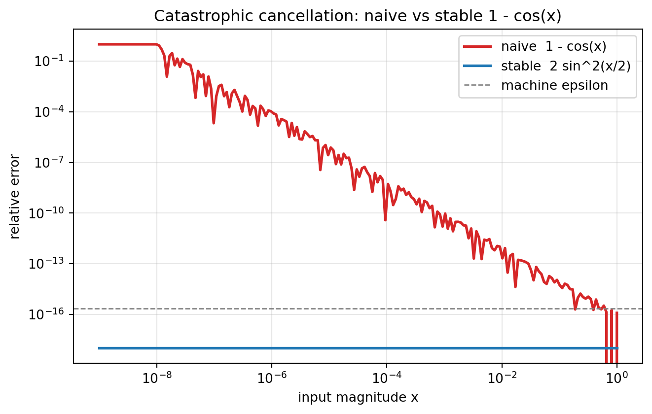
Consider computing \(1 - \cos x\) for small \(x\). Both \(1\) and \(\cos x\) are close to one, so their difference loses most of its significant digits. A numerically superior approach uses the identity \(1 - \cos x = 2 \sin^2(x/2)\), which computes the small quantity directly rather than as a difference of two large ones.

A concrete worked example makes the loss visible. Take \(a = 1.0000000054321\) and \(b = 1.0000000012345\), two numbers that agree in their first nine significant digits. Each is stored in FP64 with a relative error near machine epsilon, roughly \(10^{-16}\). The exact difference is \(a - b = 4.1976 \times 10^{-9}\). The subtraction itself is computed without rounding, since the operands are close enough that their difference is exactly representable. But the absolute error of about \(10^{-16}\) that was already present in each operand now sits on top of a result of magnitude \(10^{-9}\), so the relative error of the difference has been amplified from \(10^{-16}\) to roughly \(10^{-16} / 10^{-9} = 10^{-7}\). Nine digits of accuracy entered the subtraction and only about seven came out. We can frame this with the condition number of subtraction. For \(f(a, b) = a - b\) the relative condition number is \(|a| + |b|\) over \(|a - b|\), which here is about \(2 / (4.2 \times 10^{-9}) \approx 4.8 \times 10^{8}\). A condition number of nearly half a billion means that relative input errors are magnified by that factor, and the worked Python cell below confirms the predicted digit loss numerically.

49.3.2 3.2 The quadratic formula

The standard textbook example is the quadratic formula. When \(b^2 \gg 4ac\), the square root \(\sqrt{b^2 - 4ac}\) is close to \(|b|\), so one of the two roots is computed as the difference of two nearly equal numbers and loses precision. The stable remedy computes the root with the larger magnitude first using the form that adds rather than subtracts,

\[ q = -\tfrac{1}{2}\left(b + \operatorname{sign}(b)\sqrt{b^2 - 4ac}\right), \]

and then recovers the second root from the relationship \(x_1 x_2 = c/a\). The lesson generalizes far beyond quadratics. Whenever an algorithm subtracts two quantities that are nearly equal, look for an algebraic rearrangement that avoids the cancellation. Functions like log1p(x), which computes \(\log(1 + x)\) accurately for small \(x\), and expm1(x), which computes \(e^x - 1\), exist in standard math libraries for exactly this reason.

49.4 4. Conditioning and Stability

49.4.1 4.1 Two distinct ideas

It is essential to separate two concepts that beginners routinely conflate. Conditioning is a property of a mathematical problem. Stability is a property of an algorithm. A problem is ill conditioned if small perturbations in its inputs produce large changes in its exact output, regardless of how you compute that output. An algorithm is unstable if it introduces large errors that the problem itself does not demand.

The condition number quantifies sensitivity. For a differentiable function \(f\), the relative condition number is

\[ \kappa(x) = \left| \frac{x f'(x)}{f(x)} \right|, \]

which measures how a relative change in the input maps to a relative change in the output. For matrix problems, the condition number of \(A\) with respect to inversion is \(\kappa(A) = \|A\| \, \|A^{-1}\|\), equal to the ratio of the largest to the smallest singular value. When \(\kappa(A)\) is large, solving \(Ax = b\) amplifies any error in \(b\), and no algorithm can fully escape that amplification.

49.4.2 4.2 Backward stability

The gold standard for an algorithm is backward stability. An algorithm is backward stable if the answer it computes is the exact answer to a slightly perturbed version of the original problem. Informally, a backward stable algorithm gives you the right answer to nearly the right question. When you combine a backward stable algorithm with a well conditioned problem, you get an accurate result. When the problem is ill conditioned, even a backward stable algorithm produces an output with large error, because the error lives in the problem and not in the method. This is why diagnosing a numerical failure means asking both whether the problem is sensitive and whether the algorithm is sound, since the two failures call for entirely different fixes.

49.5 5. The Log-Sum-Exp Trick

49.5.1 5.1 The overflow problem in probabilistic computation

A great deal of machine learning lives in log space. Likelihoods, partition functions, and attention scores all involve sums of exponentials, and the exponential is the fastest route to overflow that exists in practice. The quantity we frequently need is

\[ \text{LSE}(x_1, \ldots, x_n) = \log \sum_{i=1}^{n} e^{x_i}. \]

If any \(x_i\) is moderately large, say \(100\), then \(e^{x_i}\) overflows FP32 long before the logarithm has a chance to bring it back down. If every \(x_i\) is very negative, each \(e^{x_i}\) underflows to zero, the sum is zero, and the logarithm returns negative infinity. Either way the naive computation fails on inputs that are completely ordinary in a trained network.

49.5.2 5.2 The shift identity

The fix relies on a simple algebraic identity. For any constant \(c\),

\[ \log \sum_{i} e^{x_i} = c + \log \sum_{i} e^{x_i - c}. \]

You can derive this directly. Factor \(e^{c}\) out of every term inside the sum,

\[ \sum_i e^{x_i} = \sum_i e^{c} e^{x_i - c} = e^{c} \sum_i e^{x_i - c}, \]

then take the logarithm of both sides and use \(\log(e^c \cdot S) = c + \log S\),

\[ \log \sum_i e^{x_i} = \log\!\left(e^{c} \sum_i e^{x_i - c}\right) = c + \log \sum_i e^{x_i - c}. \]

The identity holds for any real \(c\), which is the freedom we exploit. The trick is to choose \(c = \max_i x_i\). After the shift, the largest exponent becomes exactly zero, so the largest term in the sum is \(e^0 = 1\) and overflow is impossible. Every other term lies in \((0, 1]\), and any terms that underflow to zero were genuinely negligible relative to the maximum, so the result is unaffected. The stable computation is

c = max(x)
lse = c + log(sum(exp(xi - c) for xi in x))

This pattern, subtract the maximum, exponentiate, sum, take the log, and add the maximum back, is one of the most important numerical idioms in all of machine learning. It appears under different names throughout deep learning libraries, and it is the engine behind the stable softmax.

49.6 6. Stable Softmax and Cross-Entropy

49.6.1 6.1 Softmax

The softmax function turns a vector of real valued scores into a probability distribution,

\[ \text{softmax}(x)_i = \frac{e^{x_i}}{\sum_{j} e^{x_j}}. \]

The naive implementation exponentiates each score directly, which overflows the moment any score is large. The stable version subtracts the maximum score before exponentiating,

\[ \text{softmax}(x)_i = \frac{e^{x_i - c}}{\sum_{j} e^{x_j - c}}, \qquad c = \max_j x_j. \]

This is mathematically identical to the original, since the factor \(e^{-c}\) cancels between numerator and denominator, but now the largest exponent is zero and the computation cannot overflow. Underflow in the smaller terms is benign, because those probabilities round to a tiny value that is genuinely close to zero.

49.6.2 6.2 Why you should fuse softmax with the loss

A subtle but important trap appears when you compute softmax and then feed its output into a cross-entropy loss. The cross-entropy for a true class \(y\) is \(-\log p_y\), where \(p_y\) is the softmax probability of the correct class. If you compute the softmax first and then take its logarithm, you pay twice. The softmax may produce a probability that has underflowed to zero, and then the logarithm of zero is negative infinity, which propagates as NaN once it meets a gradient.

The robust approach computes the log probability directly without ever materializing the bare probability. Using the log-sum-exp result,

\[ \log \text{softmax}(x)_i = x_i - \text{LSE}(x) = (x_i - c) - \log \sum_{j} e^{x_j - c}. \]

The cross-entropy loss then becomes

\[ \mathcal{L} = -\log \text{softmax}(x)_y = \text{LSE}(x) - x_y, \]

which never forms the small probability explicitly and never takes the logarithm of a number that might be zero. This is exactly why mature frameworks provide a single fused operation that takes raw scores, the logits, and the target labels together rather than asking you to chain a softmax into a separate log and a separate negative log likelihood. The fused form is both more accurate and faster, and you should reach for it by default. Passing already normalized probabilities into a loss that expects logits is a common and damaging mistake.

49.6.3 6.3 Gradients in the fused form

There is a further reward for fusing. The gradient of the softmax cross-entropy loss with respect to the logits is

\[ \frac{\partial \mathcal{L}}{\partial x_i} = \text{softmax}(x)_i - \mathbb{1}[i = y], \]

which is the predicted distribution minus the one hot target. This expression is bounded, well behaved, and requires no division by a possibly tiny probability. A naive chain of separate operations would compute a gradient that divides by \(p_y\), reintroducing exactly the instability the fused form was designed to avoid. The clean gradient is one more reason the fused loss is the standard.

49.7 7. Gradient Overflow and Underflow

49.7.1 7.1 Exploding and vanishing magnitudes

During backpropagation, gradients are products of many Jacobian factors chained through the layers of a network. When the factors are consistently larger than one, the product grows exponentially with depth and the gradient overflows to infinity, a phenomenon called exploding gradients. When the factors are consistently smaller than one, the product shrinks exponentially and the gradient underflows toward zero, the vanishing gradient problem. Both are extreme cases of the same multiplicative dynamics, and both are most visible in deep or recurrent architectures where the chain is long.

49.7.2 7.2 Practical defenses

Several techniques keep gradient magnitudes in a workable range. Gradient clipping bounds the global norm of the gradient vector, rescaling it whenever its norm exceeds a threshold \(\tau\),

\[ g \leftarrow g \cdot \min\left(1, \frac{\tau}{\|g\|}\right), \]

which preserves direction while capping magnitude and reliably prevents the occasional exploding step from corrupting the weights. Normalization layers, careful weight initialization that keeps the variance of activations roughly constant across depth, and residual connections that provide a direct gradient path all attack the vanishing side by keeping the per layer Jacobian close to an identity scaling. These are not merely optimization tricks. They are numerical stabilizers that keep the computation inside the representable range of the floating point format.

49.8 8. Mixed-Precision in Deep Learning

49.8.1 8.1 Why low precision at all

Modern accelerators compute far faster in 16 bit formats than in 32 bit, and 16 bit values halve memory traffic and storage. Training large models in pure FP32 leaves most of this throughput unused. Mixed-precision training captures the speed of 16 bit arithmetic while preserving enough 32 bit computation to keep the result correct. The strategy is to store and multiply in low precision where it is safe and to accumulate and update in high precision where it is necessary.

49.8.2 8.2 FP16 versus BF16

Two 16 bit formats dominate. FP16 uses 5 exponent bits and 10 fraction bits, giving good precision but a narrow dynamic range that tops out around \(6.5 \times 10^4\). BF16, the brain floating point format, uses 8 exponent bits and 7 fraction bits, matching the dynamic range of FP32 while sacrificing precision. The trade is direct. FP16 represents nearby values more finely but overflows and underflows easily, while BF16 spans the same enormous range as FP32 and therefore rarely overflows, at the cost of coarser steps between values. Because the failure mode that wrecks training is usually range rather than resolution, BF16 has become the preferred format on hardware that supports it, and it often needs no special scaling at all.

49.8.3 8.3 Loss scaling

FP16 training requires an extra defense because gradients are frequently small enough to underflow the FP16 range and flush to zero, silently halting learning. Loss scaling solves this by multiplying the loss by a large constant \(S\) before backpropagation. By the chain rule every gradient is scaled by the same \(S\), shifting the whole distribution of gradient values up into the representable range. After the backward pass the gradients are divided by \(S\) before the optimizer applies them, so the update is mathematically unchanged.

scaled_loss = loss * S
scaled_loss.backward()
grads = [g / S for g in grads]   # unscale before the optimizer step
optimizer.step()

Dynamic loss scaling automates the choice of \(S\). It raises the scale when training is healthy and, whenever a gradient overflows to infinity, it skips that update and lowers the scale. This adaptive control keeps the gradient distribution near the top of the FP16 range without manual tuning, and it is the default in modern automatic mixed-precision implementations.

49.8.4 8.4 The master weights pattern

The final piece is keeping a high precision copy of the parameters. Weight updates are often tiny relative to the weights themselves, so adding an update to a 16 bit weight can be absorbed entirely, the same vanishing problem from Section 2.2. Mixed-precision training therefore maintains a master copy of the weights in FP32. The forward and backward passes run in 16 bit for speed, but the optimizer applies its update to the FP32 master copy, which is then rounded back to 16 bit for the next iteration. This keeps the slow accumulation of many small updates from being lost to absorption while still reaping the throughput of low precision arithmetic. The recurring theme of the whole chapter is visible here in miniature: compute fast where you can, accumulate carefully where you must, and always keep the critical reductions in the precision the mathematics demands.

49.9 9. Worked Examples in Code

The three hazards above are easiest to believe once you watch them happen. The following cell is executable. It demonstrates catastrophic cancellation against its condition number, the overflow of naive softmax against the stable shifted form, and the error amplification of an ill conditioned linear solve. The random seed is fixed so the output is reproducible.

import numpy as np

rng = np.random.default_rng(0)

# 1. Catastrophic cancellation
a = np.float64(1.0000000054321)
b = np.float64(1.0000000012345)
exact = 4.1976e-9
diff = a - b
rel_err = abs(diff - exact) / exact
cond = (abs(a) + abs(b)) / abs(diff)
print("Catastrophic cancellation")
print(f"  a - b            = {diff:.6e}")
print(f"  relative error   = {rel_err:.2e}")
print(f"  condition number = {cond:.2e}")

# stable 1 - cos x via 2 sin^2(x/2)
x = 1e-8
naive_c = 1.0 - np.cos(x)
stable_c = 2.0 * np.sin(x / 2.0) ** 2
print(f"  1-cos(1e-8) naive  = {naive_c:.3e}")
print(f"  1-cos(1e-8) stable = {stable_c:.3e}")

# 2. Naive vs stable softmax
logits = np.array([1000.0, 1001.0, 1002.0])
with np.errstate(over="ignore", invalid="ignore"):
    naive_sm = np.exp(logits) / np.sum(np.exp(logits))
c = np.max(logits)
stable_sm = np.exp(logits - c) / np.sum(np.exp(logits - c))
print("\nSoftmax overflow")
print(f"  naive  = {naive_sm}")
print(f"  stable = {stable_sm}")

# fused cross-entropy via log-sum-exp
y = 2
lse = c + np.log(np.sum(np.exp(logits - c)))
loss = lse - logits[y]
print(f"  fused cross-entropy loss = {loss:.6f}")

# 3. Conditioning of a linear solve
A = np.array([[1.0, 1.0], [1.0, 1.0 + 1e-10]])
b_vec = np.array([2.0, 2.0])
x_sol = np.linalg.solve(A, b_vec)
x_pert = np.linalg.solve(A, b_vec + np.array([0.0, 1e-8]))
print("\nConditioning")
print(f"  kappa(A)            = {np.linalg.cond(A):.2e}")
print(f"  solution            = {x_sol}")
print(f"  perturbed solution  = {x_pert}")

# Visualize catastrophic cancellation: relative error of naive 1 - cos(x)
# versus the stable form 2 sin^2(x/2) as x shrinks toward zero.
import matplotlib.pyplot as plt

xs = np.logspace(-9, 0, 200)
exact_vals = 2.0 * np.sin(xs / 2.0) ** 2          # accurate reference
naive_vals = 1.0 - np.cos(xs)                      # cancellation prone
stable_vals = 2.0 * np.sin(xs / 2.0) ** 2          # stable rewrite

naive_relerr = np.abs(naive_vals - exact_vals) / exact_vals
stable_relerr = np.abs(stable_vals - exact_vals) / exact_vals
stable_relerr = np.maximum(stable_relerr, 1e-18)   # floor for log axis

fig, ax = plt.subplots(figsize=(7, 4.5))
ax.loglog(xs, naive_relerr, label="naive  1 - cos(x)", color="#d62728", lw=2)
ax.loglog(xs, stable_relerr, label="stable  2 sin^2(x/2)", color="#1f77b4", lw=2)
ax.axhline(np.finfo(np.float64).eps, color="gray", ls="--", lw=1,
           label="machine epsilon")
ax.set_xlabel("input magnitude x")
ax.set_ylabel("relative error")
ax.set_title("Catastrophic cancellation: naive vs stable 1 - cos(x)")
ax.legend()
ax.grid(True, which="both", alpha=0.3)
fig.tight_layout()
plt.show()

Catastrophic cancellation
  a - b            = 4.197600e-09
  relative error   = 1.08e-08
  condition number = 4.76e+08
  1-cos(1e-8) naive  = 0.000e+00
  1-cos(1e-8) stable = 5.000e-17

Softmax overflow
  naive  = [nan nan nan]
  stable = [0.09003057 0.24472847 0.66524096]
  fused cross-entropy loss = 0.407606

Conditioning
  kappa(A)            = 4.00e+10
  solution            = [2. 0.]
  perturbed solution  = [-97.99999112  99.99999112]

The naive softmax returns NaN because \(e^{1002}\) overflows FP64, while the shifted version returns a clean distribution. The linear solve shows a relative input change near \(10^{-9}\) producing a relative output change of order \(10\), exactly the amplification its condition number of \(4 \times 10^{10}\) predicts.

49.10 10. The Stable Softmax Across Languages

The shifted softmax is the same algorithm in any language. The pattern is always subtract the maximum, exponentiate, then normalize. Below the Python version is executable and the others are illustrative.

Python

import numpy as np

def softmax(x):
    x = np.asarray(x, dtype=np.float64)
    z = x - np.max(x)        # shift for stability
    e = np.exp(z)
    return e / np.sum(e)

print(softmax([1000.0, 1001.0, 1002.0]))

[0.09003057 0.24472847 0.66524096]

Julia

function softmax(x::AbstractVector{<:Real})
    c = maximum(x)            # shift for stability
    e = exp.(x .- c)
    return e ./ sum(e)
end

println(softmax([1000.0, 1001.0, 1002.0]))

Rust

fn softmax(x: &[f64]) -> Vec<f64> {
    let c = x.iter().cloned().fold(f64::NEG_INFINITY, f64::max);
    let exps: Vec<f64> = x.iter().map(|&v| (v - c).exp()).collect();
    let sum: f64 = exps.iter().sum();
    exps.iter().map(|&e| e / sum).collect()
}

fn main() {
    let p = softmax(&[1000.0, 1001.0, 1002.0]);
    println!("{:?}", p);
}

49.11 References

1. IEEE. IEEE Standard for Floating-Point Arithmetic (IEEE 754-2019). IEEE, 2019. https://doi.org/10.1109/IEEESTD.2019.8766229
2. Goldberg, D. “What Every Computer Scientist Should Know About Floating-Point Arithmetic.” ACM Computing Surveys, 23(1), 5 to 48, 1991. https://doi.org/10.1145/103162.103163
3. Higham, N. J. Accuracy and Stability of Numerical Algorithms, 2nd ed. SIAM, 2002. https://doi.org/10.1137/1.9780898718027
4. Trefethen, L. N., and Bau, D. Numerical Linear Algebra. SIAM, 1997. https://doi.org/10.1137/1.9780898719574
5. Goodfellow, I., Bengio, Y., and Courville, A. Deep Learning, Chapter 4: Numerical Computation. MIT Press, 2016. https://www.deeplearningbook.org/contents/numerical.html
6. Micikevicius, P., et al. “Mixed Precision Training.” International Conference on Learning Representations (ICLR), 2018. https://doi.org/10.48550/arXiv.1710.03740
7. Kalamkar, D., et al. “A Study of BFLOAT16 for Deep Learning Training.” arXiv preprint, 2019. https://doi.org/10.48550/arXiv.1905.12322
8. Pascanu, R., Mikolov, T., and Bengio, Y. “On the Difficulty of Training Recurrent Neural Networks.” International Conference on Machine Learning (ICML), 28(3), 1310 to 1318, 2013. https://doi.org/10.48550/arXiv.1211.5063
9. Blanchard, P., Higham, D. J., and Higham, N. J. “Accurately Computing the Log-Sum-Exp and Softmax Functions.” IMA Journal of Numerical Analysis, 41(4), 2311 to 2330, 2021. https://doi.org/10.1093/imanum/draa038
10. Kahan, W. “Pracniques: Further Remarks on Reducing Truncation Errors.” Communications of the ACM, 8(1), 40, 1965. https://doi.org/10.1145/363707.363723