111  Gradient Boosting

Gradient boosting is one of the most effective and widely deployed families of supervised learning algorithms for structured, tabular data. It powers winning entries in countless machine learning competitions, drives ranking systems at large search engines, and serves as a default workhorse for credit scoring, fraud detection, and demand forecasting. Its enduring appeal stems from a single elegant idea: a complex predictive function can be built incrementally as a sum of many weak learners, where each new learner is fit to correct the mistakes of the ensemble built so far. This chapter develops that idea rigorously, framing boosting as gradient descent performed in a space of functions rather than a space of parameters. We then turn to the practical machinery that makes the method work in the real world: pseudo-residuals, learning rate and shrinkage, stochastic subsampling, and the several forms of regularization that control overfitting.

111.1 1. From Additive Models to Functional Gradient Descent

111.1.1 1.1 The additive ensemble

Suppose we observe training data \(\{(x_i, y_i)\}_{i=1}^{n}\) with inputs \(x_i \in \mathbb{R}^d\) and targets \(y_i\). We seek a prediction function \(F(x)\) that minimizes the expected loss \(\mathbb{E}[L(y, F(x))]\) for some differentiable loss \(L\). Gradient boosting restricts \(F\) to the class of additive expansions

\[ F_M(x) = \sum_{m=1}^{M} \nu \, h_m(x), \]

where each \(h_m\) is a base learner drawn from some hypothesis class \(\mathcal{H}\) (typically shallow regression trees) and \(\nu\) is a scalar weight. Rather than optimizing all \(M\) terms jointly, which is intractable, the model is built in a greedy stagewise fashion. At stage \(m\) we hold the existing ensemble \(F_{m-1}\) fixed and add one new term:

\[ F_m(x) = F_{m-1}(x) + \nu \, h_m(x). \]

This stagewise structure is the defining characteristic of boosting and the key to its tractability. Each stage is a relatively easy single learner fit; the difficulty of the global problem is amortized across many simple steps.

111.1.2 1.2 Boosting as descent in function space

The central insight, formalized by Friedman in 2001 and developed in parallel by Mason and colleagues, is that stagewise additive modeling is gradient descent carried out in a function space. To see this, regard the empirical risk as a functional of the vector of predictions at the training points. Let \(\mathbf{F} = (F(x_1), \dots, F(x_n))\) and define

\[ J(\mathbf{F}) = \sum_{i=1}^{n} L(y_i, F(x_i)). \]

Ordinary gradient descent on this objective would update each component by stepping in the direction of the negative gradient,

\[ g_i = \left. \frac{\partial L(y_i, F(x_i))}{\partial F(x_i)} \right|_{F = F_{m-1}}, \]

producing the update \(F(x_i) \leftarrow F(x_i) - \nu \, g_i\). The trouble is that this only tells us how to change the predictions at the \(n\) observed points. It gives no recipe for a function defined everywhere on the input space, which is what we need in order to predict on new data.

Gradient boosting resolves this by approximating the negative gradient with a base learner. We fit \(h_m \in \mathcal{H}\) so that its outputs \(h_m(x_i)\) are as close as possible to the negative gradient components \(-g_i\), usually in a least squares sense:

\[ h_m = \arg\min_{h \in \mathcal{H}} \sum_{i=1}^{n} \big( -g_i - h(x_i) \big)^2. \]

The fitted learner \(h_m\) is a smooth, generalizable surrogate for the negative gradient direction. Adding \(\nu \, h_m\) to the ensemble takes a step that decreases the empirical risk while remaining a genuine function over the whole input space. In this view the base learner class \(\mathcal{H}\) plays the role of the set of allowable descent directions, and boosting is steepest descent constrained to that set.

111.2 2. Pseudo-Residuals

111.2.1 2.1 Definition and intuition

The negative gradient components \(-g_i\) are called the pseudo-residuals of the model at stage \(m\). The name is deliberate. For squared error loss \(L(y, F) = \tfrac{1}{2}(y - F)^2\), the gradient is

\[ \frac{\partial L}{\partial F} = -(y - F), \]

so the pseudo-residual is exactly \(-g_i = y_i - F_{m-1}(x_i)\), the ordinary residual. Each tree is therefore fit to the part of the target that the current ensemble has not yet explained. This recovers the intuitive picture of boosting as iterative error correction. For other loss functions the pseudo-residuals are no longer literal residuals, but they retain the same role: they point in the direction that most rapidly reduces the loss at each training point.

111.2.2 2.2 Pseudo-residuals for common losses

The choice of loss determines the form of the pseudo-residuals and thereby the behavior of the algorithm. A few important cases:

For absolute error \(L(y, F) = |y - F|\), the pseudo-residual is the sign of the residual,

\[ -g_i = \operatorname{sign}(y_i - F_{m-1}(x_i)). \]

Because only the sign enters, large errors do not dominate the fit, which makes the method robust to outliers in the response.

For the Huber loss, which is quadratic for small residuals and linear beyond a threshold \(\delta\), the pseudo-residual interpolates between these two regimes, combining the efficiency of squared error near the optimum with the robustness of absolute error in the tails.

For binary classification with the logistic (binomial deviance) loss, working with \(y_i \in \{0, 1\}\) and modeling the log-odds \(F(x)\), the loss is

\[ L(y, F) = -\big[\, y \log p + (1 - y) \log(1 - p) \,\big], \qquad p = \frac{1}{1 + e^{-F}}. \]

Differentiating gives the pseudo-residual

\[ -g_i = y_i - p_i = y_i - \frac{1}{1 + e^{-F_{m-1}(x_i)}}. \]

This is the difference between the observed label and the predicted probability, a clean and interpretable signal. For multiclass problems the softmax cross entropy generalizes this, yielding one set of pseudo-residuals per class.

111.2.3 2.3 Line search and leaf values

Fitting a tree to pseudo-residuals tells us the partition of the input space, but the optimal output value within each leaf still depends on the loss. After the tree structure is fixed, gradient boosting performs a separate one dimensional optimization for each terminal region \(R_{jm}\):

\[ \gamma_{jm} = \arg\min_{\gamma} \sum_{x_i \in R_{jm}} L\big(y_i, F_{m-1}(x_i) + \gamma\big). \]

For squared error this line search returns the mean of the residuals in the leaf, but for other losses it gives a different, loss aware value. The tree then contributes \(\sum_j \gamma_{jm} \mathbf{1}(x \in R_{jm})\). This two phase procedure, fit structure to the gradient then choose leaf values by line search, is what distinguishes gradient boosting from naively regressing on residuals.

111.3 3. The Generic Algorithm

We can now assemble the components into the canonical gradient boosting procedure of Friedman.

The following implements the procedure from scratch for squared error loss, where the pseudo-residual is the ordinary residual and the line search reduces to fitting each tree on that residual. We boost on a noisy one dimensional function and report how well the additive ensemble recovers the underlying signal.

import numpy as np
from sklearn.tree import DecisionTreeRegressor

rng = np.random.default_rng(0)
X = np.linspace(-3, 3, 200).reshape(-1, 1)
y_true = np.sin(X).ravel() + 0.3 * X.ravel()
y = y_true + rng.normal(0, 0.25, size=X.shape[0])

nu = 0.1
M = 200
init = y.mean()                              # F_0 = mean (squared-error optimum)
F = np.full(X.shape[0], init)
trees = []
for m in range(M):
    residual = y - F                         # pseudo-residual for squared error
    tree = DecisionTreeRegressor(max_depth=2)
    tree.fit(X, residual)
    F = F + nu * tree.predict(X)             # update with shrinkage nu
    trees.append(tree)

final = F
print("train MSE after", M, "trees:", round(float(np.mean((y - final) ** 2)), 4))
print("MSE vs true signal:", round(float(np.mean((y_true - final) ** 2)), 4))

train MSE after 200 trees: 0.023
MSE vs true signal: 0.0177

The ensemble fits the noisy targets while tracking the clean signal even more closely, since the slow shrinkage averages over the noise rather than memorizing it.

The initial model \(F_0\) is a constant that minimizes the loss over the training set: the mean for squared error, the median for absolute error, the log-odds of the base rate for logistic loss. Every subsequent stage refines this constant by one tree. The hyperparameters that govern the procedure (the learning rate \(\nu\), the number of trees \(M\), the tree depth, the subsampling rates, and the regularization penalties) are the subject of the remaining sections.

111.4 4. Learning Rate and Shrinkage

111.4.1 4.1 Shrinkage as regularization

The learning rate \(\nu\), also called the shrinkage parameter, scales the contribution of each tree before it is added to the ensemble. Setting \(\nu = 1\) takes the full line search step; setting \(\nu < 1\) deliberately takes a smaller step, so that each tree corrects only a fraction of the residual it was fit to. Friedman observed empirically that small values of \(\nu\), typically in the range \(0.01\) to \(0.1\), substantially improve generalization. The mechanism is a form of regularization. By forcing the ensemble to make slow, incremental progress, shrinkage prevents any single tree from over committing to idiosyncratic structure in the training data, and it spreads the modeling effort across many trees so that the resulting function is smoother.

111.4.2 4.2 The tradeoff with the number of trees

Shrinkage and the number of trees \(M\) are coupled. A smaller learning rate requires more trees to reach a given training loss, since each step covers less ground. As a rough rule, halving \(\nu\) roughly doubles the \(M\) needed for comparable fit. The two cannot be tuned independently; they trade off along a curve. The practical guidance that has emerged from years of experience is to fix \(\nu\) at a small value the computational budget allows and then choose \(M\) as large as that budget permits, using early stopping on a validation set to halt training once the held out loss stops improving.

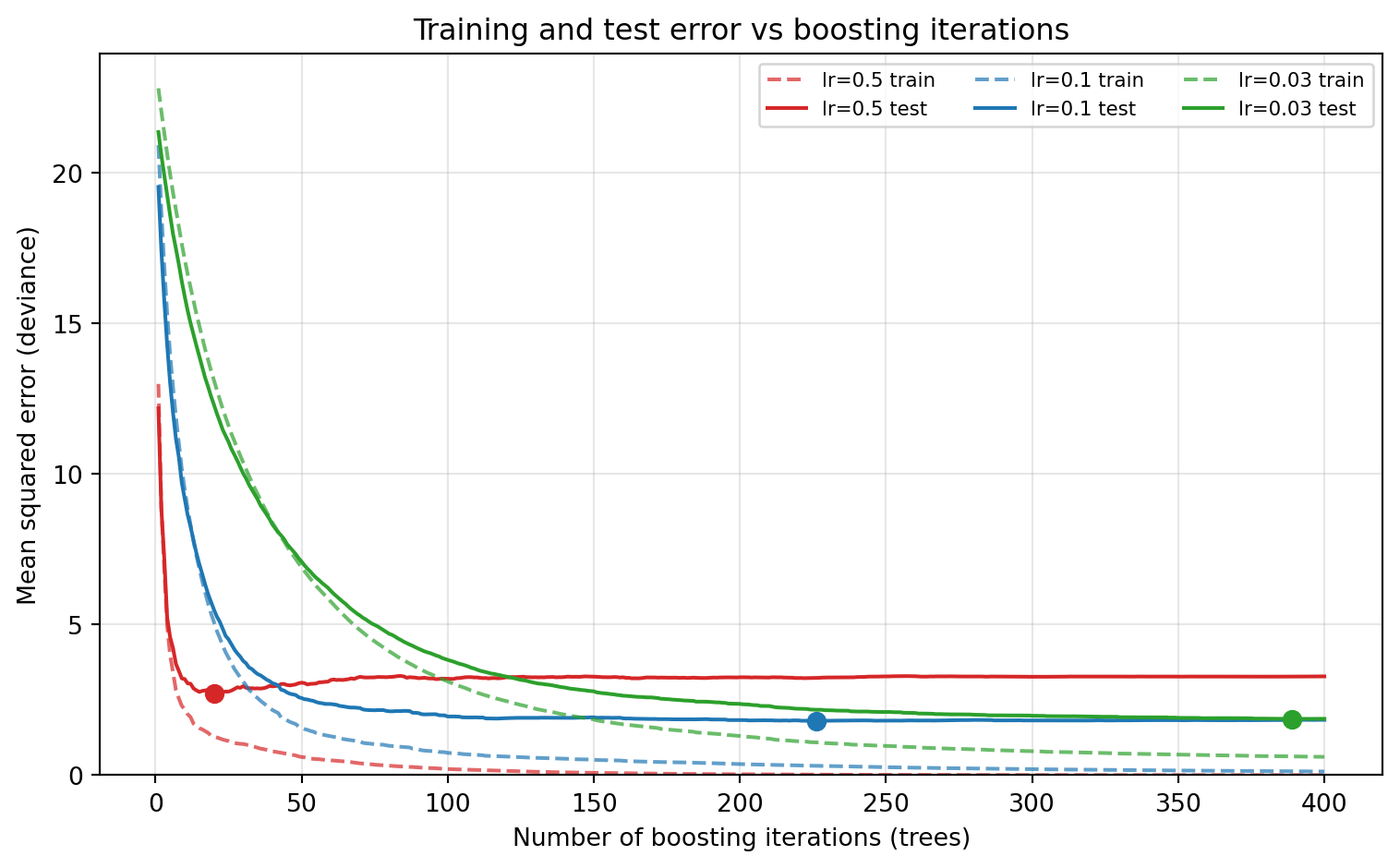
We can watch this tradeoff directly. Using staged_predict to evaluate the test error after every added tree, the cell below sweeps three learning rates and reports the best test error and the number of trees at which it occurs. Smaller rates need more trees but reach a lower, broader minimum.

import numpy as np
import matplotlib.pyplot as plt
from sklearn.datasets import make_friedman1
from sklearn.model_selection import train_test_split
from sklearn.ensemble import GradientBoostingRegressor
from sklearn.metrics import mean_squared_error

np.random.seed(42)
Xf, yf = make_friedman1(n_samples=1200, noise=1.0, random_state=42)
Xtr, Xte, ytr, yte = train_test_split(Xf, yf, test_size=0.3, random_state=42)

n_estimators = 400
iters = np.arange(1, n_estimators + 1)
curves = {}
for lr in (0.5, 0.1, 0.03):
    gbr = GradientBoostingRegressor(
        n_estimators=n_estimators, learning_rate=lr, max_depth=3,
        subsample=0.7, random_state=0)
    gbr.fit(Xtr, ytr)
    train_err = [mean_squared_error(ytr, p) for p in gbr.staged_predict(Xtr)]
    test_err = [mean_squared_error(yte, p) for p in gbr.staged_predict(Xte)]
    curves[lr] = (np.array(train_err), np.array(test_err))
    best_iter = int(np.argmin(test_err)) + 1
    print(f"lr={lr}: best test MSE={min(test_err):.3f} at {best_iter} trees")

fig, ax = plt.subplots(figsize=(8, 5))
colors = {0.5: "tab:red", 0.1: "tab:blue", 0.03: "tab:green"}
for lr, (train_err, test_err) in curves.items():
    c = colors[lr]
    ax.plot(iters, train_err, color=c, linestyle="--", alpha=0.7,
            label=f"lr={lr} train")
    ax.plot(iters, test_err, color=c, linestyle="-",
            label=f"lr={lr} test")
    best = int(np.argmin(test_err))
    ax.plot(best + 1, test_err[best], "o", color=c, markersize=7)

ax.set_xlabel("Number of boosting iterations (trees)")
ax.set_ylabel("Mean squared error (deviance)")
ax.set_title("Training and test error vs boosting iterations")
ax.set_ylim(0, None)
ax.legend(ncol=3, fontsize=8)
ax.grid(True, alpha=0.3)
fig.tight_layout()
plt.show()

lr=0.5: best test MSE=2.725 at 20 trees
lr=0.1: best test MSE=1.802 at 226 trees
lr=0.03: best test MSE=1.865 at 389 trees

The large rate overshoots and bottoms out early at a worse error; the small rates climb more slowly to a better minimum. The combination of small \(\nu\) and large \(M\) with early stopping is close to a free lunch for accuracy, paid for only in training time. This is why nearly every modern gradient boosting library defaults to a modest learning rate and exposes early stopping as a first class feature.

111.4.3 4.3 A connection to learning rates in parametric optimization

The shrinkage parameter plays exactly the role of the step size in classical gradient descent. In parameter space, too large a step overshoots and destabilizes; too small a step converges slowly but reliably and tends to find flatter, better generalizing optima. The same intuition transfers to function space. Shrinkage is the functional analogue of a small, carefully chosen learning rate, and the well known interaction between step size and number of iterations carries over directly to the interaction between \(\nu\) and \(M\).

111.5 5. Stochastic Gradient Boosting and Subsampling

111.5.1 5.1 Row subsampling

In 2002 Friedman introduced stochastic gradient boosting, a modification that draws a random subsample of the training rows, without replacement, at each iteration and fits the tree only to that subsample. The subsampling fraction, often denoted \(\eta\) or subsample, typically lies between \(0.5\) and \(0.8\). This injection of randomness has two beneficial effects. First, it reduces the correlation between successive trees, much as bagging decorrelates the trees in a random forest, which lowers the variance of the ensemble and improves accuracy. Second, fitting on a fraction of the data reduces the per iteration cost, so training is faster.

The pseudo-residuals are still computed for the rows in the current subsample using the full current model, and the line search for leaf values is restricted to those rows. The next iteration draws a fresh subsample. Empirically, a subsample fraction below one almost always helps when the dataset is large enough to tolerate the reduced sample per tree, and it can be viewed as a regularizer in its own right.

111.5.2 5.2 Column subsampling

Borrowing another idea from random forests, modern implementations also support column subsampling: at each tree, or at each split, only a random subset of the features is considered as candidate split variables. Controlled by parameters such as colsample_bytree and colsample_bylevel, this further decorrelates trees and provides robustness when many features are noisy or redundant. Column subsampling is especially valuable in high dimensional settings where a few dominant features would otherwise be chosen repeatedly, starving the ensemble of diversity.

111.5.3 5.3 Why injected randomness helps

The generalization error of an ensemble decomposes loosely into bias, variance, and a term governed by the correlation among its members. Boosting is primarily a bias reduction method: each stage chips away at the residual error. Subsampling adds a variance reduction mechanism on top, by ensuring that the trees are not all responding to the same fine grained patterns in the same data. The result is an ensemble that retains the low bias of boosting while enjoying some of the variance reduction of bagging. The optimal subsampling rate is data dependent and is best treated as a hyperparameter to tune.

111.6 6. Regularization

Beyond shrinkage and subsampling, several explicit regularization controls keep gradient boosting from overfitting. They fall into two groups: constraints on the structure of individual trees, and penalties added to the objective.

111.6.1 6.1 Tree complexity constraints

The most important structural control is the depth or, equivalently, the number of leaves of each tree. Shallow trees, with depth between three and eight or a few dozen leaves, capture only low order feature interactions and act as genuinely weak learners. Deep trees model high order interactions and can overfit quickly, which is why depth is rarely set large in boosting. Additional structural constraints include a minimum number of samples required to split a node, a minimum number of samples (or minimum sum of instance weights) per leaf, and a minimum loss reduction required to make a split. The last of these, often called gamma or min_split_loss, prunes splits whose gain does not exceed a threshold, directly limiting model complexity.

111.6.2 6.2 Penalized objectives and the second order view

Modern libraries such as XGBoost optimize a regularized objective that adds an explicit complexity penalty to each tree. Writing the tree as \(h(x) = \sum_{j=1}^{T} w_j \mathbf{1}(x \in R_j)\) with \(T\) leaves and leaf weights \(w_j\), the penalty takes the form

\[ \Omega(h) = \gamma\, T + \frac{1}{2} \lambda \sum_{j=1}^{T} w_j^2 + \alpha \sum_{j=1}^{T} |w_j|, \]

where \(\gamma\) penalizes the number of leaves, \(\lambda\) applies an \(L_2\) penalty to the leaf weights, and \(\alpha\) applies an \(L_1\) penalty. These shrink the leaf values toward zero and discourage overly complex trees.

To compute the optimal leaf weights under this objective, XGBoost uses a second order Taylor expansion of the loss around the current predictions. Let \(g_i\) and \(h_i\) denote the first and second derivatives of the loss with respect to the prediction at point \(i\). The approximate objective for adding a tree is

\[ \tilde{J} = \sum_{i=1}^{n} \Big[ g_i\, h(x_i) + \tfrac{1}{2} h_i\, h(x_i)^2 \Big] + \Omega(h). \]

For a fixed tree structure, the optimal weight in leaf \(j\) (with \(L_1\) set aside for clarity) is

\[ w_j^\star = -\frac{\sum_{i \in R_j} g_i}{\sum_{i \in R_j} h_i + \lambda}, \]

and the corresponding reduction in the objective gives a principled split gain that is used to grow the tree greedily. The appearance of \(\lambda\) in the denominator shows directly how \(L_2\) regularization shrinks leaf values: larger \(\lambda\) pulls every weight toward zero. This second order formulation, due to Chen and Guestrin, is one reason XGBoost converges in fewer iterations than first order gradient boosting and why its regularization is so effective.

111.6.3 6.3 Early stopping

Perhaps the simplest and most powerful regularizer is early stopping. Because boosting adds trees one at a time, the validation loss can be monitored after each tree, and training halts when it fails to improve for a fixed number of rounds. Early stopping selects the effective number of trees automatically, adapting \(M\) to the data without a separate search. It interacts cleanly with a small learning rate: the slow, incremental progress of shrinkage means the validation curve has a broad, well defined minimum that is easy to detect.

111.6.4 6.4 Other regularizers

Several implementations offer additional mechanisms. DART, available in XGBoost and LightGBM, applies dropout to trees during boosting, randomly muting a subset of existing trees when computing each new one, which prevents later trees from over specializing to the errors of the first few. Monotonic constraints force the predicted function to be nondecreasing or nonincreasing in chosen features, encoding domain knowledge and reducing variance. Feature interaction constraints restrict which features may appear together in a tree, limiting model complexity in a structured way. Each of these trades a small amount of flexibility for improved generalization or interpretability.

111.7 7. Practical Synthesis

The hyperparameters of gradient boosting are not independent knobs but an interacting system. A workable strategy that reflects common practice is the following. Fix a small learning rate, around \(0.03\) to \(0.1\). Set a large maximum number of trees and rely on early stopping with a validation set to choose the actual count. Use moderate tree depth, commonly between four and eight, as the primary lever on the bias variance tradeoff. Apply row subsampling near \(0.7\) and column subsampling near \(0.7\) to decorrelate trees and speed training. Finally, tune the explicit penalties (\(\lambda\), \(\gamma\), and minimum child weight) to taste, increasing them if the validation loss diverges from the training loss.

The cell below puts this discipline into practice with scikit-learn’s gradient booster. We set a small learning rate, a generous tree cap, row and column subsampling near \(0.7\), and let validation based early stopping choose the effective number of trees automatically.

import numpy as np
from sklearn.datasets import make_friedman1
from sklearn.model_selection import train_test_split
from sklearn.ensemble import GradientBoostingRegressor

Xf, yf = make_friedman1(n_samples=1500, noise=1.0, random_state=7)
Xtr, Xte, ytr, yte = train_test_split(Xf, yf, test_size=0.3, random_state=7)

gbr = GradientBoostingRegressor(
    n_estimators=5000, learning_rate=0.05, max_depth=6,
    subsample=0.7, max_features=0.7,
    validation_fraction=0.2, n_iter_no_change=50, random_state=1)
gbr.fit(Xtr, ytr)
print("early stopping selected n_trees:", gbr.n_estimators_)
print("test R^2:", round(gbr.score(Xte, yte), 3))

early stopping selected n_trees: 449
test R^2: 0.894

Despite a cap of 5000 trees, early stopping halts after a few hundred, illustrating how it adapts \(M\) to the data without a separate search. These defaults are a starting point, not an answer. The decisive practical discipline is honest validation: a held out set or cross validation that drives early stopping and guides hyperparameter search. With that discipline in place, gradient boosting remains, after two decades, one of the most reliable tools for learning from tabular data.

111.8 8. Summary

Gradient boosting builds a predictive function as a sum of weak learners, adding one at a time. The unifying theory casts this as gradient descent in function space: each stage fits a base learner to the negative gradient of the loss, the pseudo-residuals, and adds a shrunken multiple of it to the ensemble. The form of the pseudo-residuals follows from the chosen loss, allowing the same algorithm to handle regression, classification, ranking, and robust objectives. Learning rate and shrinkage regularize the procedure by slowing its progress, trading off against the number of trees. Stochastic subsampling of rows and columns decorrelates the trees and reduces variance. Explicit penalties on tree complexity, second order optimization of regularized objectives, and early stopping complete the toolkit. Understanding how these pieces fit together, both as theory and as practice, is what lets a practitioner wield gradient boosting effectively rather than merely tune it blindly.

111.9 References

1. Friedman, J. H. (2001). Greedy Function Approximation: A Gradient Boosting Machine. Annals of Statistics, 29(5), 1189 to 1232. https://projecteuclid.org/euclid.aos/1013203451
2. Friedman, J. H. (2002). Stochastic Gradient Boosting. Computational Statistics and Data Analysis, 38(4), 367 to 378. https://www.sciencedirect.com/science/article/pii/S0167947301000652
3. Mason, L., Baxter, J., Bartlett, P., and Frean, M. (2000). Boosting Algorithms as Gradient Descent. Advances in Neural Information Processing Systems 12. https://papers.nips.cc/paper/1999/hash/96a93ba89a5b5c6c226e49b88973f46e-Abstract.html
4. Chen, T., and Guestrin, C. (2016). XGBoost: A Scalable Tree Boosting System. Proceedings of KDD 2016. https://dl.acm.org/doi/10.1145/2939672.2939785
5. Ke, G., Meng, Q., Finley, T., et al. (2017). LightGBM: A Highly Efficient Gradient Boosting Decision Tree. Advances in Neural Information Processing Systems 30. https://papers.nips.cc/paper/2017/hash/6449f44a102fde848669bdd9eb6b76fa-Abstract.html
6. Prokhorenkova, L., Gusev, G., Vorobev, A., Dorogush, A. V., and Gulin, A. (2018). CatBoost: Unbiased Boosting with Categorical Features. Advances in Neural Information Processing Systems 31. https://papers.nips.cc/paper/2018/hash/14491b756b3a51daac41c24863285549-Abstract.html
7. Hastie, T., Tibshirani, R., and Friedman, J. (2009). The Elements of Statistical Learning, 2nd ed., Chapter 10. Springer. https://hastie.su.domains/ElemStatLearn/
8. Rashmi, K. V., and Gilad-Bachrach, R. (2015). DART: Dropouts meet Multiple Additive Regression Trees. Proceedings of AISTATS 2015. https://proceedings.mlr.press/v38/korlakaivinayak15.html