Most interesting questions in machine learning involve more than one random variable at a time. A classifier reasons about a label given an image, a language model predicts a token given a context, and a recommender system models the relationship between users and items. The mathematical machinery that lets us describe how several random variables behave together, and how knowledge of some informs our beliefs about others, is the theory of joint, marginal, and conditional distributions. This chapter develops that machinery in depth, builds up to the chain rule of probability, and then studies the second-order structure captured by covariance and correlation. We close with a detailed treatment of the multivariate Gaussian, the single most important distribution in applied statistics and machine learning.
34.1 1. Joint Distributions
34.1.1 1.1 Defining the Joint Distribution
Consider two random variables \(X\) and \(Y\) defined on the same probability space. The joint distribution describes the probability of events involving both variables simultaneously. In the discrete case, the joint probability mass function (PMF) is
\[
p_{X,Y}(x, y) = P(X = x, Y = y),
\]
where the comma denotes logical conjunction, so we are asking for the probability that \(X = x\) and \(Y = y\) both hold. A valid joint PMF satisfies \(p_{X,Y}(x,y) \ge 0\) for all pairs and sums to one,
\[
\sum_{x} \sum_{y} p_{X,Y}(x, y) = 1.
\]
In the continuous case, the joint probability density function (PDF) \(f_{X,Y}(x,y)\) plays the analogous role, with probabilities recovered by integration over regions:
and the normalization condition becomes a double integral over the whole plane equal to one. The density itself is not a probability; it is a probability per unit area, and it may exceed one as long as the integral is well behaved.
34.1.2 1.2 Why Joint Structure Matters
The joint distribution carries strictly more information than the two variables considered separately. Knowing how often it rains and knowing how often the ground is wet does not tell you whether those two facts move together, but the joint distribution does. In machine learning we frequently posit a joint distribution \(p(x, y)\) over inputs \(x\) and labels \(y\), and the entire supervised learning enterprise can be framed as trying to learn useful properties of that joint object from a finite sample. Generative models such as variational autoencoders and diffusion models go further and attempt to model the full joint density of high-dimensional data directly.
For a vector of \(d\) random variables collected into \(\mathbf{X} = (X_1, \ldots, X_d)\), the joint distribution lives in a \(d\)-dimensional space. The number of parameters needed to specify an arbitrary joint distribution grows exponentially with \(d\), a phenomenon known as the curse of dimensionality. Much of probabilistic modeling consists of imposing structure, such as independence or conditional independence, to make the joint tractable.
34.2 2. Marginalization
34.2.1 2.1 From Joint to Marginal
Given a joint distribution, we often want the distribution of a single variable, ignoring the others. This is the marginal distribution, and the operation that produces it is marginalization. For discrete variables we sum out the variable we wish to discard:
The name comes from a historical practice of writing the row sums and column sums of a tabulated joint distribution in the margins of the table. Marginalization is the probabilistic analogue of projection. We collapse a higher-dimensional object onto a lower-dimensional one by integrating away the directions we do not care about.
34.2.2 2.2 Marginalization in Practice
Marginalization is everywhere in machine learning, and it is frequently the hard part. The evidence in Bayesian inference,
is a marginal obtained by integrating the joint over all parameter values. When we have latent variables \(z\), the likelihood of an observation requires marginalizing them out,
and this integral is intractable for most interesting models. Techniques such as variational inference and Monte Carlo sampling exist precisely because exact marginalization is so often impossible. A key conceptual point is that marginalization respects nothing about the structure of the discarded variable; it simply averages over all of its possible values, weighted by their probability.
34.3 3. Conditional Distributions
34.3.1 3.1 The Definition of Conditioning
Conditioning answers the question: given that I have observed one variable take a particular value, what is the distribution of another? The conditional PMF or PDF is defined as the ratio of the joint to the marginal,
defined wherever the marginal in the denominator is nonzero. Dividing by the marginal renormalizes the slice of the joint at \(X = x\) so that it integrates to one as a proper distribution over \(y\). Geometrically, fixing \(X = x\) selects a one-dimensional slice through the joint density, and the division rescales that slice so that it becomes a valid distribution in its own right.
Rearranging the definition gives the product rule, the foundation for nearly everything that follows:
34.3.2 3.2 Independence and Conditional Independence
Two variables are independent when conditioning on one does not change the distribution of the other, which is equivalent to the joint factoring as the product of marginals,
\[
p_{X,Y}(x, y) = p_X(x)\, p_Y(y) \quad \text{for all } x, y.
\]
A weaker and far more useful notion is conditional independence. We say \(X\) and \(Y\) are conditionally independent given \(Z\), written \(X \perp Y \mid Z\), when
Conditional independence is the cornerstone of probabilistic graphical models. The naive Bayes classifier assumes that features are conditionally independent given the class label, which collapses an intractable joint over features into a simple product. Bayesian networks encode a web of conditional independence assumptions as a directed graph, and those assumptions are exactly what make inference and learning feasible.
34.3.3 3.3 Bayes’ Theorem
Equating the two factorizations of the joint and solving for one conditional yields Bayes’ theorem,
where the denominator is the marginal \(p_Y(y) = \sum_x p_{Y \mid X}(y \mid x)\, p_X(x)\) obtained by marginalization. This deceptively simple identity is the engine of Bayesian machine learning. It tells us how to invert a conditional, turning a model of how data arise given parameters into a posterior belief about parameters given data. The prior \(p_X(x)\), the likelihood \(p_{Y \mid X}(y \mid x)\), and the evidence \(p_Y(y)\) each play a distinct role, and the difficulty of computing the evidence is again a marginalization problem.
34.4 4. The Chain Rule of Probability
34.4.1 4.1 Factorizing a Joint Distribution
The product rule for two variables generalizes to any number of variables. Applying it repeatedly, any joint distribution over \(X_1, \ldots, X_n\) factorizes as a product of conditionals:
This is the chain rule of probability. It holds for any ordering of the variables and requires no assumptions whatsoever; it is a pure consequence of the definition of conditional probability. Different orderings give different but equally valid factorizations, and choosing a convenient ordering is often where modeling insight enters.
34.4.2 4.2 The Chain Rule in Modern Machine Learning
The chain rule underwrites autoregressive modeling, which is the paradigm behind large language models. A language model treats a sentence as a sequence of tokens and factorizes the joint probability of the sequence left to right,
so that generating text reduces to repeatedly sampling the next token from a learned conditional. Each conditional \(p(w_t \mid w_{<t})\) is computed by a neural network, and training maximizes the log probability the chain rule assigns to observed sequences. The same logic drives autoregressive image models such as PixelRNN and the autoregressive components of many other generative architectures. When conditional independence assumptions are layered on top of the chain rule, the long conditioning contexts shrink, and we recover the compact factorizations of graphical models. The chain rule, then, is the bridge between raw probability theory and the structured probabilistic models that dominate the field.
34.5 5. Covariance and Correlation
34.5.1 5.1 Covariance
While the full joint distribution captures all dependence, we often summarize the linear part of that dependence with a single number. The covariance of two random variables measures how they vary together,
where \(\mu_X = \mathbb{E}[X]\) and \(\mu_Y = \mathbb{E}[Y]\). A positive covariance means the variables tend to lie on the same side of their means together, a negative covariance means they tend to lie on opposite sides, and a covariance of zero means there is no linear association. The covariance of a variable with itself is its variance, \(\operatorname{Cov}(X, X) = \operatorname{Var}(X)\).
A crucial subtlety is that independence implies zero covariance, but zero covariance does not imply independence. Two variables can be strongly dependent through a nonlinear relationship while having exactly zero covariance. If \(X\) is symmetric about zero and \(Y = X^2\), then \(X\) and \(Y\) are functionally dependent, yet their covariance vanishes. Covariance sees only linear structure.
The covariance is bilinear in its arguments, a property worth deriving once because it is used constantly. For constants \(a\), \(b\), \(c\), \(d\) and random variables \(X\), \(Y\), \(Z\),
To see this, note that adding constants does not change the deviations from the mean, since \(\mathbb{E}[aX + b] = a\,\mathbb{E}[X] + b\), so \((aX + b) - \mathbb{E}[aX + b] = a(X - \mu_X)\). Substituting into the definition,
A second key property is additivity, \(\operatorname{Cov}(X + Y, Z) = \operatorname{Cov}(X, Z) + \operatorname{Cov}(Y, Z)\), which follows from the linearity of expectation applied to the deviation products. Combining bilinearity with the identity \(\operatorname{Cov}(X, X) = \operatorname{Var}(X)\) gives the variance of a sum,
which reduces to the familiar additivity of variances exactly when \(X\) and \(Y\) are uncorrelated.
34.5.2 5.2 Correlation
Covariance has the awkward property of carrying the product of the units of \(X\) and \(Y\), which makes its magnitude hard to interpret. The Pearson correlation coefficient fixes this by normalizing,
where \(\sigma_X\) and \(\sigma_Y\) are the standard deviations. The bound \(\rho_{X,Y} \in [-1, 1]\) is a direct consequence of the Cauchy-Schwarz inequality, which we can derive cleanly. Center the variables as \(U = X - \mu_X\) and \(V = Y - \mu_Y\), and consider the nonnegative quantity \(\mathbb{E}\big[(tU + V)^2\big] \ge 0\) for every real \(t\). Expanding,
since \(\mathbb{E}[UV] = \operatorname{Cov}(X, Y)\), \(\mathbb{E}[U^2] = \operatorname{Var}(X)\), and \(\mathbb{E}[V^2] = \operatorname{Var}(Y)\). Dividing both sides by \(\sigma_X^2 \sigma_Y^2\) yields \(\rho_{X,Y}^2 \le 1\). Equality holds exactly when \(tU + V = 0\) almost surely for some \(t\), that is, when \(Y\) is an exact linear function of \(X\). A value of \(+1\) indicates a perfect increasing linear relationship, \(-1\) a perfect decreasing one, and \(0\) the absence of linear association. Correlation is dimensionless and invariant to separate positive linear rescalings of each variable, which is why it is the standard tool for reporting the strength of an association. In machine learning, feature correlation analysis guides feature selection, flags redundant predictors, and warns of multicollinearity that can destabilize linear models.
34.6 6. The Covariance Matrix
34.6.1 6.1 Definition and Structure
When we move from two variables to a random vector \(\mathbf{X} = (X_1, \ldots, X_d)^\top\), the pairwise covariances assemble into a matrix. The covariance matrix is
where \(\boldsymbol{\mu} = \mathbb{E}[\mathbf{X}]\) is the mean vector. The entry in row \(i\) and column \(j\) is \(\Sigma_{ij} = \operatorname{Cov}(X_i, X_j)\), so the diagonal holds the variances of the individual components and the off-diagonal entries hold the pairwise covariances. Because \(\operatorname{Cov}(X_i, X_j) = \operatorname{Cov}(X_j, X_i)\), the covariance matrix is symmetric.
34.6.2 6.2 Positive Semidefiniteness
Beyond symmetry, every valid covariance matrix is positive semidefinite, meaning that for any constant vector \(\mathbf{a} \in \mathbb{R}^d\),
The identity follows because \(\mathbf{a}^\top \boldsymbol{\Sigma} \mathbf{a}\) is exactly the variance of the scalar projection \(\mathbf{a}^\top \mathbf{X}\), and a variance can never be negative. Positive semidefiniteness guarantees that all eigenvalues of \(\boldsymbol{\Sigma}\) are nonnegative, which in turn underpins the spectral decomposition used throughout dimensionality reduction.
34.6.3 6.3 The Covariance Matrix and Principal Component Analysis
Principal component analysis (PCA) is the canonical application of the covariance matrix in machine learning. PCA performs an eigendecomposition of \(\boldsymbol{\Sigma}\),
where the columns of \(\mathbf{U}\) are orthonormal eigenvectors and \(\boldsymbol{\Lambda}\) is the diagonal matrix of eigenvalues. The eigenvectors point along the directions of greatest variance in the data, and the corresponding eigenvalues quantify how much variance lies along each direction. Projecting data onto the top few eigenvectors retains most of the variance while discarding noisy or redundant directions, giving a compact representation. The covariance matrix also defines the Mahalanobis distance, \(\sqrt{(\mathbf{x} - \boldsymbol{\mu})^\top \boldsymbol{\Sigma}^{-1} (\mathbf{x} - \boldsymbol{\mu})}\), which measures distance in units that account for the spread and correlation of the data, and which appears as the exponent of the multivariate Gaussian.
34.7 7. The Multivariate Gaussian in Depth
34.7.1 7.1 The Density
The multivariate Gaussian, or multivariate normal, distribution generalizes the familiar bell curve to \(d\) dimensions. A random vector \(\mathbf{X} \in \mathbb{R}^d\) is multivariate Gaussian with mean \(\boldsymbol{\mu}\) and covariance \(\boldsymbol{\Sigma}\), written \(\mathbf{X} \sim \mathcal{N}(\boldsymbol{\mu}, \boldsymbol{\Sigma})\), when its density is
where \(|\boldsymbol{\Sigma}|\) denotes the determinant. The quadratic form in the exponent is the squared Mahalanobis distance, so surfaces of constant density are ellipsoids centered at \(\boldsymbol{\mu}\). The eigenvectors of \(\boldsymbol{\Sigma}\) give the orientation of those ellipsoids, and the square roots of the eigenvalues give their semi-axis lengths. The normalizing constant out front ensures the density integrates to one, with the determinant measuring the volume of the ellipsoid of concentration.
34.7.2 7.2 Marginals and Conditionals
The multivariate Gaussian is special because it is closed under both marginalization and conditioning, and the resulting distributions are again Gaussian with parameters given in closed form. Partition the vector as \(\mathbf{X} = (\mathbf{X}_a, \mathbf{X}_b)\) with the mean and covariance blocked conformably,
The marginal of any sub-vector is read off directly: \(\mathbf{X}_a \sim \mathcal{N}(\boldsymbol{\mu}_a, \boldsymbol{\Sigma}_{aa})\). We simply keep the relevant blocks and discard the rest. The conditional is also Gaussian, with mean and covariance
These formulas repay close study. The conditional mean is a linear function of the observed value \(\mathbf{x}_b\), which is why linear regression with Gaussian assumptions produces linear predictors. The conditional covariance does not depend on \(\mathbf{x}_b\) at all, and it is never larger than the unconditional covariance, capturing the intuition that observing \(\mathbf{x}_b\) can only reduce or maintain our uncertainty about \(\mathbf{x}_a\). The term \(\boldsymbol{\Sigma}_{ab}\boldsymbol{\Sigma}_{bb}^{-1}\boldsymbol{\Sigma}_{ba}\) is the variance explained by the observation.
34.7.2.1 Deriving the conditional
The conditioning formulas are not magic; they fall out of completing the square in the exponent. The cleanest derivation uses the block inverse of \(\boldsymbol{\Sigma}\), written in terms of the Schur complement \(\mathbf{S} = \boldsymbol{\Sigma}_{aa} - \boldsymbol{\Sigma}_{ab} \boldsymbol{\Sigma}_{bb}^{-1} \boldsymbol{\Sigma}_{ba}\). The inverse covariance, or precision matrix, has the block form
The conditional density \(f(\mathbf{x}_a \mid \mathbf{x}_b) \propto f(\mathbf{x}_a, \mathbf{x}_b)\) is obtained by holding \(\mathbf{x}_b\) fixed and treating the joint density as a function of \(\mathbf{x}_a\) alone. The exponent of the joint is the quadratic form \(-\tfrac{1}{2}(\mathbf{x} - \boldsymbol{\mu})^\top \boldsymbol{\Sigma}^{-1} (\mathbf{x} - \boldsymbol{\mu})\). Collecting the terms in \(\mathbf{x}_a\) and using the top-left block \(\mathbf{S}^{-1}\) as the quadratic coefficient, the part of the exponent that depends on \(\mathbf{x}_a\) is
Any density whose log is a quadratic with leading matrix \(\mathbf{S}^{-1}\) and linear term matching the displayed expression is Gaussian with covariance \(\mathbf{S}\) and mean equal to the vector multiplying the linear term. Reading these off gives exactly \(\boldsymbol{\Sigma}_{a \mid b} = \mathbf{S}\) and \(\boldsymbol{\mu}_{a \mid b} = \boldsymbol{\mu}_a + \boldsymbol{\Sigma}_{ab} \boldsymbol{\Sigma}_{bb}^{-1}(\mathbf{x}_b - \boldsymbol{\mu}_b)\), confirming the formulas above.
34.7.2.2 A worked example
Take the bivariate case with \(\boldsymbol{\mu} = (0, 0)^\top\) and
so that each component is standard normal with correlation \(\rho\). With \(a\) indexing the first coordinate and \(b\) the second, the scalar blocks are \(\Sigma_{aa} = 1\), \(\Sigma_{ab} = \Sigma_{ba} = \rho\), and \(\Sigma_{bb} = 1\). The conditional of \(X_a\) given \(X_b = x_b\) is then Gaussian with
The conditional mean \(\rho\, x_b\) is the textbook regression line through the origin with slope \(\rho\), and the conditional variance \(1 - \rho^2\) shows quantitatively how much the observation shrinks our uncertainty: at \(\rho = 0\) the variance is unchanged at one, while as \(|\rho| \to 1\) it collapses toward zero because \(X_a\) becomes nearly determined by \(X_b\). The Python cell below samples from exactly this distribution and overlays the analytic conditional slice on the empirical one.
34.7.3 7.3 Why the Gaussian Dominates Machine Learning
Several deep properties explain the ubiquity of the Gaussian. The central limit theorem shows that sums of many independent influences tend toward a Gaussian regardless of their individual distributions, which makes the Gaussian a natural model for aggregate noise. Among all distributions with a given mean and covariance, the Gaussian has maximum entropy, so it is the least committal choice consistent with second-order statistics. The closure properties above mean that Gaussian assumptions propagate cleanly through linear operations, which is exactly the structure exploited by the Kalman filter, by Gaussian processes, and by the reparameterization trick in variational autoencoders. Linear-Gaussian models also yield exact, closed-form inference, a rarity in probabilistic modeling that makes them the default building block whenever analytical tractability is needed. When a model needs a flexible yet analytically convenient distribution over continuous vectors, the multivariate Gaussian is almost always the first and often the final answer.
34.7.4 7.4 Connecting the Threads
The Gaussian ties together every concept in this chapter. Its parameters are exactly a mean vector and a covariance matrix, so it is fully specified by first-order and second-order moments. Its marginals are obtained by selecting blocks of the covariance matrix, a clean instance of marginalization. Its conditionals follow from the product rule and inherit the chain rule structure when we factor a joint Gaussian across its components. And its contours are governed by the covariance matrix through the Mahalanobis metric. Mastering the joint, marginal, and conditional view of probability, together with the second-order summary provided by covariance, gives you the complete toolkit for reasoning about the multivariate Gaussian and, by extension, a large fraction of probabilistic machine learning.
34.8 8. Sampling and Visualizing a Bivariate Gaussian
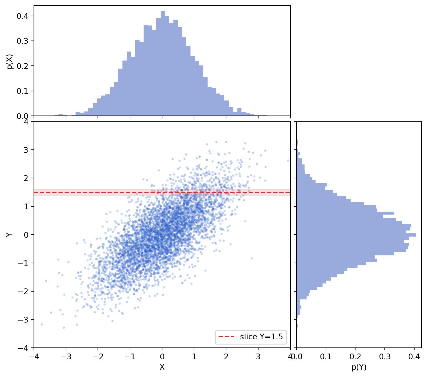
The clearest way to internalize joint, marginal, and conditional structure is to draw samples and look at them. The following implementations sample from the bivariate Gaussian of the worked example, with zero mean, unit variances, and correlation \(\rho = 0.7\). They report the empirical covariance matrix and correlation, compare an empirical conditional slice \(X \mid Y \approx y_0\) against the analytic prediction of mean \(\rho\, y_0\) and standard deviation \(\sqrt{1 - \rho^2}\), and render the joint scatter flanked by the two marginal histograms.
The empirical correlation lands close to \(0.7\), and the slice statistics track the analytic conditional mean \(\rho\, y_0 = 1.05\) and standard deviation \(\sqrt{1 - 0.49} \approx 0.714\), confirming the closed-form conditioning rule on real samples.
// Illustrative: requires the `rand` and `rand_distr` crates.// Cholesky of [[1, rho], [rho, 1]] transforms standard normals into// correlated samples, then we summarize the empirical correlation.userand::SeedableRng;userand::rngs::StdRng;userand_distr::{Distribution, StandardNormal};fn main() {let rho:f64=0.7;letmut rng =StdRng::seed_from_u64(30);// Cholesky factor L of the covariance: L = [[1, 0], [rho, sqrt(1 - rho^2)]].let l21 = rho;let l22 = (1.0- rho * rho).sqrt();let n =5000;letmut xs =Vec::with_capacity(n);letmut ys =Vec::with_capacity(n);for _ in0..n {let z1:f64= StandardNormal.sample(&mut rng);let z2:f64= StandardNormal.sample(&mut rng);// x = z1; y = L * z, second row. xs.push(z1); ys.push(l21 * z1 + l22 * z2);}let mean =|v:&[f64]| v.iter().sum::<f64>() / v.len() asf64;let mx = mean(&xs);let my = mean(&ys);let cov:f64= xs.iter().zip(&ys).map(|(a, b)| (a - mx) * (b - my)).sum::<f64>()/ n asf64;let vx:f64= xs.iter().map(|a| (a - mx).powi(2)).sum::<f64>() / n asf64;let vy:f64= ys.iter().map(|b| (b - my).powi(2)).sum::<f64>() / n asf64;println!("empirical correlation: {:.3} (true rho = {})", cov / (vx.sqrt() * vy.sqrt()), rho);// Analytic conditional X | Y = y0.let y0 =1.5_f64;println!("conditional X | Y={}: mean = {:.3}, std = {:.3}", y0, rho * y0, (1.0- rho * rho).sqrt());}
The Julia version leans on the Distributions.jlMvNormal type, while the Rust version makes the correlation structure explicit through a Cholesky factor: drawing independent standard normals and applying the lower-triangular factor \(\mathbf{L}\) of \(\boldsymbol{\Sigma}\) yields samples with exactly the target covariance, since \(\operatorname{Cov}(\mathbf{L}\mathbf{z}) = \mathbf{L}\,\mathbf{L}^\top = \boldsymbol{\Sigma}\) when \(\mathbf{z}\) has identity covariance.
34.9 References
Bishop, C. M. (2006). Pattern Recognition and Machine Learning. Springer. ISBN 978-0387310732. https://link.springer.com/book/9780387310732
Murphy, K. P. (2022). Probabilistic Machine Learning: An Introduction. MIT Press. ISBN 978-0262046824. https://probml.github.io/pml-book/book1.html
Goodfellow, I., Bengio, Y., and Courville, A. (2016). Deep Learning. MIT Press. ISBN 978-0262035613. https://www.deeplearningbook.org/
Deisenroth, M. P., Faisal, A. A., and Ong, C. S. (2020). Mathematics for Machine Learning. Cambridge University Press. https://doi.org/10.1017/9781108679930
Wasserman, L. (2004). All of Statistics: A Concise Course in Statistical Inference. Springer. https://doi.org/10.1007/978-0-387-21736-9
Eaton, M. L. (2007). Multivariate Statistics: A Vector Space Approach. Institute of Mathematical Statistics Lecture Notes. https://doi.org/10.1214/lnms/1196285102
van den Oord, A., Kalchbrenner, N., and Kavukcuoglu, K. (2016). Pixel Recurrent Neural Networks. Proceedings of the 33rd International Conference on Machine Learning (ICML), PMLR 48:1747-1756. https://doi.org/10.48550/arXiv.1601.06759
Source Code
# Joint, Marginal, and Conditional DistributionsMost interesting questions in machine learning involve more than one random variable at a time. A classifier reasons about a label given an image, a language model predicts a token given a context, and a recommender system models the relationship between users and items. The mathematical machinery that lets us describe how several random variables behave together, and how knowledge of some informs our beliefs about others, is the theory of joint, marginal, and conditional distributions. This chapter develops that machinery in depth, builds up to the chain rule of probability, and then studies the second-order structure captured by covariance and correlation. We close with a detailed treatment of the multivariate Gaussian, the single most important distribution in applied statistics and machine learning.## 1. Joint Distributions### 1.1 Defining the Joint DistributionConsider two random variables $X$ and $Y$ defined on the same probability space. The joint distribution describes the probability of events involving both variables simultaneously. In the discrete case, the joint probability mass function (PMF) is$$p_{X,Y}(x, y) = P(X = x, Y = y),$$where the comma denotes logical conjunction, so we are asking for the probability that $X = x$ and $Y = y$ both hold. A valid joint PMF satisfies $p_{X,Y}(x,y) \ge 0$ for all pairs and sums to one,$$\sum_{x} \sum_{y} p_{X,Y}(x, y) = 1.$$In the continuous case, the joint probability density function (PDF) $f_{X,Y}(x,y)$ plays the analogous role, with probabilities recovered by integration over regions:$$P\big((X, Y) \in A\big) = \iint_{A} f_{X,Y}(x, y)\, dx\, dy,$$and the normalization condition becomes a double integral over the whole plane equal to one. The density itself is not a probability; it is a probability per unit area, and it may exceed one as long as the integral is well behaved.### 1.2 Why Joint Structure MattersThe joint distribution carries strictly more information than the two variables considered separately. Knowing how often it rains and knowing how often the ground is wet does not tell you whether those two facts move together, but the joint distribution does. In machine learning we frequently posit a joint distribution $p(x, y)$ over inputs $x$ and labels $y$, and the entire supervised learning enterprise can be framed as trying to learn useful properties of that joint object from a finite sample. Generative models such as variational autoencoders and diffusion models go further and attempt to model the full joint density of high-dimensional data directly.For a vector of $d$ random variables collected into $\mathbf{X} = (X_1, \ldots, X_d)$, the joint distribution lives in a $d$-dimensional space. The number of parameters needed to specify an arbitrary joint distribution grows exponentially with $d$, a phenomenon known as the curse of dimensionality. Much of probabilistic modeling consists of imposing structure, such as independence or conditional independence, to make the joint tractable.## 2. Marginalization### 2.1 From Joint to MarginalGiven a joint distribution, we often want the distribution of a single variable, ignoring the others. This is the marginal distribution, and the operation that produces it is marginalization. For discrete variables we sum out the variable we wish to discard:$$p_X(x) = \sum_{y} p_{X,Y}(x, y).$$For continuous variables we integrate it out:$$f_X(x) = \int_{-\infty}^{\infty} f_{X,Y}(x, y)\, dy.$$The name comes from a historical practice of writing the row sums and column sums of a tabulated joint distribution in the margins of the table. Marginalization is the probabilistic analogue of projection. We collapse a higher-dimensional object onto a lower-dimensional one by integrating away the directions we do not care about.### 2.2 Marginalization in PracticeMarginalization is everywhere in machine learning, and it is frequently the hard part. The evidence in Bayesian inference,$$p(x) = \int p(x \mid \theta)\, p(\theta)\, d\theta,$$is a marginal obtained by integrating the joint over all parameter values. When we have latent variables $z$, the likelihood of an observation requires marginalizing them out,$$p(x) = \int p(x, z)\, dz = \int p(x \mid z)\, p(z)\, dz,$$and this integral is intractable for most interesting models. Techniques such as variational inference and Monte Carlo sampling exist precisely because exact marginalization is so often impossible. A key conceptual point is that marginalization respects nothing about the structure of the discarded variable; it simply averages over all of its possible values, weighted by their probability.## 3. Conditional Distributions### 3.1 The Definition of ConditioningConditioning answers the question: given that I have observed one variable take a particular value, what is the distribution of another? The conditional PMF or PDF is defined as the ratio of the joint to the marginal,$$p_{Y \mid X}(y \mid x) = \frac{p_{X,Y}(x, y)}{p_X(x)}, \qquad f_{Y \mid X}(y \mid x) = \frac{f_{X,Y}(x, y)}{f_X(x)},$$defined wherever the marginal in the denominator is nonzero. Dividing by the marginal renormalizes the slice of the joint at $X = x$ so that it integrates to one as a proper distribution over $y$. Geometrically, fixing $X = x$ selects a one-dimensional slice through the joint density, and the division rescales that slice so that it becomes a valid distribution in its own right.Rearranging the definition gives the product rule, the foundation for nearly everything that follows:$$p_{X,Y}(x, y) = p_{Y \mid X}(y \mid x)\, p_X(x) = p_{X \mid Y}(x \mid y)\, p_Y(y).$$### 3.2 Independence and Conditional IndependenceTwo variables are independent when conditioning on one does not change the distribution of the other, which is equivalent to the joint factoring as the product of marginals,$$p_{X,Y}(x, y) = p_X(x)\, p_Y(y) \quad \text{for all } x, y.$$A weaker and far more useful notion is conditional independence. We say $X$ and $Y$ are conditionally independent given $Z$, written $X \perp Y \mid Z$, when$$p_{X,Y \mid Z}(x, y \mid z) = p_{X \mid Z}(x \mid z)\, p_{Y \mid Z}(y \mid z).$$Conditional independence is the cornerstone of probabilistic graphical models. The naive Bayes classifier assumes that features are conditionally independent given the class label, which collapses an intractable joint over features into a simple product. Bayesian networks encode a web of conditional independence assumptions as a directed graph, and those assumptions are exactly what make inference and learning feasible.### 3.3 Bayes' TheoremEquating the two factorizations of the joint and solving for one conditional yields Bayes' theorem,$$p_{X \mid Y}(x \mid y) = \frac{p_{Y \mid X}(y \mid x)\, p_X(x)}{p_Y(y)},$$where the denominator is the marginal $p_Y(y) = \sum_x p_{Y \mid X}(y \mid x)\, p_X(x)$ obtained by marginalization. This deceptively simple identity is the engine of Bayesian machine learning. It tells us how to invert a conditional, turning a model of how data arise given parameters into a posterior belief about parameters given data. The prior $p_X(x)$, the likelihood $p_{Y \mid X}(y \mid x)$, and the evidence $p_Y(y)$ each play a distinct role, and the difficulty of computing the evidence is again a marginalization problem.## 4. The Chain Rule of Probability### 4.1 Factorizing a Joint DistributionThe product rule for two variables generalizes to any number of variables. Applying it repeatedly, any joint distribution over $X_1, \ldots, X_n$ factorizes as a product of conditionals:$$p(x_1, x_2, \ldots, x_n) = p(x_1)\, p(x_2 \mid x_1)\, p(x_3 \mid x_1, x_2) \cdots p(x_n \mid x_1, \ldots, x_{n-1}).$$More compactly,$$p(x_1, \ldots, x_n) = \prod_{i=1}^{n} p\big(x_i \mid x_1, \ldots, x_{i-1}\big).$$This is the chain rule of probability. It holds for any ordering of the variables and requires no assumptions whatsoever; it is a pure consequence of the definition of conditional probability. Different orderings give different but equally valid factorizations, and choosing a convenient ordering is often where modeling insight enters.### 4.2 The Chain Rule in Modern Machine LearningThe chain rule underwrites autoregressive modeling, which is the paradigm behind large language models. A language model treats a sentence as a sequence of tokens and factorizes the joint probability of the sequence left to right,$$p(w_1, \ldots, w_T) = \prod_{t=1}^{T} p\big(w_t \mid w_1, \ldots, w_{t-1}\big),$$so that generating text reduces to repeatedly sampling the next token from a learned conditional. Each conditional $p(w_t \mid w_{<t})$ is computed by a neural network, and training maximizes the log probability the chain rule assigns to observed sequences. The same logic drives autoregressive image models such as PixelRNN and the autoregressive components of many other generative architectures. When conditional independence assumptions are layered on top of the chain rule, the long conditioning contexts shrink, and we recover the compact factorizations of graphical models. The chain rule, then, is the bridge between raw probability theory and the structured probabilistic models that dominate the field.## 5. Covariance and Correlation### 5.1 CovarianceWhile the full joint distribution captures all dependence, we often summarize the linear part of that dependence with a single number. The covariance of two random variables measures how they vary together,$$\operatorname{Cov}(X, Y) = \mathbb{E}\big[(X - \mu_X)(Y - \mu_Y)\big] = \mathbb{E}[XY] - \mathbb{E}[X]\,\mathbb{E}[Y],$$where $\mu_X = \mathbb{E}[X]$ and $\mu_Y = \mathbb{E}[Y]$. A positive covariance means the variables tend to lie on the same side of their means together, a negative covariance means they tend to lie on opposite sides, and a covariance of zero means there is no linear association. The covariance of a variable with itself is its variance, $\operatorname{Cov}(X, X) = \operatorname{Var}(X)$.A crucial subtlety is that independence implies zero covariance, but zero covariance does not imply independence. Two variables can be strongly dependent through a nonlinear relationship while having exactly zero covariance. If $X$ is symmetric about zero and $Y = X^2$, then $X$ and $Y$ are functionally dependent, yet their covariance vanishes. Covariance sees only linear structure.The covariance is bilinear in its arguments, a property worth deriving once because it is used constantly. For constants $a$, $b$, $c$, $d$ and random variables $X$, $Y$, $Z$,$$\operatorname{Cov}(aX + b,\; cY + d) = ac\, \operatorname{Cov}(X, Y).$$To see this, note that adding constants does not change the deviations from the mean, since $\mathbb{E}[aX + b] = a\,\mathbb{E}[X] + b$, so $(aX + b) - \mathbb{E}[aX + b] = a(X - \mu_X)$. Substituting into the definition,$$\operatorname{Cov}(aX + b, cY + d) = \mathbb{E}\big[a(X - \mu_X)\, c(Y - \mu_Y)\big] = ac\, \mathbb{E}\big[(X - \mu_X)(Y - \mu_Y)\big] = ac\, \operatorname{Cov}(X, Y).$$A second key property is additivity, $\operatorname{Cov}(X + Y, Z) = \operatorname{Cov}(X, Z) + \operatorname{Cov}(Y, Z)$, which follows from the linearity of expectation applied to the deviation products. Combining bilinearity with the identity $\operatorname{Cov}(X, X) = \operatorname{Var}(X)$ gives the variance of a sum,$$\operatorname{Var}(X + Y) = \operatorname{Var}(X) + \operatorname{Var}(Y) + 2\operatorname{Cov}(X, Y),$$which reduces to the familiar additivity of variances exactly when $X$ and $Y$ are uncorrelated.### 5.2 CorrelationCovariance has the awkward property of carrying the product of the units of $X$ and $Y$, which makes its magnitude hard to interpret. The Pearson correlation coefficient fixes this by normalizing,$$\rho_{X,Y} = \frac{\operatorname{Cov}(X, Y)}{\sigma_X\, \sigma_Y},$$where $\sigma_X$ and $\sigma_Y$ are the standard deviations. The bound $\rho_{X,Y} \in [-1, 1]$ is a direct consequence of the Cauchy-Schwarz inequality, which we can derive cleanly. Center the variables as $U = X - \mu_X$ and $V = Y - \mu_Y$, and consider the nonnegative quantity $\mathbb{E}\big[(tU + V)^2\big] \ge 0$ for every real $t$. Expanding,$$\mathbb{E}\big[(tU + V)^2\big] = t^2\, \mathbb{E}[U^2] + 2t\, \mathbb{E}[UV] + \mathbb{E}[V^2] \ge 0.$$This is a quadratic in $t$ that is never negative, so its discriminant cannot be positive,$$\big(2\,\mathbb{E}[UV]\big)^2 - 4\, \mathbb{E}[U^2]\, \mathbb{E}[V^2] \le 0 \quad\Longrightarrow\quad \big(\operatorname{Cov}(X, Y)\big)^2 \le \operatorname{Var}(X)\, \operatorname{Var}(Y),$$since $\mathbb{E}[UV] = \operatorname{Cov}(X, Y)$, $\mathbb{E}[U^2] = \operatorname{Var}(X)$, and $\mathbb{E}[V^2] = \operatorname{Var}(Y)$. Dividing both sides by $\sigma_X^2 \sigma_Y^2$ yields $\rho_{X,Y}^2 \le 1$. Equality holds exactly when $tU + V = 0$ almost surely for some $t$, that is, when $Y$ is an exact linear function of $X$. A value of $+1$ indicates a perfect increasing linear relationship, $-1$ a perfect decreasing one, and $0$ the absence of linear association. Correlation is dimensionless and invariant to separate positive linear rescalings of each variable, which is why it is the standard tool for reporting the strength of an association. In machine learning, feature correlation analysis guides feature selection, flags redundant predictors, and warns of multicollinearity that can destabilize linear models.## 6. The Covariance Matrix### 6.1 Definition and StructureWhen we move from two variables to a random vector $\mathbf{X} = (X_1, \ldots, X_d)^\top$, the pairwise covariances assemble into a matrix. The covariance matrix is$$\boldsymbol{\Sigma} = \operatorname{Cov}(\mathbf{X}) = \mathbb{E}\big[(\mathbf{X} - \boldsymbol{\mu})(\mathbf{X} - \boldsymbol{\mu})^\top\big],$$where $\boldsymbol{\mu} = \mathbb{E}[\mathbf{X}]$ is the mean vector. The entry in row $i$ and column $j$ is $\Sigma_{ij} = \operatorname{Cov}(X_i, X_j)$, so the diagonal holds the variances of the individual components and the off-diagonal entries hold the pairwise covariances. Because $\operatorname{Cov}(X_i, X_j) = \operatorname{Cov}(X_j, X_i)$, the covariance matrix is symmetric.### 6.2 Positive SemidefinitenessBeyond symmetry, every valid covariance matrix is positive semidefinite, meaning that for any constant vector $\mathbf{a} \in \mathbb{R}^d$,$$\mathbf{a}^\top \boldsymbol{\Sigma}\, \mathbf{a} = \operatorname{Var}(\mathbf{a}^\top \mathbf{X}) \ge 0.$$The identity follows because $\mathbf{a}^\top \boldsymbol{\Sigma} \mathbf{a}$ is exactly the variance of the scalar projection $\mathbf{a}^\top \mathbf{X}$, and a variance can never be negative. Positive semidefiniteness guarantees that all eigenvalues of $\boldsymbol{\Sigma}$ are nonnegative, which in turn underpins the spectral decomposition used throughout dimensionality reduction.### 6.3 The Covariance Matrix and Principal Component AnalysisPrincipal component analysis (PCA) is the canonical application of the covariance matrix in machine learning. PCA performs an eigendecomposition of $\boldsymbol{\Sigma}$,$$\boldsymbol{\Sigma} = \mathbf{U}\, \boldsymbol{\Lambda}\, \mathbf{U}^\top,$$where the columns of $\mathbf{U}$ are orthonormal eigenvectors and $\boldsymbol{\Lambda}$ is the diagonal matrix of eigenvalues. The eigenvectors point along the directions of greatest variance in the data, and the corresponding eigenvalues quantify how much variance lies along each direction. Projecting data onto the top few eigenvectors retains most of the variance while discarding noisy or redundant directions, giving a compact representation. The covariance matrix also defines the Mahalanobis distance, $\sqrt{(\mathbf{x} - \boldsymbol{\mu})^\top \boldsymbol{\Sigma}^{-1} (\mathbf{x} - \boldsymbol{\mu})}$, which measures distance in units that account for the spread and correlation of the data, and which appears as the exponent of the multivariate Gaussian.## 7. The Multivariate Gaussian in Depth### 7.1 The DensityThe multivariate Gaussian, or multivariate normal, distribution generalizes the familiar bell curve to $d$ dimensions. A random vector $\mathbf{X} \in \mathbb{R}^d$ is multivariate Gaussian with mean $\boldsymbol{\mu}$ and covariance $\boldsymbol{\Sigma}$, written $\mathbf{X} \sim \mathcal{N}(\boldsymbol{\mu}, \boldsymbol{\Sigma})$, when its density is$$f(\mathbf{x}) = \frac{1}{(2\pi)^{d/2}\, |\boldsymbol{\Sigma}|^{1/2}} \exp\left(-\tfrac{1}{2}(\mathbf{x} - \boldsymbol{\mu})^\top \boldsymbol{\Sigma}^{-1} (\mathbf{x} - \boldsymbol{\mu})\right),$$where $|\boldsymbol{\Sigma}|$ denotes the determinant. The quadratic form in the exponent is the squared Mahalanobis distance, so surfaces of constant density are ellipsoids centered at $\boldsymbol{\mu}$. The eigenvectors of $\boldsymbol{\Sigma}$ give the orientation of those ellipsoids, and the square roots of the eigenvalues give their semi-axis lengths. The normalizing constant out front ensures the density integrates to one, with the determinant measuring the volume of the ellipsoid of concentration.### 7.2 Marginals and ConditionalsThe multivariate Gaussian is special because it is closed under both marginalization and conditioning, and the resulting distributions are again Gaussian with parameters given in closed form. Partition the vector as $\mathbf{X} = (\mathbf{X}_a, \mathbf{X}_b)$ with the mean and covariance blocked conformably,$$\boldsymbol{\mu} = \begin{pmatrix} \boldsymbol{\mu}_a \\ \boldsymbol{\mu}_b \end{pmatrix}, \qquad \boldsymbol{\Sigma} = \begin{pmatrix} \boldsymbol{\Sigma}_{aa} & \boldsymbol{\Sigma}_{ab} \\ \boldsymbol{\Sigma}_{ba} & \boldsymbol{\Sigma}_{bb} \end{pmatrix}.$$The marginal of any sub-vector is read off directly: $\mathbf{X}_a \sim \mathcal{N}(\boldsymbol{\mu}_a, \boldsymbol{\Sigma}_{aa})$. We simply keep the relevant blocks and discard the rest. The conditional is also Gaussian, with mean and covariance$$\boldsymbol{\mu}_{a \mid b} = \boldsymbol{\mu}_a + \boldsymbol{\Sigma}_{ab} \boldsymbol{\Sigma}_{bb}^{-1} (\mathbf{x}_b - \boldsymbol{\mu}_b),$$$$\boldsymbol{\Sigma}_{a \mid b} = \boldsymbol{\Sigma}_{aa} - \boldsymbol{\Sigma}_{ab} \boldsymbol{\Sigma}_{bb}^{-1} \boldsymbol{\Sigma}_{ba}.$$These formulas repay close study. The conditional mean is a linear function of the observed value $\mathbf{x}_b$, which is why linear regression with Gaussian assumptions produces linear predictors. The conditional covariance does not depend on $\mathbf{x}_b$ at all, and it is never larger than the unconditional covariance, capturing the intuition that observing $\mathbf{x}_b$ can only reduce or maintain our uncertainty about $\mathbf{x}_a$. The term $\boldsymbol{\Sigma}_{ab}\boldsymbol{\Sigma}_{bb}^{-1}\boldsymbol{\Sigma}_{ba}$ is the variance explained by the observation.#### Deriving the conditionalThe conditioning formulas are not magic; they fall out of completing the square in the exponent. The cleanest derivation uses the block inverse of $\boldsymbol{\Sigma}$, written in terms of the Schur complement $\mathbf{S} = \boldsymbol{\Sigma}_{aa} - \boldsymbol{\Sigma}_{ab} \boldsymbol{\Sigma}_{bb}^{-1} \boldsymbol{\Sigma}_{ba}$. The inverse covariance, or precision matrix, has the block form$$\boldsymbol{\Sigma}^{-1} = \begin{pmatrix} \mathbf{S}^{-1} & -\mathbf{S}^{-1} \boldsymbol{\Sigma}_{ab} \boldsymbol{\Sigma}_{bb}^{-1} \\ -\boldsymbol{\Sigma}_{bb}^{-1} \boldsymbol{\Sigma}_{ba} \mathbf{S}^{-1} & \boldsymbol{\Sigma}_{bb}^{-1} + \boldsymbol{\Sigma}_{bb}^{-1} \boldsymbol{\Sigma}_{ba} \mathbf{S}^{-1} \boldsymbol{\Sigma}_{ab} \boldsymbol{\Sigma}_{bb}^{-1} \end{pmatrix}.$$The conditional density $f(\mathbf{x}_a \mid \mathbf{x}_b) \propto f(\mathbf{x}_a, \mathbf{x}_b)$ is obtained by holding $\mathbf{x}_b$ fixed and treating the joint density as a function of $\mathbf{x}_a$ alone. The exponent of the joint is the quadratic form $-\tfrac{1}{2}(\mathbf{x} - \boldsymbol{\mu})^\top \boldsymbol{\Sigma}^{-1} (\mathbf{x} - \boldsymbol{\mu})$. Collecting the terms in $\mathbf{x}_a$ and using the top-left block $\mathbf{S}^{-1}$ as the quadratic coefficient, the part of the exponent that depends on $\mathbf{x}_a$ is$$-\tfrac{1}{2}\Big[ \mathbf{x}_a^\top \mathbf{S}^{-1} \mathbf{x}_a - 2\, \mathbf{x}_a^\top \mathbf{S}^{-1}\big(\boldsymbol{\mu}_a + \boldsymbol{\Sigma}_{ab} \boldsymbol{\Sigma}_{bb}^{-1}(\mathbf{x}_b - \boldsymbol{\mu}_b)\big) \Big] + \text{const}.$$Any density whose log is a quadratic with leading matrix $\mathbf{S}^{-1}$ and linear term matching the displayed expression is Gaussian with covariance $\mathbf{S}$ and mean equal to the vector multiplying the linear term. Reading these off gives exactly $\boldsymbol{\Sigma}_{a \mid b} = \mathbf{S}$ and $\boldsymbol{\mu}_{a \mid b} = \boldsymbol{\mu}_a + \boldsymbol{\Sigma}_{ab} \boldsymbol{\Sigma}_{bb}^{-1}(\mathbf{x}_b - \boldsymbol{\mu}_b)$, confirming the formulas above.#### A worked exampleTake the bivariate case with $\boldsymbol{\mu} = (0, 0)^\top$ and$$\boldsymbol{\Sigma} = \begin{pmatrix} 1 & \rho \\ \rho & 1 \end{pmatrix}, \qquad |\rho| < 1,$$so that each component is standard normal with correlation $\rho$. With $a$ indexing the first coordinate and $b$ the second, the scalar blocks are $\Sigma_{aa} = 1$, $\Sigma_{ab} = \Sigma_{ba} = \rho$, and $\Sigma_{bb} = 1$. The conditional of $X_a$ given $X_b = x_b$ is then Gaussian with$$\mu_{a \mid b} = 0 + \rho \cdot 1 \cdot (x_b - 0) = \rho\, x_b, \qquad \sigma^2_{a \mid b} = 1 - \rho \cdot 1 \cdot \rho = 1 - \rho^2.$$The conditional mean $\rho\, x_b$ is the textbook regression line through the origin with slope $\rho$, and the conditional variance $1 - \rho^2$ shows quantitatively how much the observation shrinks our uncertainty: at $\rho = 0$ the variance is unchanged at one, while as $|\rho| \to 1$ it collapses toward zero because $X_a$ becomes nearly determined by $X_b$. The Python cell below samples from exactly this distribution and overlays the analytic conditional slice on the empirical one.### 7.3 Why the Gaussian Dominates Machine LearningSeveral deep properties explain the ubiquity of the Gaussian. The central limit theorem shows that sums of many independent influences tend toward a Gaussian regardless of their individual distributions, which makes the Gaussian a natural model for aggregate noise. Among all distributions with a given mean and covariance, the Gaussian has maximum entropy, so it is the least committal choice consistent with second-order statistics. The closure properties above mean that Gaussian assumptions propagate cleanly through linear operations, which is exactly the structure exploited by the Kalman filter, by Gaussian processes, and by the reparameterization trick in variational autoencoders. Linear-Gaussian models also yield exact, closed-form inference, a rarity in probabilistic modeling that makes them the default building block whenever analytical tractability is needed. When a model needs a flexible yet analytically convenient distribution over continuous vectors, the multivariate Gaussian is almost always the first and often the final answer.### 7.4 Connecting the ThreadsThe Gaussian ties together every concept in this chapter. Its parameters are exactly a mean vector and a covariance matrix, so it is fully specified by first-order and second-order moments. Its marginals are obtained by selecting blocks of the covariance matrix, a clean instance of marginalization. Its conditionals follow from the product rule and inherit the chain rule structure when we factor a joint Gaussian across its components. And its contours are governed by the covariance matrix through the Mahalanobis metric. Mastering the joint, marginal, and conditional view of probability, together with the second-order summary provided by covariance, gives you the complete toolkit for reasoning about the multivariate Gaussian and, by extension, a large fraction of probabilistic machine learning.## 8. Sampling and Visualizing a Bivariate GaussianThe clearest way to internalize joint, marginal, and conditional structure is to draw samples and look at them. The following implementations sample from the bivariate Gaussian of the worked example, with zero mean, unit variances, and correlation $\rho = 0.7$. They report the empirical covariance matrix and correlation, compare an empirical conditional slice $X \mid Y \approx y_0$ against the analytic prediction of mean $\rho\, y_0$ and standard deviation $\sqrt{1 - \rho^2}$, and render the joint scatter flanked by the two marginal histograms.::: {.panel-tabset}## Python executable```{python}import numpy as npimport matplotlib.pyplot as pltfrom matplotlib.gridspec import GridSpecrng = np.random.default_rng(30)# Bivariate Gaussian: zero mean, unit variances, correlation rho.rho =0.7mu = np.array([0.0, 0.0])Sigma = np.array([[1.0, rho], [rho, 1.0]])# Draw samples.n =5000samples = rng.multivariate_normal(mu, Sigma, size=n)x, y = samples[:, 0], samples[:, 1]# Empirical second-order summary, compared with the truth.emp_cov = np.cov(samples, rowvar=False)emp_corr = np.corrcoef(samples, rowvar=False)[0, 1]print("empirical covariance matrix:")print(np.round(emp_cov, 3))print(f"empirical correlation: {emp_corr:.3f} (true rho = {rho})")# Analytic conditional of X given Y = y0: mean rho*y0, variance 1 - rho^2.y0 =1.5cond_mean = rho * y0cond_std = np.sqrt(1.0- rho **2)print(f"\nconditional X | Y={y0}: mean = {cond_mean:.3f}, std = {cond_std:.3f}")# Empirical conditional slice: samples whose y falls in a thin band around y0.band =0.1mask = np.abs(y - y0) < bandx_slice = x[mask]print(f"samples in slice |Y - {y0}| < {band}: {mask.sum()}")print(f"empirical slice mean = {x_slice.mean():.3f}, std = {x_slice.std():.3f}")# Joint scatter with marginal histograms and the conditioning band.fig = plt.figure(figsize=(9, 8))gs = GridSpec(3, 3, figure=fig, hspace=0.05, wspace=0.05)ax_main = fig.add_subplot(gs[1:3, 0:2])ax_top = fig.add_subplot(gs[0, 0:2], sharex=ax_main)ax_right = fig.add_subplot(gs[1:3, 2], sharey=ax_main)ax_main.scatter(x, y, s=4, alpha=0.2, color="#3366cc")ax_main.axhline(y0, color="#cc3333", lw=1.5, ls="--", label=f"slice Y={y0}")ax_main.fill_between([-4, 4], y0 - band, y0 + band, color="#cc3333", alpha=0.15)ax_main.set_xlim(-4, 4)ax_main.set_ylim(-4, 4)ax_main.set_xlabel("X")ax_main.set_ylabel("Y")ax_main.legend(loc="lower right")ax_top.hist(x, bins=60, density=True, color="#99aadd")ax_top.set_ylabel("p(X)")ax_top.tick_params(labelbottom=False)ax_right.hist(y, bins=60, density=True, orientation="horizontal", color="#99aadd")ax_right.set_xlabel("p(Y)")ax_right.tick_params(labelleft=False)plt.show()```The empirical correlation lands close to $0.7$, and the slice statistics track the analytic conditional mean $\rho\, y_0 = 1.05$ and standard deviation $\sqrt{1 - 0.49} \approx 0.714$, confirming the closed-form conditioning rule on real samples.## Julia```juliausingRandom, Distributions, Statistics, PlotsRandom.seed!(30)# Bivariate Gaussian: zero mean, unit variances, correlation rho.rho =0.7mu = [0.0, 0.0]Sigma = [1.0 rho; rho 1.0]dist =MvNormal(mu, Sigma)# Draw samples (columns are observations).n =5000samples =rand(dist, n)x = samples[1, :]y = samples[2, :]# Empirical second-order summary.println("empirical covariance matrix:")println(round.(cov(samples; dims =2), digits =3))println("empirical correlation: ", round(cor(x, y), digits =3), " (true rho = ", rho, ")")# Analytic conditional of X given Y = y0.y0 =1.5cond_mean = rho * y0cond_std =sqrt(1.0- rho^2)println("conditional X | Y=", y0, ": mean = ", round(cond_mean, digits =3),", std = ", round(cond_std, digits =3))# Empirical conditional slice.band =0.1slice = x[abs.(y .- y0) .< band]println("empirical slice mean = ", round(mean(slice), digits =3),", std = ", round(std(slice), digits =3))scatter(x, y; markersize =1, alpha =0.2, legend =false, xlabel ="X", ylabel ="Y", xlims = (-4, 4), ylims = (-4, 4))hline!([y0]; color =:red, linestyle =:dash)```## Rust```rust// Illustrative: requires the `rand` and `rand_distr` crates.// Cholesky of [[1, rho], [rho, 1]] transforms standard normals into// correlated samples, then we summarize the empirical correlation.use rand::SeedableRng;use rand::rngs::StdRng;use rand_distr::{Distribution, StandardNormal};fn main() { let rho: f64 =0.7; let mut rng = StdRng::seed_from_u64(30);// Cholesky factor L of the covariance: L = [[1, 0], [rho, sqrt(1- rho^2)]]. let l21 = rho; let l22 = (1.0- rho * rho).sqrt(); let n =5000; let mut xs = Vec::with_capacity(n); let mut ys = Vec::with_capacity(n);for _ in0..n { let z1: f64 =StandardNormal.sample(&mut rng); let z2: f64 =StandardNormal.sample(&mut rng);// x = z1; y = L * z, second row.xs.push(z1);ys.push(l21 * z1 + l22 * z2); } let mean =|v:&[f64]|v.iter().sum::<f64>() /v.len() as f64; let mx =mean(&xs); let my =mean(&ys); let cov: f64 =xs.iter().zip(&ys).map(|(a, b)| (a - mx) * (b - my)).sum::<f64>()/ n as f64; let vx: f64 =xs.iter().map(|a| (a - mx).powi(2)).sum::<f64>() / n as f64; let vy: f64 =ys.iter().map(|b| (b - my).powi(2)).sum::<f64>() / n as f64; println!("empirical correlation: {:.3} (true rho = {})", cov / (vx.sqrt() *vy.sqrt()), rho);// Analytic conditional X | Y = y0. let y0 =1.5_f64; println!("conditional X | Y={}: mean = {:.3}, std = {:.3}", y0, rho * y0, (1.0- rho * rho).sqrt());}```:::The Julia version leans on the `Distributions.jl``MvNormal` type, while the Rust version makes the correlation structure explicit through a Cholesky factor: drawing independent standard normals and applying the lower-triangular factor $\mathbf{L}$ of $\boldsymbol{\Sigma}$ yields samples with exactly the target covariance, since $\operatorname{Cov}(\mathbf{L}\mathbf{z}) = \mathbf{L}\,\mathbf{L}^\top = \boldsymbol{\Sigma}$ when $\mathbf{z}$ has identity covariance.## References1. Bishop, C. M. (2006). *Pattern Recognition and Machine Learning*. Springer. ISBN 978-0387310732. https://link.springer.com/book/97803873107322. Murphy, K. P. (2022). *Probabilistic Machine Learning: An Introduction*. MIT Press. ISBN 978-0262046824. https://probml.github.io/pml-book/book1.html3. Goodfellow, I., Bengio, Y., and Courville, A. (2016). *Deep Learning*. MIT Press. ISBN 978-0262035613. https://www.deeplearningbook.org/4. Deisenroth, M. P., Faisal, A. A., and Ong, C. S. (2020). *Mathematics for Machine Learning*. Cambridge University Press. https://doi.org/10.1017/97811086799305. Wasserman, L. (2004). *All of Statistics: A Concise Course in Statistical Inference*. Springer. https://doi.org/10.1007/978-0-387-21736-96. Eaton, M. L. (2007). *Multivariate Statistics: A Vector Space Approach*. Institute of Mathematical Statistics Lecture Notes. https://doi.org/10.1214/lnms/11962851027. van den Oord, A., Kalchbrenner, N., and Kavukcuoglu, K. (2016). Pixel Recurrent Neural Networks. *Proceedings of the 33rd International Conference on Machine Learning (ICML)*, PMLR 48:1747-1756. https://doi.org/10.48550/arXiv.1601.06759