152  Isolation Forests

Anomaly detection has historically been framed as a problem of describing normality. Density estimators, distance based methods, and one class classifiers all build a model of what typical data looks like, then flag points that deviate. Isolation Forests, introduced by Liu, Ting, and Zhou in 2008, invert this logic. Instead of profiling normal points and treating anomalies as residual, the method targets anomalies directly. The insight is deceptively simple. Anomalies are few and different, so they are easy to separate from the rest of the data. This chapter develops the isolation principle, the random partitioning mechanism, the path length statistic, the anomaly score, the extended variant that fixes a geometric flaw, and the computational properties that make the method attractive at scale.

152.1 1. The Isolation Principle

Consider the task of separating a single point from a dataset by recursively cutting the feature space with random splits. A point that sits in a dense region requires many cuts before it ends up alone in its own partition, because each cut must carve through the surrounding crowd of similar points. A point that sits far from the mass of the data, or that has an unusual value on some attribute, gets isolated quickly. A single fortunate cut can place it in a partition by itself.

This is the entire conceptual core. Isolation is susceptibility to separation. Anomalies, being rare and distinct, are more susceptible. The method does not compute distances, does not estimate densities, and does not assume any parametric form for the data. It exploits a structural property: that outliers occupy sparse regions where random cuts isolate them with few operations.

Formally, we measure susceptibility through path length. If we build a binary tree by recursively partitioning the data, the path length \(h(x)\) of a point \(x\) is the number of edges traversed from the root to the external node where \(x\) comes to rest. Anomalies tend to have short path lengths. Normal points tend to have long ones. The job of the algorithm is to estimate the expected path length of each point across many randomly constructed trees and convert it into a calibrated score.

152.2 2. Random Partitioning and Tree Construction

An Isolation Tree, or iTree, is built by recursive random partitioning. Given a sample of data, the procedure selects a feature uniformly at random, then selects a split value uniformly at random between the minimum and maximum observed values of that feature within the current node. The data is partitioned into two children by the split, and the procedure recurses on each child.

import numpy as np

rng = np.random.default_rng(0)


class ExternalNode:
    def __init__(self, size):
        self.size = size


class InternalNode:
    def __init__(self, q, p, left, right):
        self.q, self.p, self.left, self.right = q, p, left, right


def build_itree(X, depth, limit, rng):
    if depth >= limit or X.shape[0] <= 1:
        return ExternalNode(size=X.shape[0])
    q = rng.integers(X.shape[1])
    lo, hi = X[:, q].min(), X[:, q].max()
    if lo == hi:
        return ExternalNode(size=X.shape[0])
    p = rng.uniform(lo, hi)
    left = X[X[:, q] < p]
    right = X[X[:, q] >= p]
    return InternalNode(q, p,
                        build_itree(left, depth + 1, limit, rng),
                        build_itree(right, depth + 1, limit, rng))


def c(n):
    if n <= 1:
        return 0.0
    H = np.log(n - 1) + 0.5772156649  # harmonic number approximation
    return 2.0 * H - 2.0 * (n - 1) / n


def path_length(x, node, depth=0):
    if isinstance(node, ExternalNode):
        return depth + c(node.size)
    if x[node.q] < node.p:
        return path_length(x, node.left, depth + 1)
    return path_length(x, node.right, depth + 1)


psi = 256
normal = rng.normal(0, 1, size=(psi, 2))
limit = int(np.ceil(np.log2(psi)))
tree = build_itree(normal, 0, limit, rng)

center = np.array([0.0, 0.0])
outlier = np.array([6.0, 6.0])
print("path length, center point :", round(path_length(center, tree), 3))
print("path length, far outlier  :", round(path_length(outlier, tree), 3))
print("normalizing constant c(psi):", round(c(psi), 3))

path length, center point : 12.278
path length, far outlier  : 5.0
normalizing constant c(psi): 10.245

Two design choices matter. First, each tree is built from a small subsample of the data rather than the full dataset. The original work recommends a subsampling size of \(\psi = 256\). This is not merely an efficiency hack. Small samples reduce two pathologies known as swamping and masking. Swamping occurs when normal points adjacent to a cluster of anomalies are themselves flagged. Masking occurs when a dense cluster of anomalies hides them from isolation. A small sample thins out the data so that anomalies remain sparse and separable rather than forming clusters that resist isolation.

Second, the recursion is capped at a height limit. Because anomalies are isolated near the top of the tree, there is no value in growing branches deep into the normal data. The height limit is set to \(\lceil \log_2 \psi \rceil\), the average height of a tree built on \(\psi\) points, since paths longer than this carry little discriminative information about anomalies.

An Isolation Forest is an ensemble of \(t\) such trees, each built on an independent subsample. The original work uses \(t = 100\). Averaging over the ensemble smooths the variance introduced by random feature and split selection, yielding a stable estimate of expected path length.

152.3 3. Path Length and Its Normalization

The raw path length is not directly comparable across datasets of different sizes, because the expected depth of a tree grows with the number of points it contains. To make path lengths interpretable we normalize against the expected path length of an unsuccessful search in a Binary Search Tree, which has the same recursive structure as a random partition.

The expected path length for a node containing \(n\) points is

\[ c(n) = 2 H(n - 1) - \frac{2(n - 1)}{n}, \]

where \(H(i)\) is the \(i\)th harmonic number, well approximated by \(H(i) \approx \ln(i) + 0.5772156649\) (the Euler Mascheroni constant). The term \(c(n)\) serves as a normalizing constant: it is the average path length we would expect a typical point to traverse in a tree of \(n\) points.

When a point reaches an external node before the tree is fully grown, because of the height limit or because the node still holds several points, we do not know its exact isolation depth. We estimate it by adding \(c(\text{node size})\) to the path length accumulated so far. This correction accounts for the depth the point would have reached had partitioning continued.

The estimated path length for a point is therefore

\[ h(x) = e + c(\text{size of terminal node}), \]

where \(e\) is the number of edges traversed to reach the terminal node. Averaging \(h(x)\) over all \(t\) trees gives \(E[h(x)]\), the quantity that drives the score.

152.4 4. The Anomaly Score

We want a score that is bounded, monotone in isolation susceptibility, and comparable across datasets. The Isolation Forest score for a point \(x\) over a dataset of subsample size \(\psi\) is

\[ s(x, \psi) = 2^{-\frac{E[h(x)]}{c(\psi)}}. \]

The construction normalizes the expected path length by \(c(\psi)\), the expected path length of a random point, then maps it through an exponential into the unit interval. The behavior at the extremes clarifies the design.

When \(E[h(x)] \to 0\), the point is isolated immediately, and \(s \to 1\). These are the clearest anomalies.

When \(E[h(x)] \to \psi - 1\), the point required maximal partitioning, and \(s \to 0\). These are deeply embedded normal points.

When \(E[h(x)] \to c(\psi)\), the point has an average path length, and \(s \to 0.5\). The point is neither clearly anomalous nor clearly normal.

This gives a clean interpretation rule. Scores well above \(0.5\) indicate anomalies. Scores well below \(0.5\) indicate normal points. A whole dataset whose scores cluster near \(0.5\) suggests no clear anomalies are present. The score is dimensionless and dataset agnostic, which is why a single threshold such as \(s > 0.6\) can carry across problems where raw distances or densities would not.

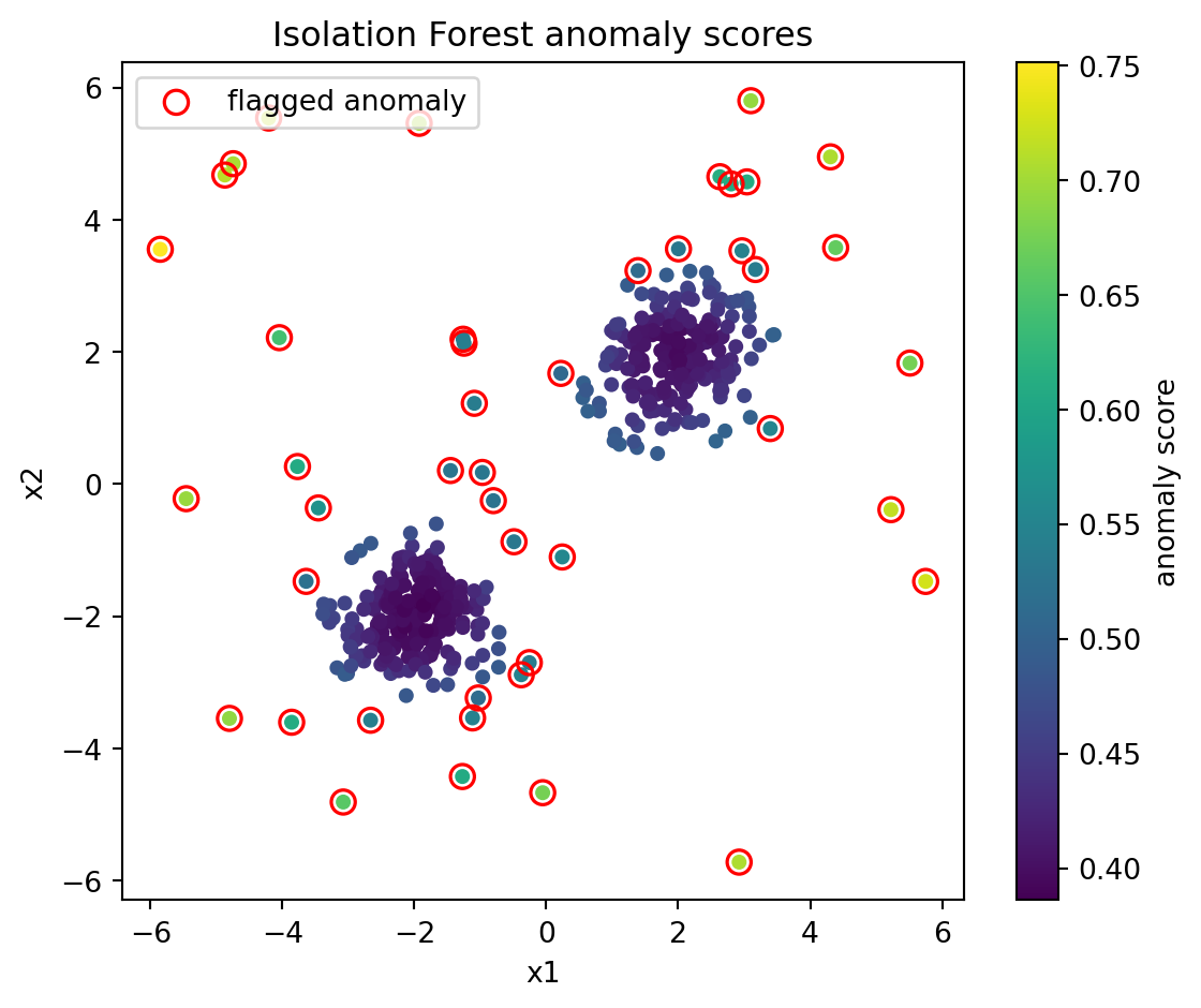
import matplotlib.pyplot as plt
from sklearn.ensemble import IsolationForest

rng = np.random.default_rng(42)

# Two Gaussian blobs as normal data, plus injected uniform outliers.
blob_a = rng.normal(loc=[-2, -2], scale=0.6, size=(200, 2))
blob_b = rng.normal(loc=[2, 2], scale=0.6, size=(200, 2))
inliers = np.vstack([blob_a, blob_b])
outliers = rng.uniform(low=-6, high=6, size=(40, 2))
X = np.vstack([inliers, outliers])

forest = IsolationForest(
    n_estimators=100, max_samples=256, contamination=0.1, random_state=0
)
forest.fit(X)

# score_samples is higher for normal points; negate so larger means more anomalous.
anomaly_score = -forest.score_samples(X)
labels = forest.predict(X)  # -1 anomaly, 1 inlier

print("points:", X.shape[0], "flagged as anomalies:", int((labels == -1).sum()))
print("score range:", round(anomaly_score.min(), 3), "to", round(anomaly_score.max(), 3))

fig, ax = plt.subplots(figsize=(6, 5))
sc = ax.scatter(X[:, 0], X[:, 1], c=anomaly_score, cmap="viridis", s=18)
flagged = labels == -1
ax.scatter(
    X[flagged, 0], X[flagged, 1],
    facecolors="none", edgecolors="red", s=70, linewidths=1.2,
    label="flagged anomaly",
)
fig.colorbar(sc, ax=ax, label="anomaly score")
ax.set_title("Isolation Forest anomaly scores")
ax.set_xlabel("x1")
ax.set_ylabel("x2")
ax.legend(loc="upper left")
plt.tight_layout()
plt.show()

points: 440 flagged as anomalies: 44
score range: 0.386 to 0.751

In practice the score is often used to rank points rather than to apply a hard threshold. Ranking sidesteps the question of where to draw the line and instead surfaces the top \(k\) most isolated points for human review or downstream action, which is how anomaly detection is usually consumed in operational settings.

152.5 5. The Extended Isolation Forest

The standard Isolation Forest has a geometric weakness rooted in the way it cuts. Every split is axis parallel, since each cut fixes a single feature and a threshold on it. The decision boundaries are therefore unions of axis aligned hyperrectangles. This produces an artifact in the score field.

Consider data drawn from a single Gaussian blob centered at the origin. We would expect the anomaly score to be radially symmetric, with low scores near the center rising smoothly outward in every direction. The axis parallel cuts instead produce score contours with spurious structure. Regions aligned with the coordinate axes through the center receive artificially low scores, creating a ghostly cross or rectangular pattern of low score bands extending along the axes even into regions that are genuinely sparse. Points that lie far from the data along a diagonal can receive lower anomaly scores than they should, because the axis aligned splits cannot efficiently isolate them.

The Extended Isolation Forest, proposed by Hariri, Kind, and Brunner in 2019, removes this bias by replacing axis parallel cuts with cuts along random hyperplanes of arbitrary orientation. At each internal node the split is defined by a random normal vector \(\mathbf{n}\) and an intercept point \(\mathbf{p}\). A point \(x\) goes left or right according to the sign of

\[ (\mathbf{x} - \mathbf{p}) \cdot \mathbf{n} \le 0. \]

The normal vector \(\mathbf{n}\) has each coordinate drawn from a standard normal distribution, giving a uniformly random orientation, and \(\mathbf{p}\) is drawn uniformly from the range of the data in the node. The standard Isolation Forest is recovered as the special case where \(\mathbf{n}\) has exactly one nonzero coordinate.

The method admits an extension level parameter that controls how many coordinates of \(\mathbf{n}\) are allowed to be nonzero, interpolating between fully axis parallel (\(1\) nonzero coordinate) and fully unconstrained (all coordinates nonzero). In \(d\) dimensions the extension level ranges from \(0\) to \(d - 1\). Lowering the extension level can be useful when only a subset of dimensions should participate in the splits, or when the axis aligned inductive bias is actually appropriate for the data.

The benefit is that the score field becomes smooth and approximately radial for radially symmetric data, eliminating the artifact bands. The cost is modest. Each split now evaluates a dot product over the active coordinates rather than a single comparison, and the per node storage grows with the dimensionality of the normal vector. For most datasets this overhead is negligible relative to the gain in score fidelity, and the Extended Isolation Forest is now a common default.

152.6 6. Why It Scales Well

The computational appeal of the Isolation Forest follows from the subsampling and the height limit. Consider training cost. Each tree is built on a subsample of fixed size \(\psi\) that does not grow with the dataset. The work to build one tree is therefore \(O(\psi \log \psi)\), independent of the total number of points \(N\). The forest of \(t\) trees costs

\[ O(t \, \psi \log \psi), \]

which is constant with respect to \(N\). This is unusual. Most anomaly detectors that rely on distances or densities pay at least \(O(N^2)\) for pairwise comparisons or \(O(N \log N)\) for spatial index construction over the full data, with poor behavior in high dimensions. The Isolation Forest decouples training cost from dataset size entirely.

Scoring a point requires traversing each of the \(t\) trees to a terminal node. Because every tree is capped at height \(O(\log \psi)\), scoring one point costs \(O(t \log \psi)\), and scoring all \(N\) points costs

\[ O(N \, t \log \psi). \]

This is linear in \(N\), with a small constant since both \(t\) and \(\log \psi\) are modest. Memory is similarly bounded. The whole forest stores \(t\) trees of at most \(2\psi\) nodes each, so the model footprint is \(O(t \, \psi)\) regardless of how much data it eventually scores.

These properties make the method well suited to streaming and high volume settings. A forest trained on a few hundred sampled points can score millions of incoming records cheaply, and because training cost is independent of \(N\), periodic retraining on fresh subsamples to handle distribution drift is inexpensive. The trees are also embarrassingly parallel, both to build and to evaluate, so the wall clock cost falls nearly linearly with available cores.

A few practical caveats temper the optimism. The method assumes anomalies are genuinely sparse and separable. When anomalies form dense local clusters, masking can defeat isolation even with subsampling. The axis parallel variant inherits the geometric artifacts of Section 5, so the extended variant is preferable when score geometry matters. And like all unsupervised detectors, the Isolation Forest finds statistical outliers, which are not always the semantically interesting anomalies a domain expert cares about. The score answers the question of which points are easy to isolate, and whether that coincides with the events worth flagging is a modeling judgment that the algorithm cannot make on its own.

152.7 7. Summary

The Isolation Forest reframes anomaly detection around separability rather than density. Random partitioning produces short path lengths for anomalies and long ones for normal points, the harmonic normalization makes path lengths comparable, and the exponential score maps them into a bounded and interpretable range. The Extended Isolation Forest repairs the axis parallel bias with random hyperplane splits, yielding faithful score geometry. Subsampling and height limits give training cost that is constant in dataset size and scoring cost that is linear, with a parallel friendly structure throughout. The result is a method that is simple to implement, cheap to run, and effective across a wide range of problems where anomalies are few and different.

152.8 References

1. Liu, F. T., Ting, K. M., and Zhou, Z.-H. “Isolation Forest.” Proceedings of the 8th IEEE International Conference on Data Mining, 2008. https://ieeexplore.ieee.org/document/4781136
2. Liu, F. T., Ting, K. M., and Zhou, Z.-H. “Isolation-Based Anomaly Detection.” ACM Transactions on Knowledge Discovery from Data, 2012. https://dl.acm.org/doi/10.1145/2133360.2133363
3. Hariri, S., Kind, M. C., and Brunner, R. J. “Extended Isolation Forest.” IEEE Transactions on Knowledge and Data Engineering, 2021. https://ieeexplore.ieee.org/document/8888179
4. Pedregosa, F., et al. “Scikit-learn: Machine Learning in Python.” Journal of Machine Learning Research, 2011. https://scikit-learn.org/stable/modules/generated/sklearn.ensemble.IsolationForest.html
5. Hariri, S. “Extended Isolation Forest Reference Implementation.” https://github.com/sahandha/eif