Missing data is one of the most pervasive and consequential challenges in empirical research. Nearly every dataset encountered in practice contains some degree of missingness, and the manner in which researchers handle this missingness can fundamentally alter substantive conclusions. This chapter provides a treatment of missing data theory, taxonomy, diagnostics, and methods.
The chapter is organized around two central questions:
Causal inference: When the goal is to recover structural parameters (e.g., average treatment effects, regression coefficients with causal interpretations), how does missingness interact with identification, and which methods preserve consistency?
Prediction: When the goal is to minimize out-of-sample prediction error, how should we handle missingness at training time and at deployment time?
These two goals impose different requirements. For causal inference, consistency and asymptotic unbiasedness are paramount; for prediction, we care about mean squared error (or other loss functions), and biased-but-lower-variance methods may be preferable. We will see that the “best” missing data method depends critically on the purpose of the analysis.
57.0.1 Notation and Setup
Let \(Y = (Y_1, Y_2, \ldots, Y_p)\) denote a \(p\)-dimensional random vector of variables we wish to analyze. We observe a random sample of \(n\) units. For each unit \(i\) and variable \(j\), define the missingness indicator:
Let \(\mathbf{M}\) denote the \(n \times p\) matrix of missingness indicators. For each unit \(i\), partition the data vector into observed and missing components:
\[
Y_i = (Y_i^{\text{obs}}, Y_i^{\text{mis}})
\]
where the partition depends on \(M_i\). We denote the complete data as \(Y_{\text{com}}\), the observed data as \(Y_{\text{obs}}\), and the missing data as \(Y_{\text{mis}}\).
The complete-data model specifies a density \(f(Y \mid \theta)\) indexed by a parameter \(\theta \in \Theta\). The missingness mechanism specifies the conditional distribution of \(\mathbf{M}\) given \(Y\):
\[
f(\mathbf{M} \mid Y, \phi)
\]
where \(\phi\) indexes the parameters of the missingness mechanism. The joint model is:
This is the fundamental equation of missing data analysis. The entire taxonomy of missingness mechanisms and the validity of different statistical methods derives from simplifications of this integral.
57.1 Rubin’s Taxonomy of Missing Data Mechanisms
D. B. Rubin (1976) introduced the classification of missing data mechanisms that remains the standard framework in statistics, econometrics, and the social sciences. The classification is based on the relationship between the missingness indicators \(\mathbf{M}\) and the data values \(Y\).
57.1.1 Missing Completely at Random (MCAR)
Definition. The data are Missing Completely at Random (MCAR) if the probability of missingness does not depend on the data values, either observed or missing:
since \(\theta\) and \(\phi\) separate. We can ignore the missingness mechanism entirely and base inference on \(L(\theta \mid Y_{\text{obs}})\) alone.
Example: A laboratory instrument randomly malfunctions, destroying samples regardless of their characteristics. Survey responses lost due to postal system failures unrelated to respondent attributes.
Mathematical derivation of unbiasedness under MCAR:
Consider estimating \(\mu = E[Y]\) using the complete-case mean \(\bar{Y}_{\text{cc}} = \frac{1}{n_{\text{obs}}} \sum_{i: M_i = 0} Y_i\). Under MCAR:
Since \(M_i \perp\!\!\!\perp Y_i\) under MCAR, \(E[Y_i \mid M_i = 0] = E[Y_i] = \mu\), so \(E[\bar{Y}_{\text{cc}}] = \mu\). The complete-case mean is unbiased.
by Jensen’s inequality (since \(1/n_{\text{obs}}\) is convex and \(E[n_{\text{obs}}] \leq n\)). Thus MCAR preserves consistency but reduces efficiency.
57.1.2 Missing at Random (MAR)
Definition. The data are Missing at Random (MAR) if the probability of missingness depends on the observed data but not on the missing data, conditional on the observed:
The missingness depends on observed quantities only; once we condition on \(Y_{\text{obs}}\), knowing \(Y_{\text{mis}}\) provides no additional information about \(\mathbf{M}\).
If \(\theta\) and \(\phi\) are distinct (i.e., the parameter spaces of \(\theta\) and \(\phi\) are variation-independent), then the missingness mechanism is ignorable1 in the sense of D. B. Rubin (1976). Likelihood-based and Bayesian inference for \(\theta\) can proceed using \(L(\theta \mid Y_{\text{obs}})\) alone, we need not model \(f(\mathbf{M} \mid Y_{\text{obs}}, \phi)\).
Critical subtlety: MAR + distinctness = ignorability. MAR alone is not sufficient for ignorability in all frameworks. However, in the likelihood and Bayesian frameworks, it is standard to assume distinctness, making MAR effectively synonymous with ignorability.
Example: In a clinical trial, sicker patients are more likely to drop out. If we observe baseline health status \(X\) and the outcome \(Y\) is missing depending on \(X\) (but not on the unobserved \(Y\) itself), the mechanism is MAR. Income data in surveys may be MAR if missingness depends on education and occupation (observed) but not on income itself (conditional on education and occupation).
Formal proof that complete-case analysis is biased under MAR (in general):
Consider a bivariate setting with \((X, Y)\) where \(X\) is always observed and \(Y\) is sometimes missing with \(P(M = 1 \mid X, Y) = P(M = 1 \mid X) = \pi(X)\). The complete-case mean of \(Y\) is:
This equals \(E[Y] = E[\mu_Y(X)]\) only if \(\pi(X)\) is constant (MCAR) or \(\text{Cov}(\mu_Y(X), \pi(X)) = 0\). In general, complete-case analysis is biased under MAR2.
57.1.3 Missing Not at Random (MNAR)
Definition. The data are Missing Not at Random (MNAR), also called Not Missing at Random (NMAR) or nonignorable missingness, if the probability of missingness depends on the missing values themselves, even after conditioning on observed data:
That is, \(\mathbf{M} \not\perp\!\!\!\perp Y_{\text{mis}} \mid Y_{\text{obs}}\).
Implications:
The missingness mechanism is nonignorable. Valid inference requires jointly modeling the data and the missingness mechanism.
The observed-data likelihood does not factor into separate components for \(\theta\) and \(\phi\); we must specify and estimate \(f(\mathbf{M} \mid Y, \phi)\).
Without strong modeling assumptions (which are generally untestable), \(\theta\) is not identified from the observed data alone.
Example: Individuals with very high incomes are more likely to refuse income questions on surveys, not because of their education or occupation (which are observed), but because of the income value itself. Patients who experience severe side effects drop out of clinical trials precisely because of the severity they experience.
The identification problem under MNAR:
Under MNAR, the observed data \(\{Y_{\text{obs}}, \mathbf{M}\}\) do not contain enough information to identify \(\theta\) without additional assumptions. To see this, note that we can always construct two different complete-data distributions \(f_1(Y \mid \theta_1)\) and \(f_2(Y \mid \theta_2)\) with \(\theta_1 \neq \theta_2\) that, combined with appropriately chosen missingness mechanisms \(f_1(\mathbf{M} \mid Y, \phi_1)\) and \(f_2(\mathbf{M} \mid Y, \phi_2)\), yield the same observed-data distribution:
This means \(\theta\) is not identified without restricting either the data model or the missingness mechanism.
57.1.4 Graphical Representations of Missingness
Mohan, Pearl, and Tian (2013) and Mohan and Pearl (2021) introduced m-graphs (missingness graphs) to represent missing data mechanisms using directed acyclic graphs (DAGs). This approach connects missing data theory with the causal inference framework of Pearl (2009).
In an m-graph:
Substantive variables \(Y_1, \ldots, Y_p\) are represented as nodes.
Missingness indicators \(M_1, \ldots, M_p\) (here renamed \(R_1, \ldots, R_p\) for “response”) are additional nodes.
Edges from \(Y_j\) to \(R_k\) indicate that the value of \(Y_j\) influences whether \(Y_k\) is observed.
A proxy variable \(Y_j^*\) represents the actually observed version of \(Y_j\): \(Y_j^* = Y_j\) if \(R_j = 1\) (observed) and \(Y_j^* = \texttt{NA}\) if \(R_j = 0\) (missing).
MCAR in m-graphs: No edges from any \(Y_j\) to any \(R_k\).
MAR in m-graphs: Edges from \(Y_j\) to \(R_k\) are allowed only when \(Y_j\) is fully observed (i.e., \(R_j = 1\) always).
MNAR in m-graphs: At least one edge from \(Y_j\) to \(R_j\) (self-censoring) or from \(Y_j\) to \(R_k\) where \(Y_j\) itself has missingness.
The graphical framework provides a more nuanced classification than Rubin’s trichotomy. Mohan, Pearl, and Tian (2013) showed that some MNAR patterns are actually recoverable (i.e., the full-data distribution can be identified from observed data), even though they fail Rubin’s MAR condition. This is a major advance because it expands the set of problems where valid inference is possible.
Recoverability condition(Mohan and Pearl 2021): A query \(Q\) (e.g., \(P(Y)\) or \(E[Y]\)) is recoverable if it can be expressed as a function of the observed-data distribution \(P(Y^*, R)\) using the rules of do-calculus applied to the m-graph. The algorithm for determining recoverability is provided in Mohan and Pearl (2021).
Graphical representations of missingness mechanisms (m-graphs)
import matplotlib.pyplot as pltimport matplotlib.patches as mpatchesimport numpy as npfrom scipy.special import expit # logistic/sigmoid functiondef draw_node(ax, pos, label, node_type='substantive', fontsize=13):""" Draw a node on the m-graph. node_type: 'substantive' (Y variables), 'response' (R indicators), 'proxy' (Y* observed versions) """ style = {'substantive': dict( boxstyle='circle,pad=0.4', facecolor='#4C72B0', edgecolor='black', linewidth=1.5, alpha=0.9),'response': dict( boxstyle='square,pad=0.35', facecolor='#DD8452', edgecolor='black', linewidth=1.5, alpha=0.9),'proxy': dict( boxstyle='round,pad=0.35', facecolor='#8C8C8C', edgecolor='black', linewidth=1.5, alpha=0.7), } text_color ='white'if node_type !='proxy'else'white' ax.text(pos[0], pos[1], label, ha='center', va='center', fontsize=fontsize, fontweight='bold', color=text_color, bbox=style[node_type], zorder=5)def draw_edge(ax, start, end, style='->', color='black', linewidth=1.5, curve=0.0, linestyle='-'):"""Draw a directed edge between two positions.""" ax.annotate('', xy=end, xytext=start, arrowprops=dict( arrowstyle=style, color=color, linewidth=linewidth, connectionstyle=f'arc3,rad={curve}', linestyle=linestyle ), zorder=3 )# =========================================================# Figure 1: The four canonical m-graph structures# =========================================================fig, axes = plt.subplots(2, 2, figsize=(16, 14))# ----------------------------------------------------------# Panel A: MCAR - no edges from Y to R# ----------------------------------------------------------ax = axes[0, 0]ax.set_xlim(-0.5, 4.5)ax.set_ylim(-1.5, 2.5)ax.set_aspect('equal')ax.axis('off')ax.set_title('(A) MCAR: No Y -> R edges', fontsize=14, fontweight='bold', pad=15)# Substantive variablesdraw_node(ax, (0.5, 1.5), '$Y_1$', 'substantive')draw_node(ax, (2.0, 1.5), '$Y_2$', 'substantive')draw_node(ax, (3.5, 1.5), '$Y_3$', 'substantive')# Response indicatorsdraw_node(ax, (0.5, -0.3), '$R_1$', 'response')draw_node(ax, (2.0, -0.3), '$R_2$', 'response')draw_node(ax, (3.5, -0.3), '$R_3$', 'response')# Y -> Y edges (substantive relationships)draw_edge(ax, (0.85, 1.5), (1.6, 1.5))draw_edge(ax, (2.35, 1.5), (3.1, 1.5))# Proxy nodesdraw_node(ax, (0.5, -1.2), '$Y_1^*$', 'proxy', fontsize=10)draw_node(ax, (2.0, -1.2), '$Y_2^*$', 'proxy', fontsize=10)draw_node(ax, (3.5, -1.2), '$Y_3^*$', 'proxy', fontsize=10)# Y -> Y* and R -> Y* (deterministic)for x in [0.5, 2.0, 3.5]: draw_edge(ax, (x, 1.1), (x, -0.0), color='gray', linewidth=1, linestyle='--') draw_edge(ax, (x, -0.55), (x, -0.95), color='gray', linewidth=1, linestyle='--')ax.text(2.0, 2.3, 'Missingness is independent of all data values.\n''P(R | Y) = P(R). No arrows from blue to orange.', ha='center', fontsize=10, style='italic', bbox=dict(boxstyle='round,pad=0.3', facecolor='lightyellow', alpha=0.8))# ----------------------------------------------------------# Panel B: MAR - edges from fully-observed Y to R# ----------------------------------------------------------ax = axes[0, 1]ax.set_xlim(-0.5, 4.5)ax.set_ylim(-1.5, 2.5)ax.set_aspect('equal')ax.axis('off')ax.set_title('(B) MAR: Only fully-observed Y -> R', fontsize=14, fontweight='bold', pad=15)# Substantive variablesdraw_node(ax, (0.5, 1.5), '$Y_1$', 'substantive') # fully observeddraw_node(ax, (2.0, 1.5), '$Y_2$', 'substantive')draw_node(ax, (3.5, 1.5), '$Y_3$', 'substantive')# Response indicatorsdraw_node(ax, (2.0, -0.3), '$R_2$', 'response')draw_node(ax, (3.5, -0.3), '$R_3$', 'response')# Y -> Y edgesdraw_edge(ax, (0.85, 1.5), (1.6, 1.5))draw_edge(ax, (2.35, 1.5), (3.1, 1.5))# THE KEY MAR EDGES: Y1 (fully observed) -> R2, R3draw_edge(ax, (0.7, 1.1), (1.75, -0.0), color='#CC0000', linewidth=2.5, curve=0.2)draw_edge(ax, (0.8, 1.15), (3.3, -0.0), color='#CC0000', linewidth=2.5, curve=0.3)# Proxy nodesdraw_node(ax, (2.0, -1.2), '$Y_2^*$', 'proxy', fontsize=10)draw_node(ax, (3.5, -1.2), '$Y_3^*$', 'proxy', fontsize=10)for x in [2.0, 3.5]: draw_edge(ax, (x, 1.1), (x, -0.0), color='gray', linewidth=1, linestyle='--') draw_edge(ax, (x, -0.55), (x, -0.95), color='gray', linewidth=1, linestyle='--')# Mark Y1 as fully observedax.annotate('always\nobserved', xy=(0.5, 1.05), fontsize=9, ha='center', color='#006600', fontweight='bold')ax.text(2.0, 2.3,'$Y_1$ is always observed (no $R_1$ needed).\n''Red arrows: $Y_1$ drives missingness in $Y_2, Y_3$.\n''P($R_2$, $R_3$ | $Y_1$, $Y_2$, $Y_3$) = P($R_2$, $R_3$ | $Y_1$)', ha='center', fontsize=9.5, style='italic', bbox=dict(boxstyle='round,pad=0.3', facecolor='lightyellow', alpha=0.8))# ----------------------------------------------------------# Panel C: MNAR (self-censoring) - Y -> own R# ----------------------------------------------------------ax = axes[1, 0]ax.set_xlim(-0.5, 4.5)ax.set_ylim(-1.5, 2.5)ax.set_aspect('equal')ax.axis('off')ax.set_title('(C) MNAR (self-censoring): $Y_j$ -> $R_j$', fontsize=14, fontweight='bold', pad=15)draw_node(ax, (0.5, 1.5), '$Y_1$', 'substantive')draw_node(ax, (2.0, 1.5), '$Y_2$', 'substantive')draw_node(ax, (3.5, 1.5), '$Y_3$', 'substantive')draw_node(ax, (0.5, -0.3), '$R_1$', 'response')draw_node(ax, (2.0, -0.3), '$R_2$', 'response')# Y -> Ydraw_edge(ax, (0.85, 1.5), (1.6, 1.5))draw_edge(ax, (2.35, 1.5), (3.1, 1.5))# MNAR: self-censoring edgesdraw_edge(ax, (0.5, 1.1), (0.5, 0.0), color='#CC0000', linewidth=2.5)draw_edge(ax, (2.0, 1.1), (2.0, 0.0), color='#CC0000', linewidth=2.5)# Proxydraw_node(ax, (0.5, -1.2), '$Y_1^*$', 'proxy', fontsize=10)draw_node(ax, (2.0, -1.2), '$Y_2^*$', 'proxy', fontsize=10)for x in [0.5, 2.0]: draw_edge(ax, (x, -0.55), (x, -0.95), color='gray', linewidth=1, linestyle='--')ax.text(2.0, 2.3,'Self-censoring: the value of $Y_j$ determines\n''whether $Y_j$ itself is observed.\n''E.g., high-income people refuse to report income.', ha='center', fontsize=10, style='italic', bbox=dict(boxstyle='round,pad=0.3', facecolor='lightyellow', alpha=0.8))# ----------------------------------------------------------# Panel D: MNAR but RECOVERABLE (Mohan & Pearl)# ----------------------------------------------------------ax = axes[1, 1]ax.set_xlim(-0.5, 5.0)ax.set_ylim(-1.5, 2.5)ax.set_aspect('equal')ax.axis('off')ax.set_title('(D) MNAR but Recoverable', fontsize=14, fontweight='bold', pad=15)# Y1 fully observed, Y2 has missingness# Y2 -> R1 (Y2 causes missingness in Y1, and Y2 itself has missing values)# BUT Y1 -> Y2 and Y1 is fully observed, so P(Y2) can be recovereddraw_node(ax, (0.5, 1.5), '$Y_1$', 'substantive')draw_node(ax, (2.5, 1.5), '$Y_2$', 'substantive')draw_node(ax, (4.2, 1.5), '$Y_3$', 'substantive')draw_node(ax, (0.5, -0.3), '$R_1$', 'response')draw_node(ax, (2.5, -0.3), '$R_2$', 'response')# Substantive edgesdraw_edge(ax, (0.85, 1.5), (2.1, 1.5))draw_edge(ax, (2.85, 1.5), (3.8, 1.5))# MNAR edge: Y1 -> R2 (where Y1 has its own missingness!)# Actually let's do the classic: Y2 -> R1 (cross-censoring)# Y2 has missingness (R2 exists), and Y2 -> R1draw_edge(ax, (2.5, 1.1), (0.7, 0.0), color='#CC0000', linewidth=2.5, curve=-0.2)# Y3 (fully observed) -> R2draw_edge(ax, (4.0, 1.1), (2.7, 0.0), color='#006600', linewidth=2.5, curve=-0.2)# Mark Y3 as fully observedax.annotate('always\nobserved', xy=(4.2, 1.05), fontsize=9, ha='center', color='#006600', fontweight='bold')# Proxydraw_node(ax, (0.5, -1.2), '$Y_1^*$', 'proxy', fontsize=10)draw_node(ax, (2.5, -1.2), '$Y_2^*$', 'proxy', fontsize=10)for x in [0.5, 2.5]: draw_edge(ax, (x, -0.55), (x, -0.95), color='gray', linewidth=1, linestyle='--')ax.text(2.3, 2.3,'MNAR by Rubin: $Y_2$ (partially missing) -> $R_1$.\n''But $P(Y_1, Y_2)$ IS recoverable because\n''$Y_3$ (fully observed) blocks the MNAR path to $R_2$.', ha='center', fontsize=9.5, style='italic', bbox=dict(boxstyle='round,pad=0.3', facecolor='#E8FFE8', alpha=0.9))plt.tight_layout(h_pad=3, w_pad=2)# Legendlegend_elements = [ mpatches.Patch(facecolor='#4C72B0', edgecolor='black', label='Substantive variable ($Y_j$)'), mpatches.Patch(facecolor='#DD8452', edgecolor='black', label='Response indicator ($R_j$)'), mpatches.Patch(facecolor='#8C8C8C', edgecolor='black', label='Proxy / observed ($Y_j^*$)'), plt.Line2D([0], [0], color='#CC0000', linewidth=2.5, label='Missingness-inducing edge'), plt.Line2D([0], [0], color='#006600', linewidth=2.5, label='Edge from fully-observed var'),]fig.legend(handles=legend_elements, loc='lower center', ncol=5, fontsize=10, frameon=True, bbox_to_anchor=(0.5, -0.02))plt.show()
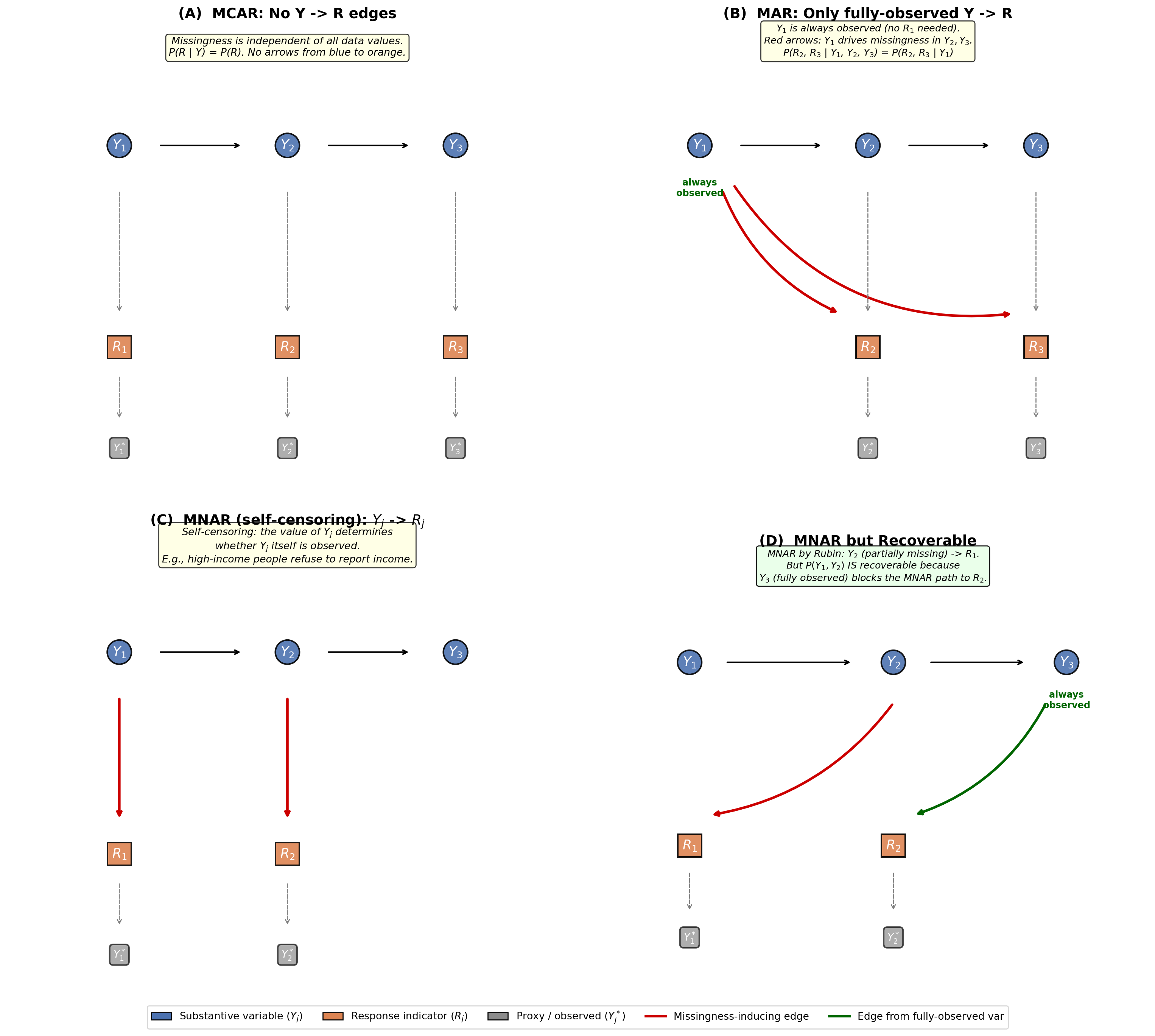
Missingness directed acyclic graphs (m-graphs) for MCAR, MAR, MNAR, and a recoverable MNAR case
Clarification on notation. Throughout these m-graphs, \(Y_1, Y_2, Y_3\) represent different variables measured on the same unit at the same time-not the same variable measured at different time points. Think of a single survey respondent providing (or failing to provide) answers to different questions. The arrows between \(Y_1 \to Y_2 \to Y_3\) represent structural or statistical relationships among variables (e.g., education predicts income, income predicts wealth), not temporal ordering. Time is not required to understand missingness mechanisms, though longitudinal settings introduce additional structure (monotone dropout) that we address separately in later sections.
Panel (A) - MCAR. There are no arrows from any substantive node (blue) to any response indicator (orange). The missingness process is completely disconnected from the data values. This is the only case where the observed data are a simple random subsample of the complete data. In practice, pure MCAR is rare-it corresponds to truly random events like equipment failures or lost mail.
Concrete examples:
A laboratory technician accidentally drops 15 out of 200 blood samples. Which samples are destroyed has nothing to do with the patients’ cholesterol levels, age, or any other variable. The remaining 185 samples are an unbiased subsample.
A survey platform experiences a server crash during data transmission, randomly losing 8% of completed responses. The crash is unrelated to what respondents answered.
A weather station’s sensor battery dies on random days, creating gaps in the temperature record that are unrelated to the actual temperature.
In all three cases, \(P(R_j = 0)\) is the same regardless of what \(Y_1, Y_2, Y_3\) equal. Any analysis on the observed subsample is unbiased-you just have less data.
Panel (B) - MAR. The red arrows run from \(Y_1\) (which is always observed-it has no \(R_1\) node) to \(R_2\) and \(R_3\). This is the critical structural feature of MAR: the variables that drive missingness are themselves fully observed. Because \(Y_1\) is always available, we can condition on it and “explain away” the missingness. This is why likelihood-based methods (EM, FIML) and MI work under MAR-they implicitly condition on all observed data, which by assumption captures everything that drives the missingness process.
Concrete examples:
Credit survey.\(Y_1\) = education level (always recorded from administrative data), \(Y_2\) = annual income (self-reported, sometimes missing), \(Y_3\) = net worth (self-reported, sometimes missing). People with lower education are less likely to report income and wealth-perhaps because the survey is more burdensome, or because they distrust the institution. But conditional on education level, whether someone reports income does not depend on their actual income. The red arrows run from education (\(Y_1\), always observed) to the missingness indicators \(R_2\) (income) and \(R_3\) (wealth).
Clinical trial.\(Y_1\) = baseline severity score (measured at enrollment for every patient), \(Y_2\) = six-month clinical outcome (sometimes missing due to dropout). Sicker patients at baseline drop out more often. But conditional on baseline severity, the dropout probability does not depend on what the six-month outcome would have been. The red arrow: baseline severity → \(R_2\) (dropout indicator).
Firm-level financial data.\(Y_1\) = stock exchange listing (HOSE vs. HNX, always known), \(Y_2\) = book equity (sometimes missing from filings). Firms on the smaller exchange (HNX) have weaker disclosure requirements and are more likely to have missing financials. Conditional on which exchange the firm lists on, whether book equity is reported does not depend on the book equity value itself.
The key test for MAR is: can I identify the variables that drive missingness, and are those variables fully observed? If yes, conditioning on them makes the missingness ignorable.
Panel (C) - MNAR (self-censoring). The red arrows run from \(Y_j\) to its own \(R_j\). Whether \(Y_1\) is observed depends on the value of \(Y_1\) itself. This is the classic nonignorable case. The information needed to correct for the missingness is exactly the information that is missing. Without additional assumptions (exclusion restrictions, parametric models, or sensitivity analysis), the full-data distribution is not identified.
Concrete examples:
Income nonresponse.\(Y_1\) = income. High earners are less likely to report their income on surveys-not because of their education or occupation (those are other variables), but because of the income value itself. The arrow runs from income directly to its own missingness indicator: \(Y_1 \to R_1\). You cannot condition on income to remove the bias because income is the variable that is missing.
Side-effect dropout.\(Y_2\) = severity of drug side effects at month 6. Patients who experience severe side effects drop out of the trial because the side effects are severe. The unobserved \(Y_2\) value (which would have been high) is the very reason \(Y_2\) is missing. No amount of baseline data corrects this-the arrow is \(Y_2 \to R_2\).
Corporate earnings management.\(Y_2\) = true earnings. Firms with very poor earnings are more likely to delay or omit their financial filings. The missingness in earnings is driven by the earnings value itself. Conditional on everything else you observe (size, industry, exchange), the probability of non-filing still depends on unobserved earnings.
Student course evaluations.\(Y_1\) = student satisfaction score. Highly dissatisfied students are more likely to skip the evaluation-the missing responses are systematically more negative than the observed ones. The arrow is \(Y_1 \to R_1\).
In every case, the pattern is the same: the variable’s own value drives its missingness. The observed data cannot tell you what the missing values would have been without additional structural assumptions.
Panel (D) - MNAR but recoverable (Mohan & Pearl’s key contribution). This case fails Rubin’s MAR condition: \(Y_2\), which is itself partially missing, influences \(R_1\) (the red arrow from \(Y_2\) to \(R_1\)). Under Rubin’s taxonomy, this entire system is classified as MNAR with no general recourse.
But the graphical framework reveals additional structure. Notice that \(Y_2\)’s own missingness (\(R_2\)) is driven by \(Y_3\) (always observed)-the green arrow from \(Y_3\) to \(R_2\). This means \(P(Y_2)\) can be recovered from observed data: among the units where \(Y_2\) is observed (\(R_2 = 1\)), the selection was driven only by \(Y_3\) (which we see for everyone), so we can reweight using \(P(R_2 = 1 \mid Y_3)\) to reconstruct the full distribution of \(Y_2\). Once \(P(Y_2)\) is identified, we can adjust for the MNAR path \(Y_2 \to R_1\) and recover \(P(Y_1)\) as well.
Concrete example:
\(Y_1\) = income (sometimes missing), \(Y_2\) = occupation type (sometimes missing), \(Y_3\) = education level (always observed from administrative records). The mechanism works as follows:
Green arrow (\(Y_3 \to R_2\)): Whether someone reports their occupation depends on education level. College graduates are more forthcoming in surveys. Since education is always available, we can model this and reweight to recover the full distribution of occupation.
Red arrow (\(Y_2 \to R_1\)): Whether someone reports their income depends on their occupation. Informal-sector workers are less likely to report income. This makes the system MNAR under Rubin-occupation is partially missing and yet drives income’s missingness.
But the query\(P(\text{income})\) is recoverable: First, reconstruct \(P(\text{occupation})\) by reweighting on education (green arrow path). Then, reconstruct \(P(\text{income})\) by adjusting for occupation using the now-identified \(P(\text{occupation})\).
This is the central insight of the graphical approach: recoverability depends on the topology of the m-graph, not just on Rubin’s three-category classification. Some MNAR problems have enough observed structure to identify the target query; others do not. The graphical framework provides an algorithmic test for this: you trace the paths from substantive variables to their missingness indicators and ask whether every path passes through a fully-identified node.
When is Panel (D) practically relevant?
It arises whenever the “chain” of missingness can be unwound step by step. If the variable that causes missingness elsewhere is itself missing but recoverable (because its missingness is driven by something observed), the entire system can be sequentially identified. Mohan and Pearl (2021) formalize this as a fixpoint algorithm on the m-graph: iteratively identify variables whose missingness depends only on already-identified quantities, then use those to unlock the next layer.
Demonstrate recoverability: correcting MNAR bias using m-graph structure
def demonstrate_recoverability(n=10000, n_sims=500, rng_base=42):""" Show that even under MNAR (by Rubin's definition), a graph-aware estimator can recover E[Y2] when the m-graph reveals recoverability. Setup (matching Panel D): - Y1, Y2, Y3 are jointly normal - R2 depends on Y3 (fully observed) -> Y2 is recoverable - R1 depends on Y2 (partially observed) -> system is MNAR overall Estimators: 1. Complete-case mean (biased) 2. EM under MAR (biased for E[Y1] because R1 mechanism is truly MNAR) 3. IPW using P(R2=1|Y3) - graph-identified adjustment (consistent for E[Y2] because R2 \perp Y2 | Y3) """ results = {'CC': [], 'IPW_graph': []}for sim inrange(n_sims): rng = np.random.default_rng(rng_base + sim) Sigma = np.array([ [1.0, 0.6, 0.3], [0.6, 1.0, 0.5], [0.3, 0.5, 1.0] ]) data = rng.multivariate_normal([0, 0, 0], Sigma, n) Y1, Y2, Y3 = data[:, 0], data[:, 1], data[:, 2]# R2 depends on Y3 (fully observed) - this makes E[Y2] recoverable p_R2 = expit(0.5+1.5* Y3) R2 = rng.random(n) < p_R2# 1. CC mean (biased) results['CC'].append(Y2[R2].mean())# 2. IPW using graphically identified P(R2=1 | Y3)# Fit logistic regression: R2 ~ Y3from sklearn.linear_model import LogisticRegression lr = LogisticRegression(max_iter=1000, C=1e6) lr.fit(Y3.reshape(-1, 1), R2.astype(int)) pi_hat = np.clip(lr.predict_proba(Y3.reshape(-1, 1))[:, 1], 0.02, 0.98)# Hajek estimator weights = R2.astype(float) / pi_hat ipw_mean = np.sum(weights * Y2) / np.sum(weights) results['IPW_graph'].append(ipw_mean)return resultsrecov_results = demonstrate_recoverability(n=5000, n_sims=500)fig, ax = plt.subplots(1, 1, figsize=(10, 6))labels = ['Complete cases\n(ignores m-graph)', 'IPW with P($R_2$|$Y_3$)\n(uses m-graph structure)']data_plot = [np.array(recov_results['CC']), np.array(recov_results['IPW_graph'])]bp = ax.boxplot(data_plot, labels=labels, patch_artist=True, showfliers=False, medianprops=dict(color='black'), widths=0.5)bp['boxes'][0].set_facecolor('#C44E52')bp['boxes'][0].set_alpha(0.6)bp['boxes'][1].set_facecolor('#55A868')bp['boxes'][1].set_alpha(0.6)ax.axhline(0, color='red', linestyle='--', linewidth=2, label='True E[$Y_2$] = 0')ax.set_ylabel('Estimate of E[$Y_2$]', fontsize=12)ax.set_title('Recoverability: The m-Graph Tells Us Which ''Adjustment Set Removes Bias\n''(Overall mechanism is MNAR, but E[$Y_2$] is ''recoverable via $Y_3$)', fontsize=13)ax.legend(fontsize=11)# Annotationsfor i, (name, vals) inenumerate(recov_results.items()): vals = np.array(vals) bias = np.mean(vals) rmse = np.sqrt(np.mean(vals**2)) ax.text(i +1, ax.get_ylim()[0] +0.01, f'bias = {bias:.4f}\nRMSE = {rmse:.4f}', ha='center', fontsize=11, fontweight='bold', color='darkred'ifabs(bias) >0.01else'darkgreen', bbox=dict(boxstyle='round,pad=0.2', facecolor='white', alpha=0.8))plt.tight_layout()plt.show()
C:\Users\miken\AppData\Local\Temp\ipykernel_7304\2847058945.py:61: MatplotlibDeprecationWarning:

The 'labels' parameter of boxplot() has been renamed 'tick_labels' since Matplotlib 3.9; support for the old name will be dropped in 3.11.
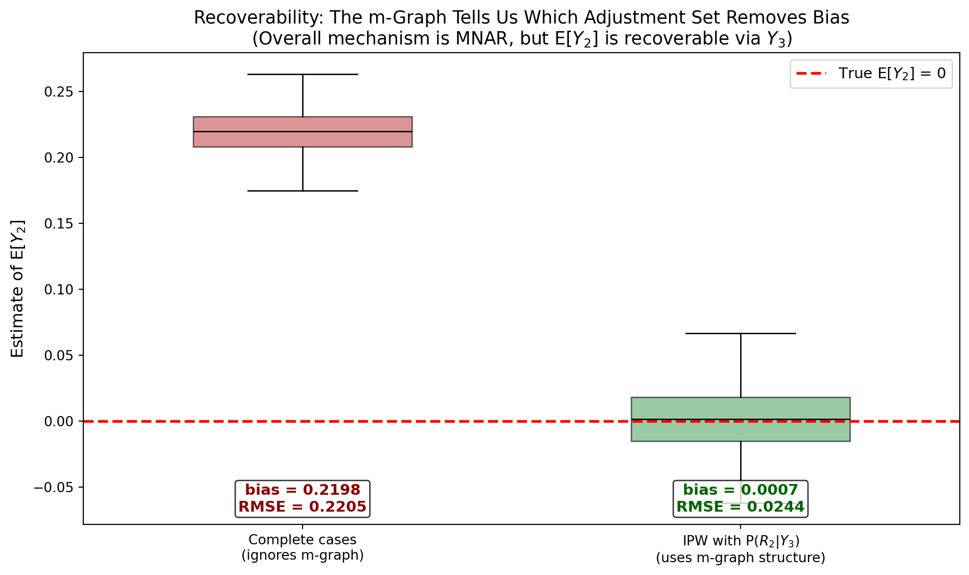
Recoverability in action: using the m-graph to correct MNAR bias through IPW on the graphically identified adjustment set
This simulation implements Panel (D) of the m-graph figure.
The overall missingness pattern is MNAR (Y2, which has missing values, causes missingness in Y1 via Y2 -> R1). Under Rubin’s framework, this entire system is classified as MNAR with no general solution.
But the m-graph reveals that for the specific query E[Y2], the missingness in Y2 is driven ONLY by Y3 (fully observed). The m-graph edge R2 <- Y3 means:
\[
P(R2 = 1 | Y1, Y2, Y3) = P(R2 = 1 | Y3)
\]
This is a local MAR condition for Y2 with respect to Y3. The IPW estimator using P(R2=1|Y3) as the propensity score is consistent:
print(f"""Results: CC bias: {np.mean(recov_results['CC']):.4f} IPW (m-graph): {np.mean(recov_results['IPW_graph']):.4f}""")
Results:
  CC bias:        0.2198
  IPW (m-graph):  0.0007
The graph-based IPW estimator eliminates the bias that CC exhibits, confirming recoverability. This works because the m-graph decomposes the global MNAR mechanism into local conditional independence statements, some of which are testable and actionable.
Practical implication: Before concluding that “the data are MNAR and nothing can be done,” draw the m-graph and check whether your specific estimand is recoverable. Mohan & Pearl (2021) provide a complete algorithm for this determination.
57.1.5 The Heckman Selection Model Perspective
In econometrics, the dominant framework for nonignorable missingness is the Heckman selection model(Heckman 1979), which predates Rubin’s taxonomy and approaches the problem from a latent variable perspective.
Setup: Consider the outcome equation and selection equation:
where \(Y_i\) is observed only if \(M_i = 0\) (i.e., \(S_i^* > 0\)). If \((\varepsilon_i, \eta_i)\) are jointly normal with correlation \(\rho\), then:
where \(\lambda(\cdot) = \phi(\cdot)/\Phi(\cdot)\) is the inverse Mills ratio (the ratio of the standard normal PDF to CDF). The term \(\rho \sigma_\varepsilon \lambda(Z_i'\gamma)\) is the selection bias correction.
Heckman’s two-step estimator:
Estimate \(\gamma\) by probit regression of \((1-M_i)\) on \(Z_i\).
Compute \(\hat{\lambda}_i = \lambda(Z_i'\hat{\gamma})\) for the observed subsample.
Regress \(Y_i\) on \((X_i, \hat{\lambda}_i)\) using OLS on the observed subsample.
The coefficient on \(\hat{\lambda}_i\) estimates \(\rho \sigma_\varepsilon\), and the coefficient on \(X_i\) estimates \(\beta\) consistently.
Identification: Heckman’s model requires an exclusion restriction: at least one variable in \(Z_i\) that is not in \(X_i\) (i.e., an instrument that affects selection but not the outcome directly). Without this, \(\beta\) is identified only through the nonlinearity of \(\lambda(\cdot)\), which is fragile.
Connection to Rubin’s taxonomy:
If \(\rho = 0\): The mechanism is MAR (missingness depends on \(Z_i\) but not on \(\varepsilon_i\), and hence not on \(Y_i\) conditional on \(X_i\)).
If \(\rho \neq 0\): The mechanism is MNAR (missingness depends on \(\eta_i\), which is correlated with \(\varepsilon_i\) and hence with \(Y_i\)).
57.2 Testing and Diagnosing Missingness Mechanisms
A fundamental limitation of missing data analysis is that the missingness mechanism is generally not testable from the observed data. This is because the mechanism describes the relationship between missingness and the missing values themselves, which are by definition unobserved. However, several diagnostic tools can provide partial evidence.
57.2.1 Little’s MCAR Test
R. J. Little (1988) proposed a multivariate test of MCAR. The test is based on the idea that under MCAR, the means of each variable should be the same across all missing data patterns.
Setup: Let \(J\) index the distinct missing data patterns observed in the data, and let \(n_j\) be the number of observations with pattern \(j\). For each pattern \(j\), let \(\bar{Y}_j^{\text{obs}}\) be the vector of means of the observed variables and let \(\hat{\mu}\) and \(\hat{\Sigma}\) be the ML estimates of the mean and covariance under a multivariate normal model. The test statistic is:
where \(\hat{\mu}_j^{\text{obs}}\) and \(\hat{\Sigma}_j^{\text{obs}}\) are the subvectors/submatrices of \(\hat{\mu}\) and \(\hat{\Sigma}\) corresponding to the observed variables in pattern \(j\). Under \(H_0: \text{MCAR}\) and multivariate normality:
where \(p_j\) is the number of observed variables in pattern \(j\).
Limitations:
Rejection implies non-MCAR but does not distinguish MAR from MNAR.
Failure to reject does not confirm MCAR (may lack power).
Assumes multivariate normality.
57.2.2 Auxiliary Variable Approaches
A practical diagnostic involves testing whether missingness in variable \(Y_j\) is associated with observed values of other variables \(Y_k\) (\(k \neq j\)):
Create the binary indicator \(M_j\) for missingness in \(Y_j\).
Test association between \(M_j\) and each observed \(Y_k\) using \(t\)-tests (continuous \(Y_k\)) or \(\chi^2\) tests (categorical \(Y_k\)).
If \(\alpha_k \neq 0\) for some \(k\), this is evidence against MCAR (consistent with MAR or MNAR). If no associations are found, this is consistent with MCAR but does not confirm it.
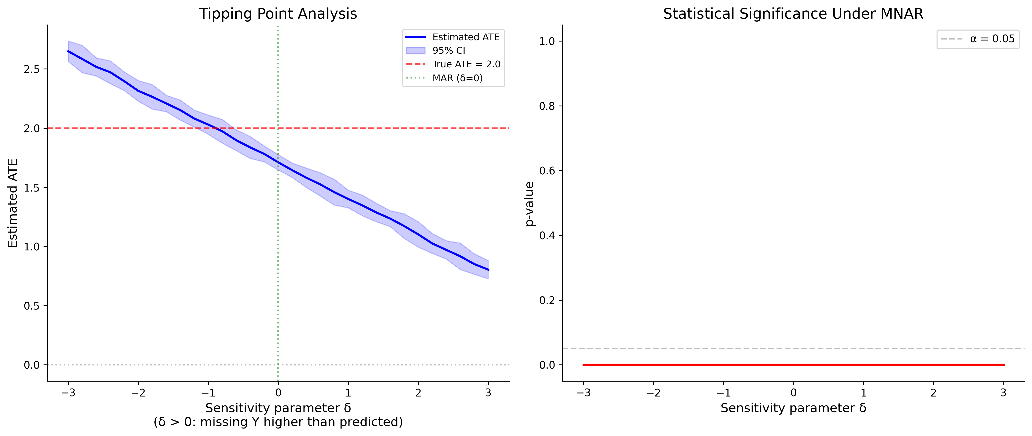
57.2.3 Sensitivity Analysis for Untestable Assumptions
Since MNAR versus MAR is generally untestable, the gold standard is sensitivity analysis: conduct the primary analysis under MAR, then examine how conclusions change under plausible MNAR departures.
We will develop formal sensitivity analysis frameworks in Section 57.12.
57.3 Setup: Simulation Infrastructure
Import libraries and configure environment
import numpy as npimport pandas as pdimport matplotlib.pyplot as pltimport seaborn as snsfrom scipy import statsfrom scipy.optimize import minimizefrom scipy.special import expit # logistic/sigmoid functionimport warningswarnings.filterwarnings('ignore')# For reproducibilityrng = np.random.default_rng(42)# Plotting configurationplt.rcParams.update({'figure.figsize': (10, 7),'font.size': 12,'axes.titlesize': 14,'axes.labelsize': 12,'xtick.labelsize': 10,'ytick.labelsize': 10,'legend.fontsize': 10,'figure.dpi': 150,'savefig.dpi': 150,'axes.spines.top': False,'axes.spines.right': False})# Color palettecolors = sns.color_palette("colorblind", 10)print("Environment configured successfully.")print(f"NumPy version: {np.__version__}")print(f"Pandas version: {pd.__version__}")
We define a suite of data generating processes (DGPs) that will be reused throughout the chapter. Each DGP produces complete data, and separate functions impose different missingness mechanisms.
Define data generating processes
def generate_linear_dgp(n=1000, p=5, beta=None, sigma=1.0, rng=None):""" Generate data from a linear model: Y = X @ beta + epsilon. Parameters ---------- n : int Sample size. p : int Number of covariates (excluding intercept). beta : array-like, optional True coefficients (length p+1, including intercept). sigma : float Error standard deviation. rng : np.random.Generator Random number generator. Returns ------- X : ndarray of shape (n, p) Covariate matrix. Y : ndarray of shape (n,) Outcome variable. beta_true : ndarray True coefficient vector. """if rng isNone: rng = np.random.default_rng()if beta isNone: beta = np.concatenate([[2.0], rng.standard_normal(p)]) X = rng.standard_normal((n, p))# Introduce correlation among covariates L = np.eye(p)for i inrange(1, p): L[i, 0] =0.3# correlation with first variable X = X @ L epsilon = rng.normal(0, sigma, n) Y = beta[0] + X @ beta[1:] + epsilonreturn X, Y, betadef generate_treatment_dgp(n=1000, tau=2.0, rng=None):""" Generate data from a treatment effects model with confounding. Y(0) = alpha + X @ gamma + epsilon Y(1) = Y(0) + tau + heterogeneity Treatment assignment depends on X (confounding). Parameters ---------- n : int Sample size. tau : float Average treatment effect. rng : np.random.Generator Random number generator. Returns ------- dict with keys: X, D, Y, Y0, Y1, tau_true """if rng isNone: rng = np.random.default_rng()# Covariates X1 = rng.standard_normal(n) X2 = rng.standard_normal(n) X = np.column_stack([X1, X2])# Potential outcomes Y0 =1.0+0.5* X1 +0.3* X2 + rng.normal(0, 1, n) Y1 = Y0 + tau +0.5* X1 # heterogeneous treatment effect# Treatment assignment (confounded) propensity = expit(0.5+0.8* X1 -0.5* X2) D = rng.binomial(1, propensity, n)# Observed outcome Y = D * Y1 + (1- D) * Y0return {'X': X, 'D': D, 'Y': Y, 'Y0': Y0, 'Y1': Y1,'tau_true': tau, 'propensity': propensity }def generate_multivariate_normal(n=1000, p=4, rho=0.5, rng=None):""" Generate data from a multivariate normal distribution. Parameters ---------- n : int Sample size. p : int Dimension. rho : float Common pairwise correlation. rng : np.random.Generator Random number generator. Returns ------- data : ndarray of shape (n, p) mu : ndarray Sigma : ndarray """if rng isNone: rng = np.random.default_rng() mu = np.arange(1, p +1, dtype=float) Sigma = np.full((p, p), rho) + np.eye(p) * (1- rho) data = rng.multivariate_normal(mu, Sigma, n)return data, mu, Sigma
57.3.2 Missingness Imposing Functions
Functions to impose different missingness mechanisms
def impose_mcar(data, prob_missing=0.3, columns=None, rng=None):""" Impose MCAR missingness. Each value in specified columns is independently missing with probability prob_missing. """if rng isNone: rng = np.random.default_rng() df = pd.DataFrame(data.copy())if columns isNone: columns = df.columnsfor col in columns: mask = rng.random(len(df)) < prob_missing df.loc[mask, col] = np.nanreturn dfdef impose_mar(data, dep_col=0, miss_col=1, beta_mar=2.0, base_prob=0.3, rng=None):""" Impose MAR missingness on miss_col depending on dep_col. P(M_{miss_col} = 1 | data) = expit(beta_0 + beta_mar * data[:, dep_col]) where beta_0 is calibrated so that marginal P(missing) ≈ base_prob. Parameters ---------- data : ndarray Complete data matrix. dep_col : int Column index that drives missingness (always observed). miss_col : int Column index where missingness is imposed. beta_mar : float Strength of MAR dependence. base_prob : float Target marginal probability of missingness. rng : np.random.Generator Returns ------- df : DataFrame with NaN imposed on miss_col. true_probs : array of true missingness probabilities. """if rng isNone: rng = np.random.default_rng() df = pd.DataFrame(data.copy())# Calibrate intercept to achieve target marginal missing rate x = data[:, dep_col]# Use bisection to find beta_0def obj(beta_0): probs = expit(beta_0 + beta_mar * x)return np.mean(probs) - base_probfrom scipy.optimize import brentqtry: beta_0 = brentq(obj, -10, 10)exceptValueError: beta_0 = np.log(base_prob / (1- base_prob)) true_probs = expit(beta_0 + beta_mar * x) mask = rng.random(len(df)) < true_probs df.iloc[mask, miss_col] = np.nanreturn df, true_probsdef impose_mnar(data, miss_col=0, beta_mnar=2.0, base_prob=0.3, rng=None):""" Impose MNAR missingness: missingness in miss_col depends on the value of miss_col itself. P(M = 1) = expit(beta_0 + beta_mnar * data[:, miss_col]) """if rng isNone: rng = np.random.default_rng() df = pd.DataFrame(data.copy()) y = data[:, miss_col]from scipy.optimize import brentqdef obj(beta_0): probs = expit(beta_0 + beta_mnar * y)return np.mean(probs) - base_probtry: beta_0 = brentq(obj, -10, 10)exceptValueError: beta_0 = np.log(base_prob / (1- base_prob)) true_probs = expit(beta_0 + beta_mnar * y) mask = rng.random(len(df)) < true_probs df.iloc[mask, miss_col] = np.nanreturn df, true_probsdef impose_mixed_missingness(data, rng=None):""" Impose a realistic pattern: - Column 0: MCAR (prob=0.1) - Column 1: MAR depending on Column 0 - Column 2: MNAR depending on own value """if rng isNone: rng = np.random.default_rng() df = pd.DataFrame(data.copy()) n =len(df)# MCAR on column 0 mask0 = rng.random(n) <0.1 df.iloc[mask0, 0] = np.nan# MAR on column 1 (depends on column 0, using original data) prob1 = expit(-0.5+1.5* data[:, 0]) mask1 = rng.random(n) < prob1 df.iloc[mask1, 1] = np.nan# MNAR on column 2 prob2 = expit(-1.0+1.0* data[:, 2]) mask2 = rng.random(n) < prob2 df.iloc[mask2, 2] = np.nanreturn df
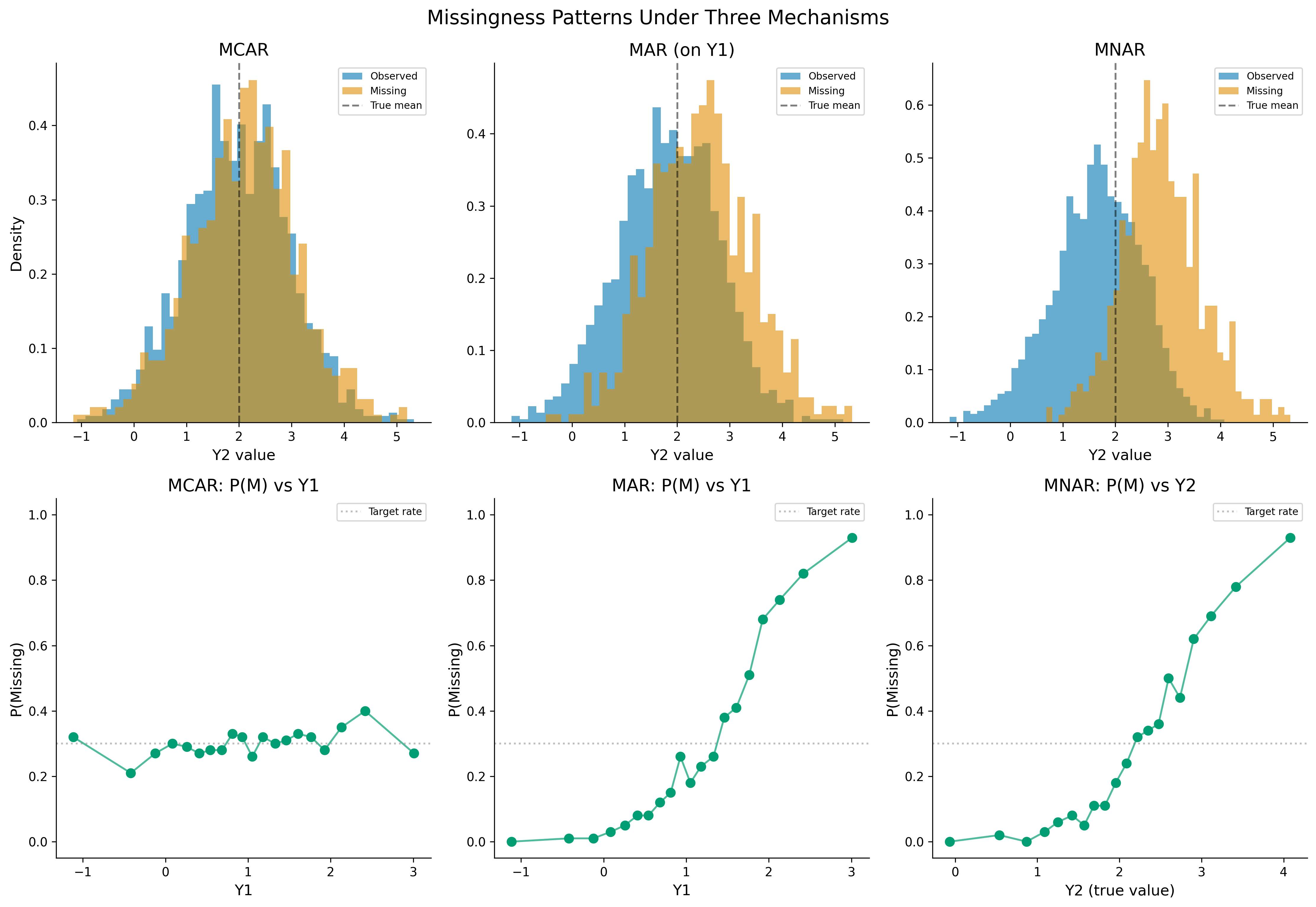
57.4 Visualizing Missingness Patterns
Before applying any method, it is essential to understand the structure and extent of missingness in the data. This section provides diagnostic visualizations.
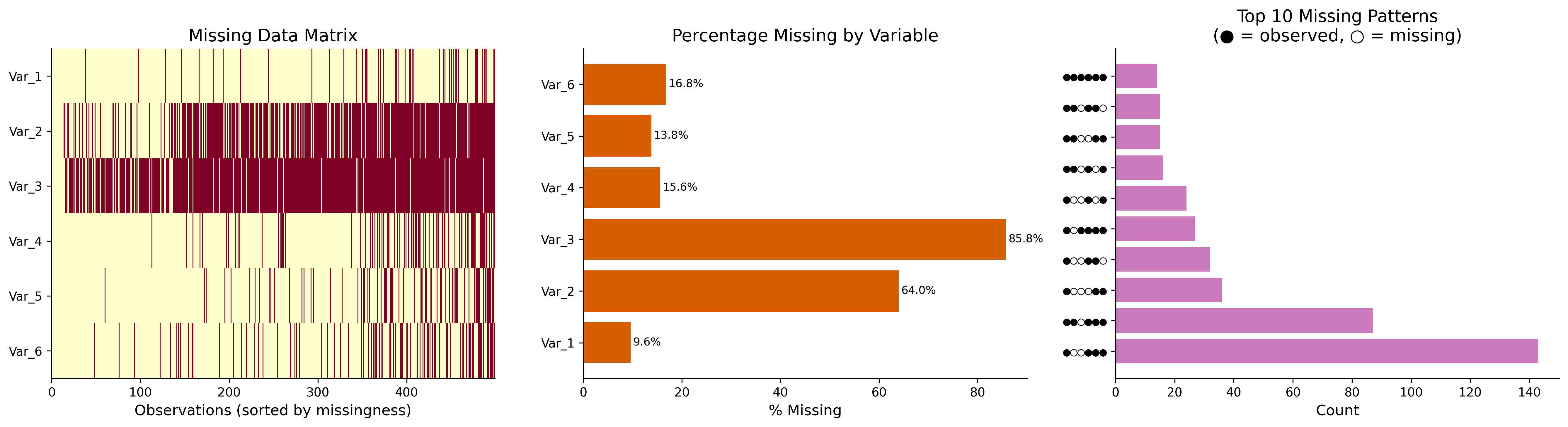
Visualize missingness patterns for the three mechanisms
# Generate data with mixed missingness across multiple columnsdata_mixed, _, _ = generate_multivariate_normal(n=500, p=6, rho=0.4, rng=rng)df_mixed = impose_mixed_missingness(data_mixed, rng=rng)# Add some MCAR on columns 3, 4, 5for c in [3, 4, 5]: mask_c = rng.random(500) <0.15 df_mixed.iloc[mask_c, c] = np.nandf_mixed.columns = [f'Var_{i+1}'for i inrange(6)]fig, axes = plt.subplots(1, 3, figsize=(18, 5))# Panel 1: Missing data matrix (sorted by total missingness per row)miss_matrix = df_mixed.isnull().astype(int)row_sums = miss_matrix.sum(axis=1)sorted_idx = row_sums.sort_values().indexax = axes[0]ax.imshow(miss_matrix.loc[sorted_idx].values.T, aspect='auto', cmap='YlOrRd', interpolation='none')ax.set_yticks(range(6))ax.set_yticklabels(df_mixed.columns)ax.set_xlabel('Observations (sorted by missingness)')ax.set_title('Missing Data Matrix')# Panel 2: Percentage missing per variableax = axes[1]pct_missing = df_mixed.isnull().mean() *100bars = ax.barh(range(6), pct_missing, color=colors[3])ax.set_yticks(range(6))ax.set_yticklabels(df_mixed.columns)ax.set_xlabel('% Missing')ax.set_title('Percentage Missing by Variable')for bar, pct inzip(bars, pct_missing): ax.text(bar.get_width() +0.5, bar.get_y() + bar.get_height()/2,f'{pct:.1f}%', va='center', fontsize=9)# Panel 3: Missing data patternsax = axes[2]patterns = miss_matrix.apply(lambda row: ''.join(row.astype(str)), axis=1)pattern_counts = patterns.value_counts().head(10)y_pos =range(len(pattern_counts))ax.barh(y_pos, pattern_counts.values, color=colors[4])ax.set_yticks(y_pos)ax.set_yticklabels([f"{''.join(['●'if c=='0'else'○'for c in p])}"for p in pattern_counts.index], fontfamily='monospace')ax.set_xlabel('Count')ax.set_title('Top 10 Missing Patterns\n(● = observed, ○ = missing)')plt.tight_layout()plt.show()
Missingness pattern matrix showing co-occurrence of missing values
57.4.1 Little’s MCAR Test Implementation
Implementation of Little’s MCAR test
def littles_mcar_test(data):""" Perform Little's (1988) MCAR test. Parameters ---------- data : DataFrame Data with missing values (NaN). Returns ------- dict with 'statistic', 'df', 'p_value' Notes ----- Assumes multivariate normality. Uses EM estimates for the mean and covariance. """ df = data.copy() n, p = df.shape# Estimate mean and covariance using available cases (simplified EM)# Use pairwise complete observations mu_hat = df.mean().values sigma_hat = df.cov().values# Handle any NaN in sigma_hat with simple imputation for estimationfor i inrange(p):for j inrange(p):if np.isnan(sigma_hat[i, j]): sigma_hat[i, j] =0.0if i != j else1.0# Identify missing data patterns miss_patterns = df.isnull() pattern_strings = miss_patterns.apply(lambda row: tuple(row.values), axis=1 ) unique_patterns = pattern_strings.unique() d2 =0.0 df_total =0for pattern in unique_patterns:ifall(not v for v in pattern):continue# Complete cases, skipifall(v for v in pattern):continue# All missing, skip# Indices of rows with this pattern mask = pattern_strings == pattern n_j = mask.sum()if n_j <2:continue# Observed variable indices for this pattern obs_vars = [i for i, v inenumerate(pattern) ifnot v]iflen(obs_vars) ==0:continue# Subsample means of observed variables y_bar_j = df.loc[mask, df.columns[obs_vars]].mean().values# Expected means and covariance (from full-data estimates) mu_j = mu_hat[obs_vars] sigma_j = sigma_hat[np.ix_(obs_vars, obs_vars)]# Contribution to test statistictry: sigma_j_inv = np.linalg.inv(sigma_j) diff = y_bar_j - mu_j d2 += n_j * diff @ sigma_j_inv @ diff df_total +=len(obs_vars)except np.linalg.LinAlgError:continue df_stat = df_total - pif df_stat <=0:return {'statistic': np.nan, 'df': df_stat, 'p_value': np.nan, 'conclusion': 'Insufficient patterns'} p_value =1- stats.chi2.cdf(d2, df_stat) conclusion = ("Reject MCAR (p < 0.05)"if p_value <0.05else"Fail to reject MCAR (p >= 0.05)" )return {'statistic': d2, 'df': df_stat, 'p_value': p_value, 'conclusion': conclusion }# Apply to our three datasetsprint("="*60)print("Little's MCAR Test Results")print("="*60)for name, df_test in [('MCAR', data_mcar), ('MAR', data_mar), ('MNAR', data_mnar)]: df_test.columns = col_names result = littles_mcar_test(df_test)print(f"\n{name}:")print(f" Test statistic: {result['statistic']:.3f}")print(f" Degrees of freedom: {result['df']}")print(f" p-value: {result['p_value']:.6f}")print(f" Conclusion: {result['conclusion']}")
============================================================
Little's MCAR Test Results
============================================================

MCAR:
  Test statistic: nan
  Degrees of freedom: -1
  p-value: nan
  Conclusion: Insufficient patterns

MAR:
  Test statistic: nan
  Degrees of freedom: -1
  p-value: nan
  Conclusion: Insufficient patterns

MNAR:
  Test statistic: nan
  Degrees of freedom: -1
  p-value: nan
  Conclusion: Insufficient patterns
57.5 Traditional Methods and Their Properties
We now systematically examine the most commonly used methods for handling missing data, deriving their statistical properties under each missingness mechanism.
57.5.1 Listwise Deletion (Complete-Case Analysis)
Method: Discard all observations with any missing values and analyze the remaining complete cases.
Statistical properties:
Mechanism
Unbiased?
Consistent?
Efficient?
MCAR
Yes
Yes
No (loses data)
MAR
Generally No
Generally No
No
MNAR
No
No
No
When listwise deletion works under MAR:
R. J. Little and Rubin (2019) show that complete-case analysis can yield valid estimates of regression coefficients even under MAR in specific settings. If \(Y\) is the outcome, \(X\) is a covariate vector, and missingness depends only on \(X\) (all of which are observed in complete cases), then the complete-case regression of \(Y\) on \(X\) is consistent. This is because the complete-case analysis conditions on a function of \(X\), which is a valid conditioning set.
Formal result (White and Carlin (2010)): Consider the regression model \(E[Y \mid X] = X'\beta\). If missingness in \(Y\) depends only on \(X\) (i.e., \(P(M_Y = 1 \mid Y, X) = P(M_Y = 1 \mid X)\)), and \(X\) is fully observed, then the complete-case OLS estimator \(\hat{\beta}_{\text{cc}}\) is consistent for \(\beta\).
The Complete-Case Estimator
The formula begins with the standard Ordinary Least Squares (OLS) estimator, but restricted only to the subset of data where we have complete observations.
\(X_i\) is a column vector of features for observation \(i\).
\(X_i'\) is its transpose, making \(X_i X_i'\) a matrix.
\(Y_i\) is the scalar target variable.
\(M_i = 0\) indicates the data is observed (not missing).
Taking the Probability Limit (plim)
We want to know what happens to this estimator as our sample size \(N\) approaches infinity. To find the probability limit (\(\text{plim}\)), we multiply both the inverted term and the second term by \(1/N_{\text{cc}}\), where \(N_{\text{cc}}\) is the number of complete cases.
By the Weak Law of Large Numbers, sample averages converge in probability to their true population expectations (denoted by \(E\)).
This equation states that in a massive dataset, our complete-case calculation equals the population expectation of \(X X'\) inverted, multiplied by the population expectation of \(X Y\), strictly evaluated within the sub-population where \(M=0\).
The Missing at Random (MAR) Assumption
The fundamental assumption of the linear regression model is that the conditional expectation of \(Y\) given \(X\) is a linear function of \(X\): \[
E[Y \mid X] = X'\beta
\]
The MAR assumption states that the missingness mechanism \(M\) depends only on the observed variables \(X\), and not on the unobserved values of \(Y\). In probability terms, \(M\) and \(Y\) are conditionally independent given \(X\), written as \(M \perp Y \mid X\).
Because of this conditional independence, adding the condition \(M=0\) does not change our expectation of \(Y\) as long as we already know \(X\). Therefore: \[
E[Y \mid X, M=0] = E[Y \mid X] = X'\beta
\]
Applying the Law of Iterated Expectations (LIE)
To solve the right side of our \(\text{plim}\) equation, we need to evaluate \(E[XY \mid M=0]\). We do this using the Law of Iterated Expectations, which allows us to break a complex expectation into an inner and outer expectation.
Step 4a: Set up the LIE We condition on \(X\) inside the expectation: \[
E[XY \mid M=0] = E_{X}\left[ E_{Y}[XY \mid X, M=0] \mid M=0 \right]
\]
Step 4b: Pull out the known constant In the inner expectation \(E_{Y}[XY \mid X, M=0]\), the variable \(X\) is given as a condition. Because \(X\) is treated as a known constant inside this inner bracket, we can factor it out: \[
E[XY \mid M=0] = E_{X}\left[ X \cdot E_{Y}[Y \mid X, M=0] \mid M=0 \right]
\]
Step 4c: Substitute the true model Substitute the result from Step 3 (\(E[Y \mid X, M=0] = X'\beta\)) into the inner expectation: \[
E[XY \mid M=0] = E_{X}\left[ X (X'\beta) \mid M=0 \right]
\]
Step 4d: Pull out the\(\beta\) parameter Because \(\beta\) is a vector of constants representing the true population parameters, it can be factored out of the outer expectation entirely: \[
E[XY \mid M=0] = E[X X' \mid M=0] \beta
\]
Final Substitution and Cancellation
Now, we substitute the result from Step 4d back into the original \(\text{plim}\) equation from Step 2:
Notice that we have a matrix \(\left(E[X X' \mid M=0]\right)\) and its inverse \(\left(E[X X' \mid M=0]\right)^{-1}\) multiplied together. Any non-singular matrix multiplied by its own inverse results in the Identity Matrix (\(I\)).
\[
\text{plim} \, \hat{\beta}_{\text{cc}} = I \cdot \beta
\]
The proof demonstrates that under the strict MAR assumption on \(X\), filtering out the missing data will not bias the final coefficients. The estimator converges to the true population parameter \(\beta\).
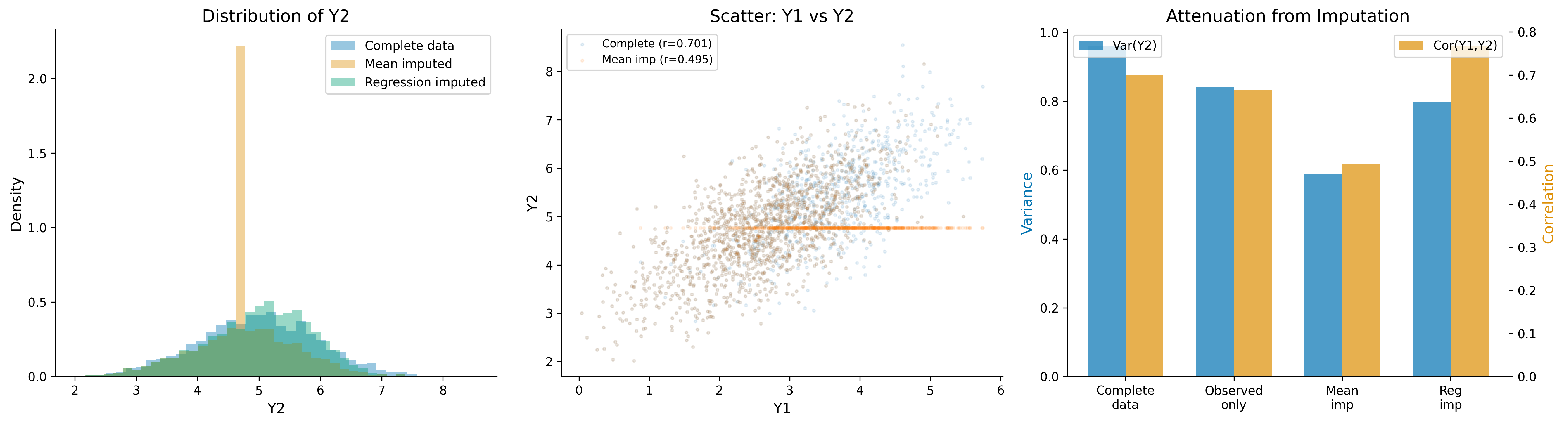
57.5.2 Mean/Mode Imputation
Method: Replace each missing value with the mean (continuous) or mode (categorical) of the observed values of that variable.
Stochastic regression imputation preserves the marginal variance but still treats imputed values as known data in subsequent analyses, leading to underestimated standard errors. Only multiple imputation properly accounts for imputation uncertainty.
57.5.4 Last Observation Carried Forward (LOCF) and Related Methods
In longitudinal data, LOCF replaces a missing value with the last observed value for that unit. While common in clinical trials (historically endorsed by FDA guidelines), it has been widely criticized:
Assumes the outcome remains constant after dropout, which is often biologically implausible.
Under MAR with a monotone dropout pattern, LOCF is generally biased.
Mallinckrod et al. (2008) and Council, National Statistics, and Handling Missing Data in Clinical Trials (2011) (the National Research Council panel) recommend against LOCF in favor of principled methods.
Baseline Observation Carried Forward (BOCF) and Worst Observation Carried Forward (WOCF) are variants used for sensitivity analysis in clinical trials but should not be primary analysis methods.
57.6 Maximum Likelihood Methods
57.6.1 The EM Algorithm
The Expectation-Maximization (EM) algorithm(Dempster, Laird, and Rubin 1977) is a general iterative procedure for ML estimation with incomplete data. It exploits the relationship between the complete-data likelihood \(L_c(\theta \mid Y_{\text{com}})\) and the observed-data likelihood \(L(\theta \mid Y_{\text{obs}})\).
General EM iteration:
Given current parameter estimates \(\theta^{(t)}\):
E-step: Compute the expected complete-data log-likelihood, where the expectation is over \(Y_{\text{mis}}\) conditional on \(Y_{\text{obs}}\) and \(\theta^{(t)}\):
where \(H(\theta \mid \theta^{(t)}) = E[\log f(Y_{\text{mis}} \mid Y_{\text{obs}}, \theta) \mid Y_{\text{obs}}, \theta^{(t)}]\), and \(H(\theta \mid \theta^{(t)}) \leq H(\theta^{(t)} \mid \theta^{(t)})\) by Jensen’s inequality.
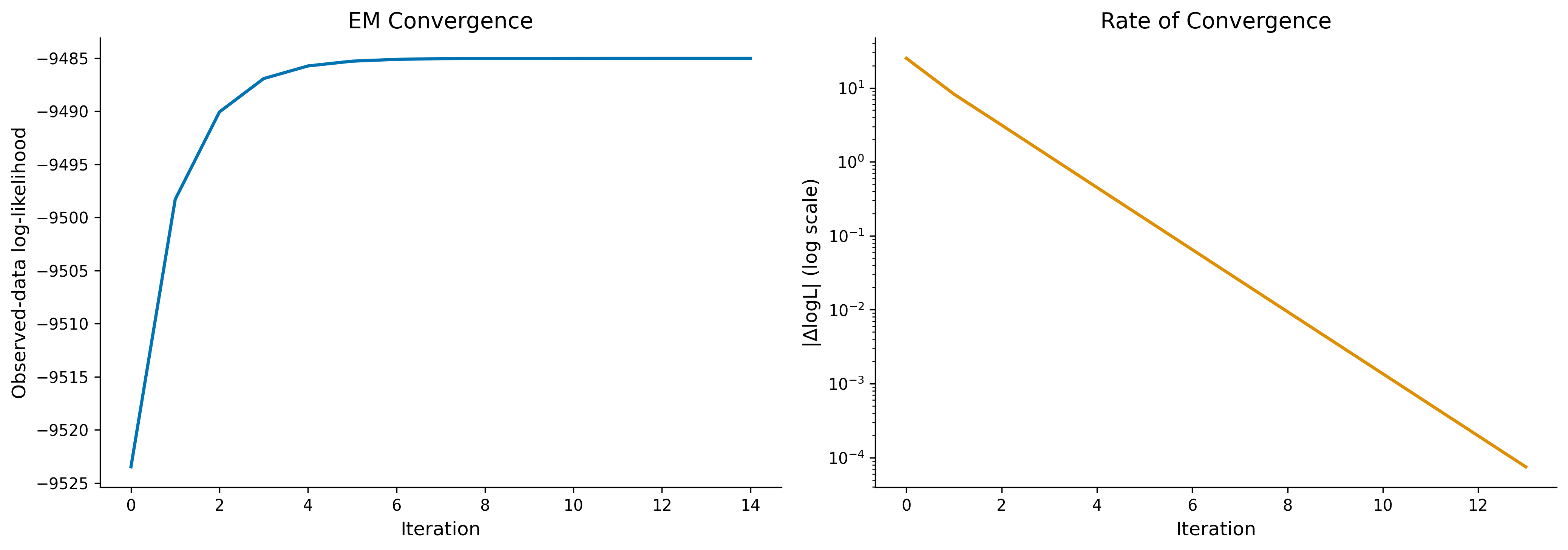
Convergence: Under regularity conditions, the sequence \(\{\theta^{(t)}\}\) converges to a stationary point of \(L(\theta \mid Y_{\text{obs}})\) (typically a local maximum).
Rate of convergence: The rate is governed by the fraction of missing information. If \(I_{\text{obs}}\) and \(I_{\text{com}}\) denote the observed and complete-data information matrices, the rate matrix is \(I_{\text{mis}} I_{\text{com}}^{-1}\), where \(I_{\text{mis}} = I_{\text{com}} - I_{\text{obs}}\).
57.6.2 EM for the Multivariate Normal
For \(Y \sim N_p(\mu, \Sigma)\) with missing data, the complete-data sufficient statistics are \(T_1 = \sum_i Y_i\) and \(T_2 = \sum_i Y_i Y_i'\).
E-step: For each observation \(i\) with missing components, compute:
EM algorithm convergence: observed-data log-likelihood
57.6.3 Full Information Maximum Likelihood (FIML)
Full Information Maximum Likelihood (FIML), also called direct maximum likelihood or raw ML, maximizes the observed-data log-likelihood directly without iterating between E and M steps. For each observation \(i\), the log-likelihood contribution uses only the observed variables for that observation:
where \(p_i\) is the number of observed variables for unit \(i\), \(\mu_i^{\text{obs}}\) and \(\Sigma_i^{\text{obs}}\) are the corresponding subvector and submatrix of \(\mu\) and \(\Sigma\).
FIML is asymptotically equivalent to EM for the same model but avoids the iterative E-step. It is particularly popular in structural equation modeling (SEM), where it is the default missing data method in software such as lavaan, Mplus, and OpenMx.
Advantages over EM: Direct access to the Hessian (observed information matrix) for standard errors; no convergence issues from EM’s iterative nature; can be combined with any optimization algorithm.
Both EM and FIML produce consistent, asymptotically efficient estimates under MAR (assuming correct model specification and parameter distinctness).
FIML for multivariate normal
def fiml_mvn(data, verbose=False):""" Full Information Maximum Likelihood for multivariate normal. Directly maximizes the observed-data log-likelihood using numerical optimization. """ifisinstance(data, pd.DataFrame): X = data.values.copy()else: X = data.copy() n, p = X.shape# Precompute observation patterns obs_patterns = []for i inrange(n): obs_idx = np.where(~np.isnan(X[i]))[0] obs_patterns.append((obs_idx, X[i, obs_idx]))def neg_loglik(params): mu = params[:p]# Reconstruct Sigma from Cholesky factor (ensures PD) L = np.zeros((p, p)) idx =0for i inrange(p):for j inrange(i +1): L[i, j] = params[p + idx] idx +=1# Ensure positive diagonalfor i inrange(p): L[i, i] = np.exp(L[i, i]) Sigma = L @ L.T loglik =0.0for obs_idx, y_obs in obs_patterns:iflen(obs_idx) ==0:continue mu_o = mu[obs_idx] Sigma_o = Sigma[np.ix_(obs_idx, obs_idx)]try: diff = y_obs - mu_o L_o = np.linalg.cholesky(Sigma_o) logdet =2* np.sum(np.log(np.diag(L_o))) solve = np.linalg.solve(L_o, diff) loglik +=-0.5* (len(obs_idx) * np.log(2*np.pi) + logdet + np.dot(solve, solve))except np.linalg.LinAlgError:return1e10return-loglik# Initialize mu_init = np.nanmean(X, axis=0) Sigma_init = np.eye(p)for i inrange(p):for j inrange(p): mask =~np.isnan(X[:, i]) &~np.isnan(X[:, j])if mask.sum() >1: Sigma_init[i, j] = np.cov(X[mask, i], X[mask, j])[0, 1] eigvals = np.linalg.eigvalsh(Sigma_init)if eigvals.min() <1e-6: Sigma_init += np.eye(p) * (1e-6- eigvals.min()) L_init = np.linalg.cholesky(Sigma_init)# Log-transform diagonal L_params = []for i inrange(p):for j inrange(i +1):if i == j: L_params.append(np.log(L_init[i, j]))else: L_params.append(L_init[i, j]) params_init = np.concatenate([mu_init, L_params]) result = minimize(neg_loglik, params_init, method='L-BFGS-B', options={'maxiter': 1000, 'ftol': 1e-12})# Extract results mu_hat = result.x[:p] L_hat = np.zeros((p, p)) idx =0for i inrange(p):for j inrange(i +1): L_hat[i, j] = result.x[p + idx] idx +=1for i inrange(p): L_hat[i, i] = np.exp(L_hat[i, i]) Sigma_hat = L_hat @ L_hat.Treturn {'mu': mu_hat,'Sigma': Sigma_hat,'loglik': -result.fun,'converged': result.success,'message': result.message }# Compare EM and FIMLfiml_result = fiml_mvn(data_mar)print("="*60)print("Comparison: EM vs FIML (MAR data)")print("="*60)print(f"\n{'':15s}{'True':>10s}{'EM':>10s}{'FIML':>10s}")print("-"*50)for j inrange(4):print(f" mu[{j}] {mu_true[j]:10.4f} "f"{em_result['mu'][j]:10.4f}{fiml_result['mu'][j]:10.4f}")print(f"\n Max |diff| in mu: "f"{np.max(np.abs(em_result['mu'] - fiml_result['mu'])):.6f}")print(f" Max |diff| in Sigma: "f"{np.max(np.abs(em_result['Sigma'] - fiml_result['Sigma'])):.6f}")
============================================================
Comparison: EM vs FIML (MAR data)
============================================================

                      True         EM       FIML
--------------------------------------------------
  mu[0]            1.0000     0.9961     0.9961
  mu[1]            2.0000     2.0144     2.0145
  mu[2]            3.0000     3.0018     3.0018
  mu[3]            4.0000     3.9702     3.9702

  Max |diff| in mu: 0.000103
  Max |diff| in Sigma: 0.000128
57.7 Multiple Imputation
57.7.1 Theory and Foundations
Multiple Imputation (MI), proposed by D. Rubin (1987), is perhaps the most widely used principled approach to missing data. The key insight is that a single imputed dataset understates uncertainty because it treats imputed values as known. MI addresses this by creating \(m\) plausible completed datasets, analyzing each, and combining results using rules that account for both within-imputation and between-imputation variability.
The three steps of MI:
Imputation: Generate \(m\) completed datasets \(\{D^{(1)}, D^{(2)}, \ldots, D^{(m)}\}\) by drawing from the posterior predictive distribution of \(Y_{\text{mis}} \mid Y_{\text{obs}}\).
Analysis: Apply the substantive analysis (e.g., regression, test) to each completed dataset, obtaining estimates \(\hat{\theta}^{(j)}\) and variance estimates \(\hat{W}^{(j)}\) for \(j = 1, \ldots, m\).
Pooling (Rubin’s rules): Combine the \(m\) results:
Point estimate:\[
\bar{\theta} = \frac{1}{m} \sum_{j=1}^m \hat{\theta}^{(j)}
\tag{57.7}\]
Total variance:\[
T = \bar{W} + \left(1 + \frac{1}{m}\right) B
\tag{57.10}\]
The factor \((1 + 1/m)\) adjusts for the finite number of imputations. As \(m \to \infty\), \(T \to \bar{W} + B\), which is the correct posterior variance of \(\theta\) under proper imputation.
Degrees of freedom for inference:
For scalar \(\theta\), the reference distribution is:
This estimates the fraction of information about \(\theta\) that is lost due to missingness. Note that this is not the same as the fraction of data that is missing-it depends on the relationship between the missingness pattern and the quantity of interest.
57.7.2 How Many Imputations?
D. Rubin (1987) originally suggested \(m = 3\) to \(5\) imputations would suffice for most purposes. More recent work has shown this can be inadequate:
White, Royston, and Wood (2011) recommend \(m \geq 100 \hat{\gamma}\), where \(\hat{\gamma}\) is the fraction of missing information (not the fraction of missing data).
Bodner (2008) recommends \(m\) at least equal to the percentage of incomplete cases.
Graham, Olchowski, and Gilreath (2007) showed that \(m = 20\) is adequate for most problems with up to 30% missing data, but more are needed with higher missing fractions or when interval estimates (confidence intervals, p-values) are important.
The cost of additional imputations is minimal compared to the cost of developing the analysis, so erring on the side of more imputations is generally advisable.
57.7.3 Multivariate Imputation by Chained Equations (MICE)
The most flexible and widely used MI procedure is MICE(Van Buuren and Groothuis-Oudshoorn 2011), also known as fully conditional specification (FCS) or sequential regression multivariate imputation (SRMI).
Algorithm:
Initialize missing values (e.g., by random draws from observed values).
For iteration \(t = 1, 2, \ldots, T\):
For each variable \(j = 1, \ldots, p\) with missing values:
Define \(Y_{-j}\) as all variables except \(j\) (using current imputed values for variables already updated in this iteration, and previous iteration’s values for those not yet updated).
Fit a model \(f(Y_j \mid Y_{-j}; \phi_j)\) using only the rows where \(Y_j\) is observed.
After \(T\) burn-in iterations, the final imputed dataset is one draw.
Repeat steps 1-3 independently \(m\) times to get \(m\) imputed datasets.
Theoretical justification:
MICE does not target a well-defined joint distribution in general. The conditional models \(f(Y_j \mid Y_{-j})\) for different \(j\) may be incompatible-there may not exist a joint distribution whose conditionals match all the specified models. Despite this, Buuren et al. (2006) and Hughes et al. (2014) showed that MICE performs well in practice, and Liu et al. (2014) proved convergence of MICE to a stationary distribution under certain conditions.
Choice of conditional models:
Variable type
Recommended model
Continuous
Linear regression (predictive mean matching)
Binary
Logistic regression
Ordinal
Ordinal logistic regression
Nominal
Multinomial logistic regression
Count
Poisson or negative binomial regression
Semi-continuous (zero-inflated)
Two-part model
Predictive Mean Matching (PMM):
PMM is the preferred method for continuous variables because it ensures imputed values are plausible (drawn from the set of observed values) and handles departures from normality. The algorithm:
Fit linear regression on observed data; draw \(\beta^*\) from posterior.
Compute predicted values \(\hat{y}_i = X_i' \beta^*\) for all cases.
For each missing \(y_i\): find the \(k\) observed cases with predicted values closest to \(\hat{y}_i\) (the “donor pool”).
Randomly select one donor and use its observed\(y\) value as the imputed value.
PMM has the attractive property that imputed values are always within the range of observed data and preserve the empirical distribution.
MICE implementation from scratch
class MICE:""" Multivariate Imputation by Chained Equations. Implements MICE with: - Linear regression for continuous variables - Predictive mean matching (PMM) - Bayesian posterior draws for proper imputation Parameters ---------- n_imputations : int Number of multiply imputed datasets. n_iterations : int Number of MICE iterations (burn-in + sampling). method : str 'normal' for Bayesian linear regression, 'pmm' for predictive mean matching. pmm_k : int Number of donors for PMM. random_state : int Random seed. """def__init__(self, n_imputations=20, n_iterations=10, method='pmm', pmm_k=5, random_state=42):self.n_imputations = n_imputationsself.n_iterations = n_iterationsself.method = methodself.pmm_k = pmm_kself.rng = np.random.default_rng(random_state)def _bayesian_regression_draw(self, X, y):""" Draw regression parameters from the posterior. Under a noninformative prior (Jeffreys), the posterior is: beta | sigma^2, data ~ N(beta_hat, sigma^2 (X'X)^{-1}) sigma^2 | data ~ InvGamma((n-p)/2, RSS/2) We draw sigma^2 first, then beta | sigma^2. """ n, p = X.shape# Add intercept X_int = np.column_stack([np.ones(n), X]) p_full = X_int.shape[1]# OLStry: XtX_inv = np.linalg.inv(X_int.T @ X_int)except np.linalg.LinAlgError: XtX_inv = np.linalg.pinv(X_int.T @ X_int) beta_hat = XtX_inv @ X_int.T @ y residuals = y - X_int @ beta_hat rss = np.sum(residuals**2) df =max(n - p_full, 1)# Draw sigma^2 from scaled inverse chi-squared sigma2_draw = rss /self.rng.chisquare(df)# Draw beta from conditional posterior beta_cov = sigma2_draw * XtX_inv# Ensure PD eigvals = np.linalg.eigvalsh(beta_cov)if eigvals.min() <0: beta_cov += np.eye(p_full) * (1e-8- eigvals.min())try: beta_draw =self.rng.multivariate_normal(beta_hat, beta_cov)except np.linalg.LinAlgError: beta_draw = beta_hat # Fallbackreturn beta_draw, np.sqrt(sigma2_draw)def _impute_column(self, data, col_idx, miss_mask):"""Impute a single column using other columns as predictors.""" other_cols = [c for c inrange(data.shape[1]) if c != col_idx]# Observed rows for this column obs_rows =~miss_mask[:, col_idx]if obs_rows.sum() <3:# Too few observations; use marginal mean data[miss_mask[:, col_idx], col_idx] = np.nanmean( data[obs_rows, col_idx])return data X_obs = data[obs_rows][:, other_cols] y_obs = data[obs_rows, col_idx] X_mis = data[miss_mask[:, col_idx]][:, other_cols]if X_mis.shape[0] ==0:return data# Draw parameters from posterior beta_draw, sigma_draw =self._bayesian_regression_draw(X_obs, y_obs) X_mis_int = np.column_stack([np.ones(X_mis.shape[0]), X_mis]) X_obs_int = np.column_stack([np.ones(X_obs.shape[0]), X_obs])ifself.method =='pmm':# Predictive mean matching pred_obs = X_obs_int @ beta_draw pred_mis = X_mis_int @ beta_drawfor i, pm inenumerate(pred_mis):# Find k closest observed predictions distances = np.abs(pred_obs - pm) donor_idx = np.argsort(distances)[:self.pmm_k] chosen =self.rng.choice(donor_idx) data[np.where(miss_mask[:, col_idx])[0][i], col_idx] =\ y_obs[chosen]else:# Normal draw pred_mis = X_mis_int @ beta_draw noise =self.rng.normal(0, sigma_draw, X_mis.shape[0]) data[miss_mask[:, col_idx], col_idx] = pred_mis + noisereturn datadef fit_transform(self, data):""" Generate m multiply imputed datasets. Parameters ---------- data : DataFrame or ndarray Data with NaN for missing values. Returns ------- list of ndarrays: m imputed datasets """ifisinstance(data, pd.DataFrame): X_orig = data.values.copy() columns = data.columnselse: X_orig = data.copy() columns =None n, p = X_orig.shape miss_mask = np.isnan(X_orig)# Columns with missing data (in order of least to most missing) cols_with_missing = np.where(miss_mask.any(axis=0))[0] n_missing_per_col = miss_mask.sum(axis=0) cols_with_missing = cols_with_missing[ np.argsort(n_missing_per_col[cols_with_missing]) ] imputed_datasets = []for m inrange(self.n_imputations):# Initialize: random draw from observed values X_imp = X_orig.copy()for col in cols_with_missing: obs_vals = X_orig[~miss_mask[:, col], col] n_miss = miss_mask[:, col].sum() X_imp[miss_mask[:, col], col] =self.rng.choice( obs_vals, size=n_miss, replace=True )# Iteratefor t inrange(self.n_iterations):for col in cols_with_missing: X_imp =self._impute_column(X_imp, col, miss_mask)if columns isnotNone: imputed_datasets.append( pd.DataFrame(X_imp, columns=columns))else: imputed_datasets.append(X_imp)return imputed_datasetsdef rubins_rules(estimates, variances):""" Apply Rubin's combining rules to multiple imputation results. Parameters ---------- estimates : list of arrays Point estimates from each imputed dataset. variances : list of arrays Variance estimates from each imputed dataset. Returns ------- dict with 'estimate', 'within_var', 'between_var', 'total_var', 'se', 'fmi', 'df' """ m =len(estimates) estimates = np.array(estimates) variances = np.array(variances)# Point estimate theta_bar = estimates.mean(axis=0)# Within-imputation variance W_bar = variances.mean(axis=0)# Between-imputation variance B = estimates.var(axis=0, ddof=1)# Total variance T = W_bar + (1+1/m) * B# Fraction of missing information r = (1+1/m) * B / (W_bar +1e-10) gamma = r / (1+ r)# Degrees of freedom (Rubin 1987) df = (m -1) * (1+1/r)**2 df = np.where(np.isinf(df) | np.isnan(df), 1e6, df)return {'estimate': theta_bar,'within_var': W_bar,'between_var': B,'total_var': T,'se': np.sqrt(T),'fmi': gamma,'df': df,'relative_increase': r }
Demonstrate MICE on simulated data
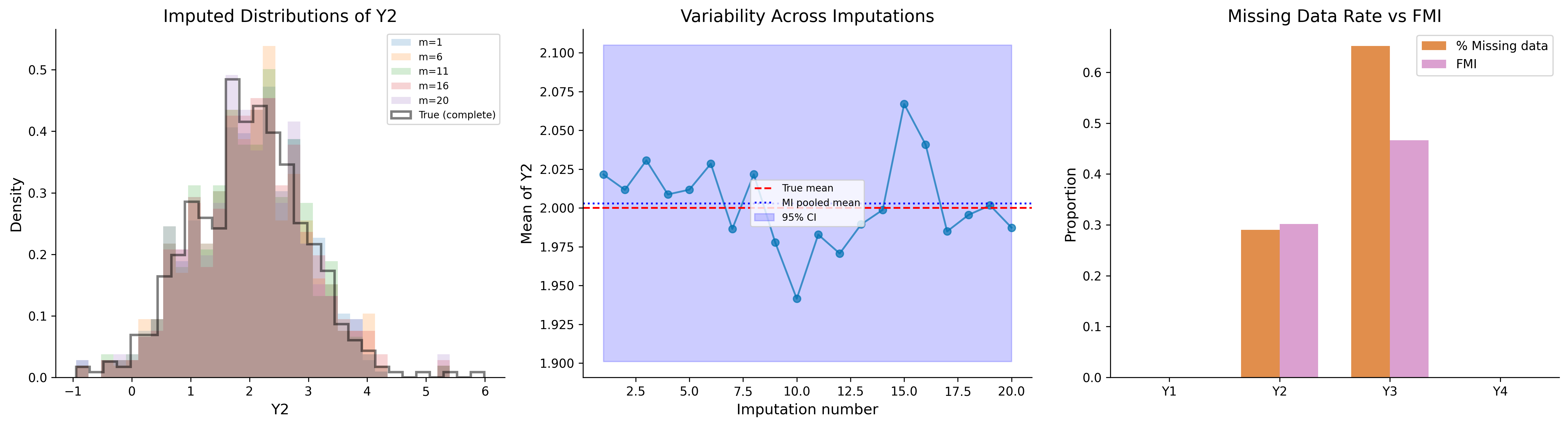
# Generate complete data and impose MARdata_mi, mu_mi, Sigma_mi = generate_multivariate_normal( n=500, p=4, rho=0.5, rng=rng)df_mi_mar, _ = impose_mar(data_mi, dep_col=0, miss_col=1, beta_mar=1.5, base_prob=0.3, rng=rng)# Also make col 2 MAR on col 0prob_col2 = expit(-0.3+1.0* data_mi[:, 0])mask_col2 = rng.random(500) < prob_col2df_mi_mar.iloc[mask_col2, 2] = np.nandf_mi_mar.columns = ['Y1', 'Y2', 'Y3', 'Y4']print(f"Missing data rates:")print(df_mi_mar.isnull().mean().round(3))# Run MICEmice = MICE(n_imputations=20, n_iterations=10, method='pmm', random_state=42)imputed_datasets = mice.fit_transform(df_mi_mar)# Analyze each dataset: estimate meansestimates = []variances = []for imp_data in imputed_datasets:ifisinstance(imp_data, pd.DataFrame): vals = imp_data.valueselse: vals = imp_data est = vals.mean(axis=0) var = vals.var(axis=0) /len(vals) estimates.append(est) variances.append(var)mi_results = rubins_rules(estimates, variances)print("\n"+"="*60)print("Multiple Imputation Results: Mean Estimation")print("="*60)print(f"\n{'Variable':>10s}{'True':>8s}{'MI est':>8s}{'MI SE':>8s} "f"{'CC est':>8s}{'FMI':>6s}")print("-"*55)for j inrange(4): cc_est = df_mi_mar.dropna().iloc[:, j].mean()print(f" Y{j+1}{mu_mi[j]:8.3f}{mi_results['estimate'][j]:8.3f} "f"{mi_results['se'][j]:8.3f}{cc_est:8.3f} "f"{mi_results['fmi'][j]:6.3f}")# Visualizationfig, axes = plt.subplots(1, 3, figsize=(18, 5))# Panel 1: Distribution of imputed values across m datasetsax = axes[0]for m_idx in [0, 5, 10, 15, 19]: imp = imputed_datasets[m_idx]ifisinstance(imp, pd.DataFrame): vals = imp.iloc[:, 1].valueselse: vals = imp[:, 1] ax.hist(vals, bins=30, alpha=0.2, density=True, label=f'm={m_idx+1}')ax.hist(data_mi[:, 1], bins=30, alpha=0.5, density=True, color='black', label='True (complete)', histtype='step', linewidth=2)ax.set_xlabel('Y2')ax.set_ylabel('Density')ax.set_title('Imputed Distributions of Y2')ax.legend(fontsize=8)# Panel 2: Trace plot of imputed means across iterationsax = axes[1]imp_means = [est[1] for est in estimates]ax.plot(range(1, len(imp_means) +1), imp_means, 'o-', color=colors[0], alpha=0.7)ax.axhline(mu_mi[1], color='red', linestyle='--', label='True mean')ax.axhline(mi_results['estimate'][1], color='blue', linestyle=':', label='MI pooled mean')ax.fill_between(range(1, len(imp_means) +1), mi_results['estimate'][1] -1.96* mi_results['se'][1], mi_results['estimate'][1] +1.96* mi_results['se'][1], alpha=0.2, color='blue', label='95% CI')ax.set_xlabel('Imputation number')ax.set_ylabel('Mean of Y2')ax.set_title('Variability Across Imputations')ax.legend(fontsize=8)# Panel 3: Fraction of missing informationax = axes[2]fmi = mi_results['fmi']pct_miss = df_mi_mar.isnull().mean().valuesx_pos = np.arange(4)width =0.35ax.bar(x_pos - width/2, pct_miss, width, label='% Missing data', color=colors[3], alpha=0.7)ax.bar(x_pos + width/2, fmi, width, label='FMI', color=colors[4], alpha=0.7)ax.set_xticks(x_pos)ax.set_xticklabels(['Y1', 'Y2', 'Y3', 'Y4'])ax.set_ylabel('Proportion')ax.set_title('Missing Data Rate vs FMI')ax.legend()plt.tight_layout()plt.show()
Missing data rates:
Y1    0.000
Y2    0.290
Y3    0.652
Y4    0.000
dtype: float64

============================================================
Multiple Imputation Results: Mean Estimation
============================================================

  Variable     True   MI est    MI SE   CC est    FMI
-------------------------------------------------------
  Y1         1.000    1.085    0.045    0.408  0.000
  Y2         2.000    2.003    0.052    1.788  0.302
  Y3         3.000    2.955    0.070    2.580  0.466
  Y4         4.000    4.003    0.045    3.700  0.000
MICE imputation diagnostics
57.8 Inverse Probability Weighting
57.8.1 Theory
Inverse Probability Weighting (IPW) reweights the observed data to represent the complete sample. The idea is that if we know (or can estimate) the probability that each observation is complete, we can upweight observations that are similar to those that are missing.
Let \(R_i = 1 - M_i\) be the response indicator (\(R_i = 1\) if observed, 0 if missing). Under MAR, the response probability (propensity) is:
The first term can be large when \(\pi_i\) is small (extreme weights), making IPW potentially inefficient. This motivates weight trimming and doubly robust methods.
IPW estimator implementation and comparison
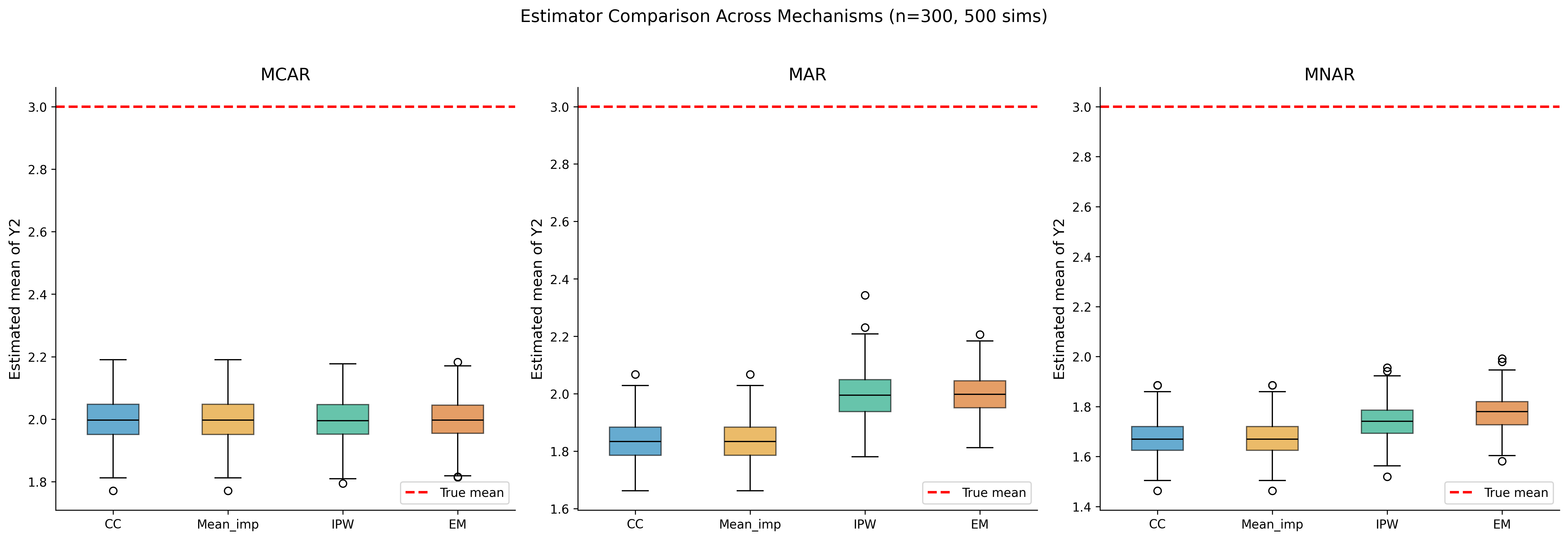
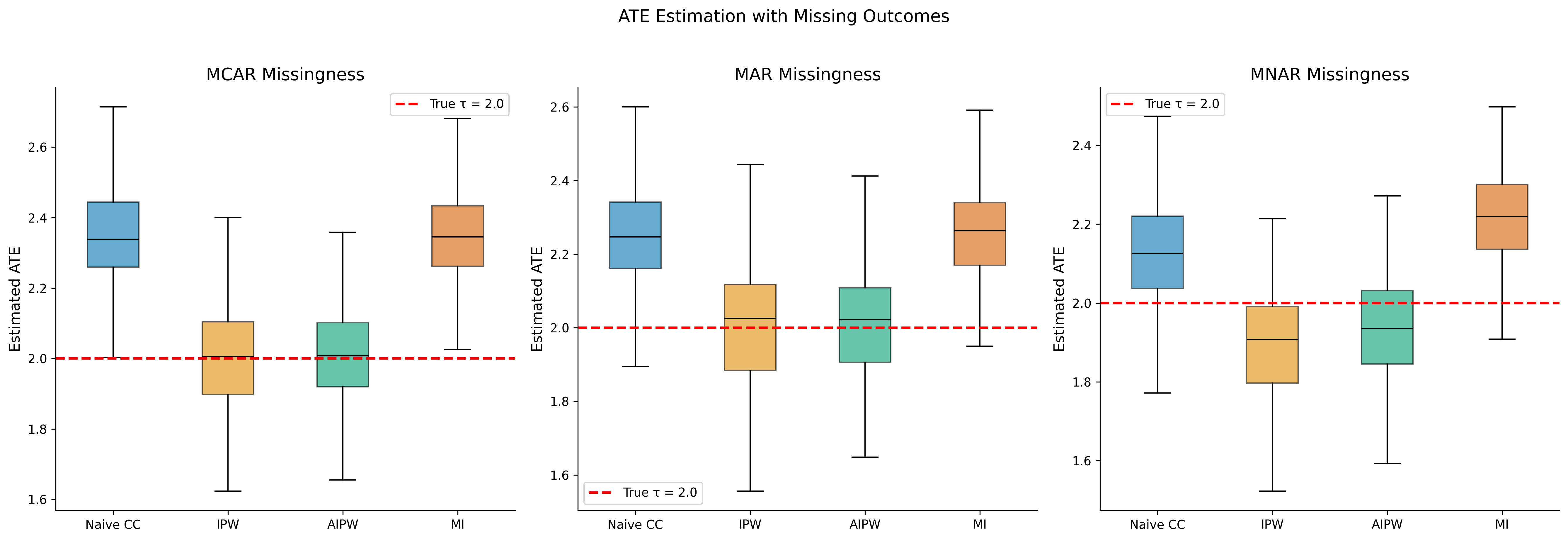
def ipw_estimator(Y, R, X, normalized=True):""" IPW estimator with logistic regression propensity model. Parameters ---------- Y : array Outcome (may contain NaN where R=0). R : array Response indicator (1=observed, 0=missing). X : array Covariates used to model missingness. normalized : bool If True, use Hajek (normalized) estimator. Returns ------- dict with estimate, se, weights """from sklearn.linear_model import LogisticRegression# Fit propensity modelif X.ndim ==1: X = X.reshape(-1, 1) lr = LogisticRegression(max_iter=1000, C=1e6) lr.fit(X, R) pi_hat = lr.predict_proba(X)[:, 1]# Clip to avoid extreme weights pi_hat = np.clip(pi_hat, 0.01, 0.99)# IPW estimate weights = R / pi_hat Y_obs = np.where(R ==1, Y, 0)if normalized: mu_hat = np.sum(weights * Y_obs) / np.sum(weights)else: mu_hat = np.mean(weights * Y_obs)# Variance estimation (sandwich)if normalized: resid = R * (Y_obs - mu_hat) / pi_hat se = np.sqrt(np.var(resid) /len(Y))else: se = np.sqrt(np.var(weights * Y_obs) /len(Y))return {'estimate': mu_hat,'se': se,'weights': weights[R ==1],'propensity': pi_hat }# Simulation: compare methods under three mechanismsn_sim =500true_mean =3.0# mu_true[1] for Y2results_by_mechanism = {}for mech_name, impose_fn in [ ('MCAR', lambda d, r: impose_mcar(d, 0.3, [1], r)), ('MAR', lambda d, r: impose_mar(d, 0, 1, 1.5, 0.3, r)), ('MNAR', lambda d, r: impose_mnar(d, 1, 1.5, 0.3, r))]: estimates = {'CC': [], 'Mean_imp': [], 'IPW': [], 'EM': []}for sim inrange(n_sim): sim_rng = np.random.default_rng(sim) data_sim, _, _ = generate_multivariate_normal( n=300, p=4, rho=0.5, rng=sim_rng )if mech_name =='MCAR': df_sim = impose_fn(data_sim, sim_rng) true_probs =Noneelse: df_sim, true_probs = impose_fn(data_sim, sim_rng) R = (~df_sim.iloc[:, 1].isna()).astype(int).values# Complete case estimates['CC'].append(df_sim.iloc[:, 1].mean())# Mean imputation mean_val = df_sim.iloc[:, 1].mean() estimates['Mean_imp'].append(mean_val)# IPWtry: ipw_res = ipw_estimator( data_sim[:, 1], R, data_sim[:, 0], normalized=True ) estimates['IPW'].append(ipw_res['estimate'])exceptException: estimates['IPW'].append(np.nan)# EMtry: em_res = em_mvn(df_sim, max_iter=100) estimates['EM'].append(em_res['mu'][1])exceptException: estimates['EM'].append(np.nan) results_by_mechanism[mech_name] = { k: np.array(v) for k, v in estimates.items() }# Visualizationfig, axes = plt.subplots(1, 3, figsize=(18, 6))for ax, mech_name inzip(axes, ['MCAR', 'MAR', 'MNAR']): res = results_by_mechanism[mech_name] methods =list(res.keys()) data_plot = [res[m][~np.isnan(res[m])] for m in methods] bp = ax.boxplot(data_plot, labels=methods, patch_artist=True, medianprops=dict(color='black'))for patch, color inzip(bp['boxes'], colors[:4]): patch.set_facecolor(color) patch.set_alpha(0.6) ax.axhline(true_mean, color='red', linestyle='--', linewidth=2, label='True mean') ax.set_title(f'{mech_name}') ax.set_ylabel('Estimated mean of Y2') ax.legend()plt.suptitle(f'Estimator Comparison Across Mechanisms (n=300, {n_sim} sims)', fontsize=14, y=1.02)plt.tight_layout()plt.show()# Print bias and RMSE tableprint("\n"+"="*75)print(f"{'':12s}{'MCAR':>20s}{'MAR':>20s}{'MNAR':>20s}")print(f"{'Method':12s}{'Bias':>8s}{'RMSE':>8s}{'Bias':>8s} "f"{'RMSE':>8s}{'Bias':>8s}{'RMSE':>8s}")print("-"*75)for method in ['CC', 'Mean_imp', 'IPW', 'EM']: row =f"{method:12s}"for mech in ['MCAR', 'MAR', 'MNAR']: vals = results_by_mechanism[mech][method] vals = vals[~np.isnan(vals)] bias = np.mean(vals) - true_mean rmse = np.sqrt(np.mean((vals - true_mean)**2)) row +=f" {bias:8.4f}{rmse:8.4f} "print(row)
IPW estimation under different missingness mechanisms
57.9.1 Augmented Inverse Probability Weighting (AIPW)
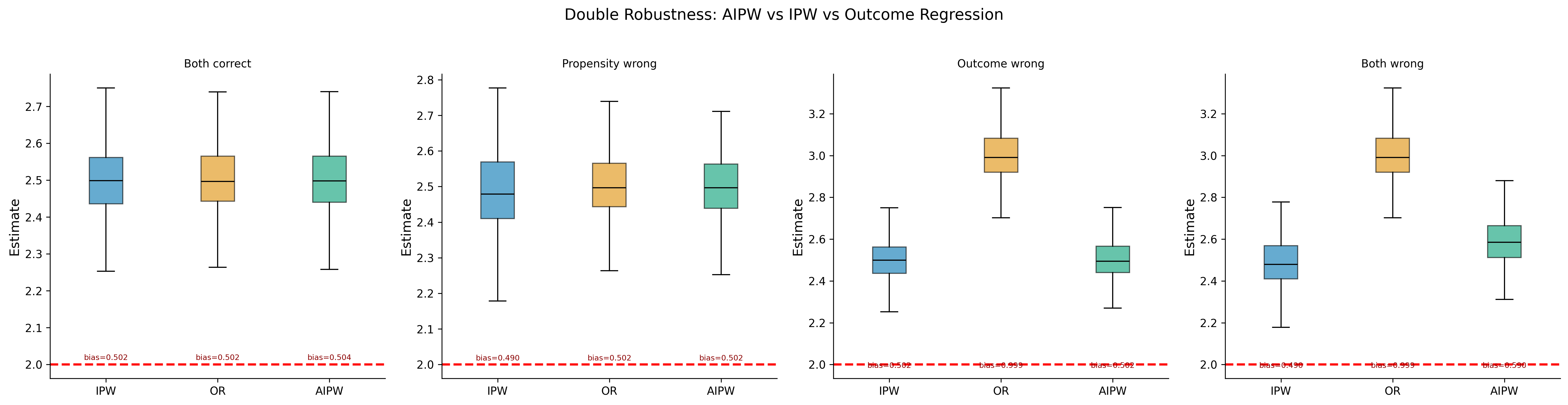
The Augmented IPW (AIPW) estimator (Robins, Rotnitzky, and Zhao 1994; Scharfstein, Rotnitzky, and Robins 1999) combines the IPW estimator with an outcome regression model. It has the double robustness property: it is consistent if either the propensity model or the outcome model is correctly specified (but not necessarily both).
Even if \(\hat{\pi} \neq \pi\), the term \(E[Y_i - m(X_i) \mid X_i] = 0\), so the IPW correction vanishes in expectation, and \(\hat{\mu}_{\text{AIPW}} \to E[m(X)] = E[Y]\).
Case 2: Propensity model correct (\(\hat{\pi}(X_i) = \pi(X_i)\)). Then even if \(\hat{m}\) is wrong:
When both models are correct, AIPW achieves the semiparametric efficiency bound(Tsiatis 2006), meaning no regular asymptotically linear estimator can have lower asymptotic variance.
Causal inference involves a fundamental missing data problem: for each unit, we observe at most one potential outcome. When actual data missingness is superimposed on this, we have a double missing data problem(Ding and Li 2018):
Fundamental problem of causal inference: For unit \(i\) with treatment \(D_i\), we observe \(Y_i = D_i Y_i(1) + (1 - D_i) Y_i(0)\); the counterfactual \(Y_i(1 - D_i)\) is always missing.
Survey/measurement missingness: Even the observed potential outcome \(Y_i(D_i)\) may be missing in the data.
The interaction between these two sources of missingness creates novel identification challenges.
57.10.2 Treatment Effect Estimation with Missing Outcomes
Consider estimating the Average Treatment Effect \(\tau = E[Y(1) - Y(0)]\) when the outcome \(Y\) is subject to missingness. Let \(R_i\) indicate whether \(Y_i\) is observed.
Assumptions:
Unconfoundedness (for causal identification):\((Y(0), Y(1)) \perp\!\!\!\perp D \mid X\)
MAR for missingness:\(R \perp\!\!\!\perp Y \mid X, D\)
Under these assumptions, the AIPW estimator for the ATE becomes:
\(\hat{e}(X_i) = \hat{P}(D = 1 \mid X_i)\) is the treatment propensity.
\(\hat{\pi}_d(X_i) = \hat{P}(R = 1 \mid D = d, X_i)\) is the response propensity.
\(\hat{\mu}_d(X_i) = \hat{E}[Y \mid D = d, X_i]\) is the outcome model.
This estimator is triply robust in the sense that it is consistent if any two of the three models (treatment propensity, response propensity, outcome model) are correctly specified (Sun et al. 2018).
Simulation: Treatment effect estimation with missing outcomes
A distinct and arguably harder problem arises when covariates (confounders) are missing rather than the outcome. If a confounder \(X_j\) required for the unconfoundedness assumption is missing for some units, then:
Complete-case analysis may be valid if missingness in \(X_j\) is independent of treatment and potential outcomes conditional on observed covariates (a strong assumption).
MI can be used to impute \(X_j\), but the imputation model must be congenial with the analysis model-it should include the outcome, treatment, and all other confounders as predictors (Meng 1994).
Mayer et al. (2020) propose a doubly robust approach that combines imputation and weighting for missing confounders.
Critical insight (Sullivan et al. (2018)): When imputing covariates for causal inference, the imputation model must include the outcome and the treatment indicator. Omitting these violates congeniality and leads to biased treatment effect estimates, even under MAR for the covariates.
57.11 Missing Data for Prediction
57.11.1 Prediction vs. Inference: Different Goals, Different Methods
When the goal is prediction rather than inference about structural parameters, the considerations shift:
Bias is less important relative to variance. A slightly biased predictor with lower MSE may be preferred.
We must handle missingness at both training and test/deployment time. The prediction model must accommodate missing inputs.
The missingness mechanism at test time may differ from training time.
57.11.2 Approaches for Prediction with Missing Data
1. Impute-then-predict:
Impute training data (single or multiple imputation), fit model on completed data, and at test time impute missing features before prediction.
Risk: Imputation errors propagate; imputation model and prediction model may be poorly coordinated.
2. Native handling in tree-based models:
Modern gradient boosting implementations (XGBoost, LightGBM, CatBoost) handle missing values natively by learning optimal split directions for missing inputs. This avoids separate imputation entirely.
XGBoost: At each split, missing values are sent to the child that minimizes the loss. The direction is learned from data.
This approach is robust to missingness mechanisms and often outperforms impute-then-predict pipelines.
3. MissForest and iterative imputation:
Stekhoven and Bühlmann (2012) proposed using random forests for iterative imputation, analogous to MICE but with nonparametric models. The procedure:
Initialize missing values.
For each variable (sorted by missingness amount): fit a random forest on observed values using all other variables as predictors, then predict missing values.
Iterate until convergence.
4. Embedding-based approaches:
For neural network models, missing indicators can be concatenated with the feature vector, and the network learns to handle missingness implicitly. Ipsen, Mattei, and Frellsen (2022) survey deep learning approaches for missing data.
Comparison of prediction methods with missing data
Prediction performance under different missingness rates and mechanisms
57.12 Sensitivity Analysis for MNAR
57.12.1 The Fundamental Challenge
Under MNAR, the missingness mechanism is nonignorable and standard methods (MI, EM, IPW under MAR) produce biased results. Since MNAR cannot be tested from observed data alone, sensitivity analysis is the recommended approach: conduct the primary analysis under MAR, then systematically vary assumptions about the MNAR departure and examine how conclusions change.
57.12.2 Pattern Mixture Models
Pattern Mixture Models (PMMs)(R. J. A. Little 1993) decompose the joint distribution of \((Y, M)\) by conditioning on the missing data pattern:
\[
f(Y, M) = f(Y \mid M) \cdot f(M)
\]
This contrasts with selection models, which factor as \(f(Y) \cdot f(M \mid Y)\).
In a PMM, we specify a separate model for \(Y\) within each missing data pattern. The overall distribution is a mixture:
\[
f(Y) = \sum_m f(Y \mid M = m) \cdot P(M = m)
\]
The challenge is that \(f(Y \mid M = m)\) for patterns \(m\) with missing components is not identified from observed data. Sensitivity analysis proceeds by specifying identifying restrictions:
Complete Case Missing Values (CCMV): The conditional distribution of the missing variables given the observed variables is the same as in the complete-case pattern.
Neighboring Case Missing Values (NCMV): The distribution is borrowed from the next less-missing pattern.
Available Case Missing Values (ACMV): Uses observed data from all patterns where the variable is observed.
\(\delta\)-adjustment: Shift the distribution of \(Y_{\text{mis}}\) by a sensitivity parameter \(\delta\):
\[
f(Y_{\text{mis}} \mid Y_{\text{obs}}, M = m) = f(Y_{\text{mis}} \mid Y_{\text{obs}}, M = m_{\text{ref}}) \cdot \exp(\delta Y_{\text{mis}}) / C(\delta)
\]
57.12.3 Tipping Point Analysis
Tipping point analysis systematically varies the sensitivity parameter \(\delta\) to find the value at which the substantive conclusion changes (e.g., a treatment effect becomes nonsignificant or changes sign).
Sensitivity analysis for MNAR using delta-adjustment
def tipping_point_analysis(Y, D, X, R, delta_range, n_mi=20, rng=None):""" Tipping point analysis for treatment effect under MNAR. For each delta value, shift imputed values for missing outcomes by delta and re-estimate the treatment effect. Under MAR, delta = 0. Under MNAR, delta != 0 means missing outcomes are systematically higher (delta > 0) or lower (delta < 0) than what MAR would predict. """if rng isNone: rng = np.random.default_rng() results = []for delta in delta_range: tau_estimates = []for m inrange(n_mi):# Impute under MAR first X_full = np.column_stack([X, D]) lm = LinearRegression() lm.fit(X_full[R ==1], Y[R ==1]) pred_miss = lm.predict(X_full[R ==0]) resid_var = np.var(Y[R ==1] - lm.predict(X_full[R ==1]))# Draw imputed values with delta shift Y_imp = Y.copy() Y_imp[R ==0] = pred_miss + rng.normal(0, np.sqrt(resid_var), (R ==0).sum()) + delta# Estimate ATE with OLS X_ate = np.column_stack([D, X]) lm_ate = LinearRegression() lm_ate.fit(X_ate, Y_imp) tau_estimates.append(lm_ate.coef_[0]) tau_arr = np.array(tau_estimates) tau_mean = np.mean(tau_arr) tau_se = np.sqrt(np.var(tau_arr) + np.mean([ np.var(Y) /len(Y)] * n_mi)) # Simplified SE results.append({'delta': delta,'tau': tau_mean,'se': np.std(tau_arr),'lower': tau_mean -1.96* np.std(tau_arr),'upper': tau_mean +1.96* np.std(tau_arr),'p_value': 2* (1- stats.norm.cdf(abs(tau_mean) / (np.std(tau_arr) +1e-10))) })return pd.DataFrame(results)# Generate data with MNAR missingnessn_sens =1000dgp_sens = generate_treatment_dgp(n=n_sens, tau=2.0, rng=rng)X_s, D_s, Y_s = dgp_sens['X'], dgp_sens['D'], dgp_sens['Y']# MNAR: sicker patients (lower Y) more likely missingmiss_prob = expit(1.0-0.8* Y_s)R_s = (rng.random(n_sens) > miss_prob).astype(int)print(f"Missing rate: {1- R_s.mean():.2%}")print(f"True ATE: 2.0")print(f"Naive CC estimate: "f"{Y_s[R_s==1][D_s[R_s==1]==1].mean() - Y_s[R_s==1][D_s[R_s==1]==0].mean():.3f}")# Tipping point analysisdeltas = np.linspace(-3, 3, 31)tp_results = tipping_point_analysis(Y_s, D_s, X_s, R_s, deltas, n_mi=20, rng=rng)# Plotfig, axes = plt.subplots(1, 2, figsize=(14, 6))# Panel 1: Tipping point plotax = axes[0]ax.plot(tp_results['delta'], tp_results['tau'], 'b-', linewidth=2, label='Estimated ATE')ax.fill_between(tp_results['delta'], tp_results['lower'], tp_results['upper'], alpha=0.2, color='blue', label='95% CI')ax.axhline(0, color='gray', linestyle=':', alpha=0.5)ax.axhline(2.0, color='red', linestyle='--', alpha=0.7, label='True ATE = 2.0')ax.axvline(0, color='green', linestyle=':', alpha=0.5, label='MAR (δ=0)')ax.set_xlabel('Sensitivity parameter δ\n(δ > 0: missing Y higher than predicted)')ax.set_ylabel('Estimated ATE')ax.set_title('Tipping Point Analysis')ax.legend(fontsize=9)# Find tipping point (where CI includes 0)tp_idx =Nonefor i, row in tp_results.iterrows():if row['lower'] <=0<= row['upper']: tp_idx = ibreakif tp_idx isnotNone: ax.axvline(tp_results.loc[tp_idx, 'delta'], color='purple', linestyle='--', alpha=0.7) ax.annotate(f'Tipping point\nδ ≈ {tp_results.loc[tp_idx, "delta"]:.1f}', xy=(tp_results.loc[tp_idx, 'delta'], 0), xytext=(tp_results.loc[tp_idx, 'delta'] -1.5, -1), arrowprops=dict(arrowstyle='->', color='purple'), fontsize=10, color='purple')# Panel 2: P-value as function of deltaax = axes[1]ax.plot(tp_results['delta'], tp_results['p_value'], 'r-', linewidth=2)ax.axhline(0.05, color='gray', linestyle='--', alpha=0.5, label='α = 0.05')ax.set_xlabel('Sensitivity parameter δ')ax.set_ylabel('p-value')ax.set_title('Statistical Significance Under MNAR')ax.set_ylim(-0.05, 1.05)ax.legend()plt.tight_layout()plt.show()print("\nInterpretation:")if tp_idx isnotNone:print(f" The treatment effect remains significant for "f"δ ∈ [{tp_results['delta'].iloc[0]:.1f}, "f"{tp_results.loc[tp_idx, 'delta']:.1f})")print(f" The tipping point is δ ≈ {tp_results.loc[tp_idx, 'delta']:.1f}")print(f" This means: if missing outcomes are systematically "f"{abs(tp_results.loc[tp_idx, 'delta']):.1f} units")print(f" {'higher'if tp_results.loc[tp_idx, 'delta'] <0else'lower'} "f"than MAR predicts, the ATE becomes non-significant.")
Missing rate: 36.80%
True ATE: 2.0
Naive CC estimate: 2.112
Tipping point analysis: How ATE changes under MNAR departures
Interpretation:
57.13 Advanced Methods
57.13.1 Deep Learning Approaches
Recent advances in deep generative modeling have introduced powerful new approaches to missing data imputation:
GAIN adapts the GAN framework for missing data imputation. The generator takes incomplete data and noise as input and produces completed data. The discriminator tries to distinguish which components were originally observed versus imputed. The key innovation is a hint mechanism that provides partial information about the missingness mask to the discriminator, preventing mode collapse.
MIWAE uses a variational autoencoder (VAE) framework with importance weighting for missing data. The model maximizes a tighter lower bound on the observed-data log-likelihood:
The advantage of MIWAE over standard VAEs is that it handles missing data in the observation model directly, producing well-calibrated uncertainty estimates.
Extends MIWAE to handle MNAR data by jointly modeling the data and the missingness mechanism. The model includes a missingness network that parametrizes \(P(M \mid X, Z)\) where \(Z\) is the latent variable.
57.13.2 Optimal Transport for Missing Data
Muzellec et al. (2020) proposed using optimal transport theory for missing data imputation. The key idea is to find the imputation that minimizes the Wasserstein distance between the imputed distribution and a target distribution.
For two distributions \(P\) and \(Q\) with supports in \(\mathbb{R}^p\), the 2-Wasserstein distance is:
The imputation is found by minimizing \(S_\epsilon(\hat{P}_{\text{imputed}}, \hat{P}_{\text{target}})\) where \(\hat{P}_{\text{target}}\) is estimated from observed data.
57.13.3 MissForest: Random Forest Imputation
Stekhoven and Bühlmann (2012) proposed a nonparametric imputation method based on random forests:
MissForest implementation
class MissForest:""" Random forest-based iterative imputation (Stekhoven & Bühlmann, 2012). Parameters ---------- max_iter : int Maximum number of iterations. n_estimators : int Number of trees in each random forest. random_state : int Random seed. """def__init__(self, max_iter=10, n_estimators=100, random_state=42):self.max_iter = max_iterself.n_estimators = n_estimatorsself.random_state = random_statedef fit_transform(self, data):"""Impute missing values using iterative random forest."""ifisinstance(data, pd.DataFrame): X = data.values.copy() columns = data.columnselse: X = data.copy() columns =None n, p = X.shape miss_mask = np.isnan(X)# Initialize with column means X_imp = X.copy() col_means = np.nanmean(X, axis=0)for j inrange(p): X_imp[miss_mask[:, j], j] = col_means[j]# Sort columns by missingness (least to most) miss_count = miss_mask.sum(axis=0) col_order = np.argsort(miss_count) cols_to_impute = [j for j in col_order if miss_count[j] >0] prev_imp = X_imp.copy()for iteration inrange(self.max_iter):for j in cols_to_impute: obs_rows =~miss_mask[:, j] mis_rows = miss_mask[:, j]if mis_rows.sum() ==0:continue other_cols = [c for c inrange(p) if c != j]# Fit random forest on observed data rf = RandomForestRegressor( n_estimators=self.n_estimators, random_state=self.random_state + iteration *100+ j, n_jobs=-1 ) rf.fit(X_imp[obs_rows][:, other_cols], X[obs_rows, j])# Predict missing values X_imp[mis_rows, j] = rf.predict( X_imp[mis_rows][:, other_cols])# Check convergence diff = np.sum((X_imp - prev_imp)**2) total = np.sum(X_imp**2)if total >0and diff / total <1e-6:break prev_imp = X_imp.copy()if columns isnotNone:return pd.DataFrame(X_imp, columns=columns)return X_imp# Test MissForestmf = MissForest(max_iter=5, n_estimators=50, random_state=42)data_mf, mu_mf, _ = generate_multivariate_normal( n=500, p=4, rho=0.5, rng=rng)df_mf_mar, _ = impose_mar(data_mf, dep_col=0, miss_col=1, beta_mar=1.5, rng=rng)df_mf_mar.columns = ['Y1', 'Y2', 'Y3', 'Y4']imputed_mf = mf.fit_transform(df_mf_mar)print("MissForest Imputation Results:")print(f" True mean: {mu_mf.round(4)}")print(f" MissForest mean: {imputed_mf.mean().values.round(4)}")print(f" Complete-case: {df_mf_mar.dropna().mean().values.round(4)}")
We now conduct a comprehensive Monte Carlo study comparing all methods discussed across all missingness mechanisms, sample sizes, and missing data fractions.
Comprehensive simulation comparing all methods
def comprehensive_simulation(n_sims=200, rng_base=42):""" Monte Carlo study comparing methods across scenarios. """ scenarios = []for n in [200, 1000]:for miss_rate in [0.1, 0.3, 0.5]:for mechanism in ['MCAR', 'MAR', 'MNAR']: scenarios.append({'n': n, 'miss_rate': miss_rate, 'mechanism': mechanism }) methods = ['CC', 'Mean', 'EM', 'MI_PMM', 'MissForest'] all_results = []for scenario in scenarios: n = scenario['n'] miss_rate = scenario['miss_rate'] mechanism = scenario['mechanism'] estimates = {m: [] for m in methods}for sim inrange(n_sims): sim_rng = np.random.default_rng(rng_base + sim) data_sim, mu_sim, _ = generate_multivariate_normal( n=n, p=4, rho=0.5, rng=sim_rng) true_mean_y2 = mu_sim[1]# Impose missingnessif mechanism =='MCAR': df_sim = impose_mcar(data_sim, miss_rate, [1], sim_rng)elif mechanism =='MAR': df_sim, _ = impose_mar(data_sim, 0, 1, 1.5, miss_rate, sim_rng)else: df_sim, _ = impose_mnar(data_sim, 1, 1.5, miss_rate, sim_rng) df_sim.columns = ['Y1', 'Y2', 'Y3', 'Y4']# CC estimates['CC'].append(df_sim['Y2'].mean())# Mean imputation estimates['Mean'].append(df_sim['Y2'].mean())# EMtry: em_r = em_mvn(df_sim, max_iter=100) estimates['EM'].append(em_r['mu'][1])exceptException: estimates['EM'].append(np.nan)# MI (PMM)try: mice_obj = MICE(n_imputations=10, n_iterations=5, method='pmm', random_state=sim) imp_dsets = mice_obj.fit_transform(df_sim) mi_ests = [d['Y2'].mean() ifisinstance(d, pd.DataFrame) else d[:, 1].mean() for d in imp_dsets] estimates['MI_PMM'].append(np.mean(mi_ests))exceptException: estimates['MI_PMM'].append(np.nan)# MissForesttry: mf_obj = MissForest(max_iter=3, n_estimators=30, random_state=sim) mf_imp = mf_obj.fit_transform(df_sim)ifisinstance(mf_imp, pd.DataFrame): estimates['MissForest'].append(mf_imp['Y2'].mean())else: estimates['MissForest'].append(mf_imp[:, 1].mean())exceptException: estimates['MissForest'].append(np.nan)for method in methods: vals = np.array(estimates[method]) vals = vals[~np.isnan(vals)]iflen(vals) >0: all_results.append({'n': n,'miss_rate': miss_rate,'mechanism': mechanism,'method': method,'bias': np.mean(vals) - true_mean_y2,'rmse': np.sqrt(np.mean((vals - true_mean_y2)**2)),'se': np.std(vals),'coverage_proxy': np.mean( np.abs(vals - true_mean_y2) <1.96* np.std(vals)) })return pd.DataFrame(all_results)print("Running comprehensive simulation (this may take a few minutes)...")comp_results = comprehensive_simulation(n_sims=100, rng_base=42)print("Done!")# Heatmap of biasfig, axes = plt.subplots(2, 3, figsize=(18, 10))for row, n_val inenumerate([200, 1000]):for col, mech inenumerate(['MCAR', 'MAR', 'MNAR']): ax = axes[row, col] subset = comp_results[ (comp_results['n'] == n_val) & (comp_results['mechanism'] == mech) ]# Pivot for heatmap pivot_bias = subset.pivot( index='method', columns='miss_rate', values='bias' )# Reorder method_order = ['CC', 'Mean', 'EM', 'MI_PMM', 'MissForest'] pivot_bias = pivot_bias.reindex(method_order) im = ax.imshow(pivot_bias.values, cmap='RdBu_r', vmin=-0.5, vmax=0.5, aspect='auto') ax.set_xticks(range(len(pivot_bias.columns))) ax.set_xticklabels([f'{r:.0%}'for r in pivot_bias.columns]) ax.set_yticks(range(len(pivot_bias.index))) ax.set_yticklabels(pivot_bias.index)# Annotatefor i inrange(len(pivot_bias.index)):for j inrange(len(pivot_bias.columns)): val = pivot_bias.iloc[i, j] ax.text(j, i, f'{val:.3f}', ha='center', va='center', fontsize=8, color='white'ifabs(val) >0.3else'black') ax.set_title(f'{mech}, n={n_val}')if col ==0: ax.set_ylabel('Method')if row ==1: ax.set_xlabel('Missing Rate')plt.suptitle('Bias Across Methods, Mechanisms, and Sample Sizes', fontsize=14, y=1.02)plt.colorbar(im, ax=axes, shrink=0.6, label='Bias')plt.tight_layout()plt.show()
Running comprehensive simulation (this may take a few minutes)...
Done!
57.15 Structural Parameters vs. Prediction: A Unified View
57.15.1 When Does the Purpose Matter?
The distinction between causal inference (structural parameters) and prediction determines:
Which missingness assumptions matter:
For structural parameters (e.g., ATE, regression coefficients with causal interpretation): we need consistent estimators, so the missingness mechanism must be correctly addressed. MAR vs. MNAR determines whether standard methods are valid.
For prediction: we need low test-set MSE. If the missingness pattern at test time is similar to training time, even biased imputation methods (mean imputation) can work well because the bias may be absorbed by the prediction model.
Prediction: prioritize low MSE = bias² + variance. A biased-but-stable method (e.g., regularized regression with mean imputation) may outperform an unbiased-but-noisy method (e.g., AIPW with estimated propensities).
Whether to model the missingness mechanism explicitly:
Causal inference: Yes-IPW and AIPW explicitly model the response propensity; MNAR requires sensitivity analysis.
Prediction: Often not necessary-tree-based methods with native NaN handling or imputation with missingness indicators capture the information content of missingness without explicit mechanism modeling.
Unified comparison: structural parameter vs prediction
The purpose of the analysis matters for method selection
57.16 Practical Guidelines and Decision Framework
57.16.1 Decision Tree for Method Selection
Based on the theoretical results and simulation evidence presented in this chapter, we propose the following decision framework:
Step 1: Characterize the missingness.
Examine missing data patterns (monotone vs. nonmonotone).
Run Little’s MCAR test and auxiliary variable analyses.
Use substantive knowledge to assess plausibility of MAR.
Step 2: Determine the analytical goal.
If causal inference / structural parameters: prioritize consistency. Use MI, FIML/EM, or AIPW. Conduct sensitivity analysis for MNAR.
If prediction: prioritize test-set performance. Consider native NaN handling (XGBoost/LightGBM), mean imputation with missingness indicators, or MissForest.
Step 3: Select method(s).
Scenario
Recommended Primary
Recommended Robustness Check
MCAR, any goal
Any method works; MI or FIML for efficiency
Complete-case as benchmark
MAR, structural parameters
MI (MICE with PMM) or FIML
AIPW (doubly robust)
MAR, prediction
Native NaN handling or MissForest
Mean imp + indicators
MNAR suspected, structural
MI under MAR + sensitivity analysis
Pattern mixture models, tipping point
MNAR suspected, prediction
Native NaN handling
Compare with MAR-imputed
High missing fraction (>50%)
MI with many imputations (\(m \geq 50\))
Reconsider data collection
Monotone pattern
MI or EM (efficient)
LOCF sensitivity (clinical)
Step 4: Validate and report.
Compare results across methods. Large discrepancies signal sensitivity to assumptions.
Report the fraction of missing information (FMI), not just the missing data rate.
For causal inference, always conduct and report sensitivity analysis for MNAR.
57.16.2 Common Pitfalls
Using mean imputation for anything other than prediction. It attenuates variances, correlations, and standard errors.
Omitting the outcome from the MI imputation model. This leads to attenuated estimates of associations (violation of congeniality).
Using too few imputations. With modern computing, \(m \geq 20\) is easy and recommended.
Treating MAR as testable. It is not; use sensitivity analysis.
Ignoring missing data in covariates. Even 5% missingness in a key confounder can bias treatment effects.
Assuming MCAR when it’s implausible. Most real-world missingness is at least MAR.
Not accounting for auxiliary variables. Including variables predictive of missingness in the imputation model (even if not in the analysis model) improves MI.
Applying LOCF as a primary method. It is generally biased under MAR and MNAR.
57.17 Connections to Related Fields
57.17.1 Missing Data and Survey Sampling
Survey nonresponse is a missing data problem where the “missingness mechanism” is the nonresponse mechanism. The propensity score methods of Rosenbaum and Rubin (1983) for causal inference directly parallel the response propensity models used in survey weighting. Kalton and Kasprzyk (1986) and R. J. A. Little (1986) provide foundational treatments of this connection.
57.17.2 Missing Data and Measurement Error
Missing data and measurement error are fundamentally related. Buonaccorsi (2010) notes that a variable measured with error can be viewed as having a “partial missing” data problem: the true value is missing, and we observe a noisy proxy. Methods from both literatures (EM algorithm, MI, structural equation modeling) apply to both problems.
57.17.3 Missing Data and Causal Mediation
In causal mediation analysis, the direct and indirect effects involve counterfactual mediator values that are never observed-a missing data problem. When actual missingness is superimposed, the identification conditions become more complex. Tchetgen Tchetgen and Shpitser (2012) develop semiparametric methods for mediation with missing data.
57.17.4 Missing Data in Panel/Longitudinal Settings
Mixed-effects models estimated with FIML (equivalent to MAR assumption).
Generalized Estimating Equations (GEE) with inverse probability of censoring weighting (IPCW).
Joint models for longitudinal and time-to-event data, which model the dropout process jointly with the outcome trajectory (Rizopoulos 2012).
57.18 Applied Examples
We now ground the theory in three substantive domains where missing data arises naturally, each with distinct mechanisms, stakes, and analytical goals. All data are simulated to illustrate the mechanisms transparently-but the DGPs are calibrated to reflect realistic feature distributions and missingness patterns documented in applied research.
57.18.1 Example 1: Credit Scoring with Missing Income Data
57.18.1.1 Context and Motivation
Credit scoring is a canonical prediction problem where missing data is pervasive and consequential. In consumer lending markets, applicants frequently have missing income documentation, missing employment history, or missing prior credit records. The missingness is almost certainly not MCAR: higher-income applicants with formal sector employment are more likely to have verifiable income documentation, while informal sector workers (street vendors, freelance workers, agricultural laborers) often cannot produce pay stubs or tax filings. This creates a selection problem that directly affects both the fairness and accuracy of credit models.
Two analytical goals coexist:
Prediction: The lender wants to predict default probability \(P(\text{default} \mid X)\) as accurately as possible to make lending decisions. Here, minimizing out-of-sample log-loss or Brier score is the objective.
Causal inference: A regulator or policy researcher wants to estimate the causal effect of credit access on household consumption or the structural relationship between income and default. Here, consistency of the estimated coefficient matters-biased estimates lead to incorrect policy conclusions about, e.g., whether expanding credit to informal workers increases or decreases systemic risk.
57.18.1.2 Data Generating Process
We simulate a credit market with realistic feature dependencies:
Credit scoring DGP with realistic missingness
def generate_credit_data(n=5000, rng=None):""" Simulate consumer credit data. Features: - age: applicant age (22-65) - income: monthly income in million VND (log-normal) - employment_type: 0=informal, 1=formal sector - credit_history_length: months of credit history (0 = no history) - loan_amount: requested loan in million VND - debt_to_income: existing debt / income ratio Outcome: - default: 1 if borrower defaults within 12 months Missingness: - income: MNAR (high earners less likely to be missing, but informal workers also less likely to have documentation) - credit_history_length: MAR (depends on age and employment type) - debt_to_income: MNAR (those with high DTI avoid reporting) """if rng isNone: rng = np.random.default_rng(42)# --- Generate complete data --- age = rng.uniform(22, 65, n) employment_type = rng.binomial(1, expit(-1.5+0.04* age), n)# Income depends on age and employment (log-normal) log_income = (1.8+0.015* age +0.6* employment_type +0.3* rng.standard_normal(n)) income = np.exp(log_income) # million VND# Credit history: formal employees have longer histories credit_history = np.maximum(0, -12+0.8* age +24* employment_type + rng.normal(0, 18, n) ).astype(int)# Loan amount loan_amount = income * rng.uniform(1, 8, n)# Debt-to-income ratio dti = np.maximum(0, 0.15+0.1* (1- employment_type) + rng.exponential(0.15, n))# Default probability (true structural model)# Key structural parameter: beta_income = -0.4 # (higher income causally reduces default probability) latent_default = (1.5-0.4* np.log(income) # structural parameter of interest+0.8* dti # higher DTI -> more default-0.02* age # older -> less default-0.5* employment_type # formal -> less default-0.01* credit_history # longer history -> less default+0.1* np.log(loan_amount) # larger loan -> more default+ rng.logistic(0, 1, n) # logistic error ) default = (latent_default >0).astype(int) df_complete = pd.DataFrame({'age': age,'income': income,'employment_type': employment_type,'credit_history': credit_history,'loan_amount': loan_amount,'dti': dti,'default': default })# --- Impose realistic missingness --- df_missing = df_complete.copy()# 1. Income: MNAR# Informal workers less likely to have docs; # also those with extreme incomes less likely to report p_miss_income = expit(0.5-1.5* employment_type # formal workers have docs-0.3* np.log(income) # MNAR: depends on income itself+0.02* age # older slightly less likely to report ) mask_income = rng.random(n) < p_miss_income df_missing.loc[mask_income, 'income'] = np.nan# 2. Credit history: MAR (depends on age and employment) p_miss_credit = expit(1.0-0.03* age # younger -> more missing-0.8* employment_type # informal -> more missing ) mask_credit = rng.random(n) < p_miss_credit df_missing.loc[mask_credit, 'credit_history'] = np.nan# 3. DTI: MNAR (high DTI applicants avoid reporting) p_miss_dti = expit(-2.0+3.0* dti) # MNAR: depends on DTI itself mask_dti = rng.random(n) < p_miss_dti df_missing.loc[mask_dti, 'dti'] = np.nanreturn df_complete, df_missing, {'beta_log_income': -0.4,'default_rate': default.mean(),'income_miss_rate': mask_income.mean(),'credit_miss_rate': mask_credit.mean(),'dti_miss_rate': mask_dti.mean() }rng_credit = np.random.default_rng(2024)credit_complete, credit_missing, credit_params = generate_credit_data( n=5000, rng=rng_credit)print("Credit Scoring Data Summary")print("="*50)print(f"Sample size: {len(credit_complete)}")print(f"Default rate: {credit_params['default_rate']:.1%}")print(f"\nMissing data rates:")print(f" Income: {credit_params['income_miss_rate']:.1%} (MNAR)")print(f" Credit history: {credit_params['credit_miss_rate']:.1%} (MAR)")print(f" DTI: {credit_params['dti_miss_rate']:.1%} (MNAR)")print(f"\nComplete cases: "f"{credit_missing.dropna().shape[0] /len(credit_missing):.1%}")
fig, axes = plt.subplots(2, 3, figsize=(18, 10))# --- Row 1: Who is missing? ---# Income missingness vs employment typeax = axes[0, 0]miss_income = credit_missing['income'].isna()emp_types = ['Informal', 'Formal']miss_rates = [ miss_income[credit_complete['employment_type'] ==0].mean(), miss_income[credit_complete['employment_type'] ==1].mean()]bars = ax.bar(emp_types, miss_rates, color=[colors[1], colors[0]], alpha=0.7)ax.set_ylabel('P(Income missing)')ax.set_title('Income Missingness by Employment\n(evidence against MCAR)')for bar, rate inzip(bars, miss_rates): ax.text(bar.get_x() + bar.get_width()/2, bar.get_height() +0.01,f'{rate:.1%}', ha='center', fontsize=11)# Income missingness vs actual income (MNAR evidence)ax = axes[0, 1]income_bins = pd.qcut(credit_complete['income'], 10)miss_by_bin = credit_complete.groupby(income_bins, observed=True).apply(lambda g: miss_income[g.index].mean())ax.bar(range(len(miss_by_bin)), miss_by_bin.values, color=colors[2], alpha=0.7)ax.set_xlabel('Income decile (1=lowest)')ax.set_ylabel('P(Income missing)')ax.set_title('Income Missingness by True Income\n(MNAR: depends on value itself)')ax.set_xticks(range(0, 10, 2))ax.set_xticklabels(['D1', 'D3', 'D5', 'D7', 'D9'])# DTI missingness vs actual DTI (MNAR evidence)ax = axes[0, 2]miss_dti = credit_missing['dti'].isna()dti_bins = pd.qcut(credit_complete['dti'], 10, duplicates='drop')miss_dti_by_bin = credit_complete.groupby(dti_bins, observed=True).apply(lambda g: miss_dti[g.index].mean())ax.bar(range(len(miss_dti_by_bin)), miss_dti_by_bin.values, color=colors[3], alpha=0.7)ax.set_xlabel('DTI decile (1=lowest)')ax.set_ylabel('P(DTI missing)')ax.set_title('DTI Missingness by True DTI\n(MNAR: high DTI hides)')# --- Row 2: Consequences for analysis ---# Distribution shift: observed vs missing incomeax = axes[1, 0]ax.hist(credit_complete.loc[~miss_income, 'income'], bins=50, alpha=0.5, density=True, label='Observed', color=colors[0])ax.hist(credit_complete.loc[miss_income, 'income'], bins=50, alpha=0.5, density=True, label='Missing', color=colors[1])ax.axvline(credit_complete.loc[~miss_income, 'income'].mean(), color=colors[0], linestyle='--', linewidth=2)ax.axvline(credit_complete.loc[miss_income, 'income'].mean(), color=colors[1], linestyle='--', linewidth=2)ax.set_xlabel('Income (million VND)')ax.set_ylabel('Density')ax.set_title('Income Distribution:\nObserved vs Missing')ax.legend()ax.set_xlim(0, 40)# Default rates by missingness statusax = axes[1, 1]categories = ['All\ncomplete', 'Income\nmissing', 'DTI\nmissing', 'Both\nmissing']default_rates_by_miss = [ credit_complete.loc[~miss_income &~miss_dti, 'default'].mean(), credit_complete.loc[miss_income &~miss_dti, 'default'].mean(), credit_complete.loc[~miss_income & miss_dti, 'default'].mean(), credit_complete.loc[miss_income & miss_dti, 'default'].mean()]bars = ax.bar(categories, default_rates_by_miss, color=[colors[0], colors[1], colors[2], colors[3]], alpha=0.7)ax.set_ylabel('Default rate')ax.set_title('Default Rate by Missingness Pattern\n(missingness is informative!)')for bar, rate inzip(bars, default_rates_by_miss): ax.text(bar.get_x() + bar.get_width()/2, bar.get_height() +0.005,f'{rate:.1%}', ha='center', fontsize=10)# Little's MCAR test on subsetsax = axes[1, 2]# Simple diagnostic: correlation between missingness indicators and observed varsmiss_indicators = pd.DataFrame({'M_income': miss_income.astype(int),'M_credit': credit_missing['credit_history'].isna().astype(int),'M_dti': miss_dti.astype(int)})obs_vars = credit_complete[['age', 'employment_type', 'loan_amount']]diagnostic_corr = pd.concat([miss_indicators, obs_vars], axis=1).corr()# Extract relevant submatrixsub_corr = diagnostic_corr.loc[ ['M_income', 'M_credit', 'M_dti'], ['age', 'employment_type', 'loan_amount']]im = ax.imshow(sub_corr.values, cmap='RdBu_r', vmin=-0.4, vmax=0.4, aspect='auto')ax.set_xticks(range(3))ax.set_xticklabels(['Age', 'Employ\ntype', 'Loan\namount'], fontsize=9)ax.set_yticks(range(3))ax.set_yticklabels(['M(income)', 'M(credit)', 'M(DTI)'])for i inrange(3):for j inrange(3): ax.text(j, i, f'{sub_corr.values[i,j]:.2f}', ha='center', va='center', fontsize=11, color='white'ifabs(sub_corr.values[i,j]) >0.25else'black')plt.colorbar(im, ax=ax, shrink=0.8)ax.set_title('Missingness, Covariate Correlations\n(non-zero ⟹ not MCAR)')plt.tight_layout()plt.show()
Credit scoring: Evidence of non-random missingness patterns
57.18.1.4 Implication for Prediction vs. Causal Inference
Credit scoring: comparing methods for prediction vs structural estimation
from sklearn.linear_model import LogisticRegressionfrom sklearn.metrics import roc_auc_score, brier_score_lossdef credit_experiment(n_sims=200, rng_base=2024):""" Compare missing data methods for: 1. Prediction: AUC for default prediction 2. Structural: recovering beta_log_income = -0.4 """ results = []for sim inrange(n_sims): sim_rng = np.random.default_rng(rng_base + sim) df_comp, df_miss, params = generate_credit_data( n=3000, rng=sim_rng)# Train/test split n_train =2000 train_comp = df_comp.iloc[:n_train] test_comp = df_comp.iloc[n_train:] train_miss = df_miss.iloc[:n_train] test_miss = df_miss.iloc[n_train:] features = ['age', 'employment_type', 'credit_history', 'loan_amount', 'dti']# We need log(income) as the key structural variablefor df in [train_comp, test_comp, train_miss, test_miss]: df = df.copy() train_comp = train_comp.copy() test_comp = test_comp.copy() train_miss = train_miss.copy() test_miss = test_miss.copy() train_comp['log_income'] = np.log(train_comp['income']) test_comp['log_income'] = np.log(test_comp['income']) train_miss['log_income'] = np.log(train_miss['income']) test_miss['log_income'] = np.log(test_miss['income']) all_features = ['log_income'] + featuresfor method_name, get_train_test in [ ('Oracle\n(complete data)', 'oracle'), ('Complete\ncases', 'cc'), ('Mean\nimputation', 'mean'), ('Mean + missing\nindicators', 'mia'), ]:try:if method_name.startswith('Oracle'): X_tr = train_comp[all_features].values X_te = test_comp[all_features].values y_tr = train_comp['default'].values y_te = test_comp['default'].valueselif method_name.startswith('Complete'): cc_mask_tr = train_miss[all_features].notna().all(axis=1) cc_mask_te = test_miss[all_features].notna().all(axis=1)if cc_mask_tr.sum() <50or cc_mask_te.sum() <20:continue X_tr = train_miss.loc[cc_mask_tr, all_features].values X_te = test_miss.loc[cc_mask_te, all_features].values y_tr = train_miss.loc[cc_mask_tr, 'default'].values y_te = test_miss.loc[cc_mask_te, 'default'].valueselif method_name.startswith('Mean\nim'): X_tr_df = train_miss[all_features].copy() X_te_df = test_miss[all_features].copy() col_means = X_tr_df.mean() X_tr = X_tr_df.fillna(col_means).values X_te = X_te_df.fillna(col_means).values y_tr = train_miss['default'].values y_te = test_miss['default'].valueselif method_name.startswith('Mean + miss'): X_tr_df = train_miss[all_features].copy() X_te_df = test_miss[all_features].copy() miss_ind_tr = X_tr_df.isna().astype(float).values miss_ind_te = X_te_df.isna().astype(float).values col_means = X_tr_df.mean() X_tr = np.column_stack([ X_tr_df.fillna(col_means).values, miss_ind_tr]) X_te = np.column_stack([ X_te_df.fillna(col_means).values, miss_ind_te]) y_tr = train_miss['default'].values y_te = test_miss['default'].values# Fit logistic regression lr = LogisticRegression(max_iter=2000, C=1e4, solver='lbfgs') lr.fit(X_tr, y_tr)# Prediction: AUC prob = lr.predict_proba(X_te)[:, 1] auc = roc_auc_score(y_te, prob)# Structural: coefficient on log_income beta_income_hat = lr.coef_[0][0] # first feature results.append({'method': method_name,'auc': auc,'beta_income': beta_income_hat,'beta_income_bias': beta_income_hat - params['beta_log_income'],'n_train': len(X_tr),'n_test': len(X_te) })exceptExceptionas e:continuereturn pd.DataFrame(results)print("Running credit scoring experiment...")credit_results = credit_experiment(n_sims=200, rng_base=2024)print("Done!")# --- Visualization ---fig, axes = plt.subplots(1, 3, figsize=(18, 6))methods_order = ['Oracle\n(complete data)', 'Complete\ncases', 'Mean\nimputation', 'Mean + missing\nindicators']# Panel 1: Prediction (AUC)ax = axes[0]data_auc = [credit_results.loc[ credit_results['method'] == m, 'auc'].dropna() for m in methods_order]bp = ax.boxplot(data_auc, labels=methods_order, patch_artist=True, showfliers=False, medianprops=dict(color='black'))for patch, c inzip(bp['boxes'], colors[:4]): patch.set_facecolor(c) patch.set_alpha(0.6)ax.set_ylabel('Test AUC')ax.set_title('Goal: Prediction\n(higher AUC = better)')ax.tick_params(axis='x', labelsize=9)# Panel 2: Structural parameter (beta_income bias)ax = axes[1]data_bias = [credit_results.loc[ credit_results['method'] == m, 'beta_income_bias'].dropna() for m in methods_order]bp = ax.boxplot(data_bias, labels=methods_order, patch_artist=True, showfliers=False, medianprops=dict(color='black'))for patch, c inzip(bp['boxes'], colors[:4]): patch.set_facecolor(c) patch.set_alpha(0.6)ax.axhline(0, color='red', linestyle='--', linewidth=2, label='No bias')ax.set_ylabel('Bias in β(log income)')ax.set_title('Goal: Causal/Structural Inference\n(closer to 0 = better)')ax.tick_params(axis='x', labelsize=9)ax.legend()# Panel 3: Summary tableax = axes[2]ax.axis('off')summary = credit_results.groupby('method').agg({'auc': ['mean', 'std'],'beta_income_bias': ['mean', lambda x: np.sqrt(np.mean(x**2))]}).round(4)table_data = []for m in methods_order: row = summary.loc[m] table_data.append([ m.replace('\n', ' '),f"{row[('auc','mean')]:.3f}",f"{row[('beta_income_bias','mean')]:.3f}",f"{row[('beta_income_bias','<lambda_0>')]:.3f}" ])table = ax.table( cellText=table_data, colLabels=['Method', 'AUC ↑', 'Bias(β)', 'RMSE(β) ↓'], loc='center', cellLoc='center')table.auto_set_font_size(False)table.set_fontsize(10)table.scale(1, 1.8)ax.set_title('Summary Statistics', fontsize=12, pad=20)plt.suptitle('Credit Scoring: Method Rankings Differ by Goal\n''(Income is MNAR, DTI is MNAR, Credit History is MAR)', fontsize=14, y=1.02)plt.tight_layout()plt.show()print("\nKey insight: Mean+MIA may win on AUC (prediction) because ""missingness indicators")print("are themselves predictive of default. But for recovering the ""structural effect")print("of income on default, the same method introduces omitted ""variable bias because")print("the MNAR mechanism means observed income ≠ true income ""distribution.")
Running credit scoring experiment...
Done!
Credit scoring: method choice depends on analytical goal
Key insight: Mean+MIA may win on AUC (prediction) because missingness indicators
are themselves predictive of default. But for recovering the structural effect
of income on default, the same method introduces omitted variable bias because
the MNAR mechanism means observed income ≠ true income distribution.
57.18.2 Example 2: Equity Market with Missing Firm Disclosures
57.18.2.1 Context and Motivation
Listed firms exhibit substantial variation in disclosure quality. Key financial variables-earnings, book equity, R&D expenditure, executive compensation-are frequently missing from annual reports or financial databases. The missingness patterns reflect both regulatory differences and firm-level strategic choices (poorly performing firms may delay or omit filings).
This creates problems for two common tasks in empirical finance:
Prediction (asset pricing): Constructing factor portfolios (value, profitability, investment) requires book equity and earnings. Missing data in these variables can distort portfolio sorts, factor returns, and out-of-sample return prediction.
Causal inference (corporate governance): Estimating the effect of governance quality on firm value requires controlling for financial characteristics that are themselves missing. If firms with weak governance are the ones with missing financials, complete-case analysis is biased.
Equity market DGP
def generate_equity_data(n_firms=800, n_years=10, rng=None):""" Simulate panel data for listed firms. Features: - market_cap: market capitalization (log-normal) - exchange: 0=HNX/UPCoM, 1=HOSE - book_equity: book value of equity - earnings: net income - governance_score: composite governance index (1-10) - state_ownership: fraction of state ownership Outcome: - return_next_year: next-year stock return - tobins_q: market value / book value (firm value measure) Missingness: - book_equity: MAR (depends on exchange and market_cap) - earnings: MNAR (loss-making firms less likely to report) - governance_score: MNAR (poorly governed firms less transparent) """if rng isNone: rng = np.random.default_rng(42) n = n_firms * n_years# Firm fixed effects firm_fe = rng.standard_normal(n_firms) firm_ids = np.repeat(np.arange(n_firms), n_years) year_ids = np.tile(np.arange(n_years), n_firms)# Exchange (time-invariant per firm, HOSE = larger firms) exchange_firm = rng.binomial(1, 0.4, n_firms) exchange = exchange_firm[firm_ids]# State ownership (time-invariant) state_own_firm = np.maximum(0, rng.beta(2, 5, n_firms)) state_ownership = state_own_firm[firm_ids]# Market cap (grows over time, correlated with exchange) log_mcap = (5.0+0.8* exchange +0.5* firm_fe[firm_ids] +0.05* year_ids + rng.normal(0, 0.3, n)) market_cap = np.exp(log_mcap)# Book equity book_equity = market_cap * np.exp(-0.3+0.2* rng.standard_normal(n))# Governance score (1-10) governance_score = np.clip(5+1.5* exchange +0.5* np.log(market_cap) /3-2* state_ownership + rng.normal(0, 1.5, n),1, 10 )# Earnings (can be negative; depends on size, governance) earnings = (0.05* book_equity * (1+0.1* governance_score /10+0.2* rng.standard_normal(n)))# Structural model for firm value# Governance causally affects Tobin's Q# TRUE causal effect: beta_governance = 0.08 tobins_q = (0.5+0.08* governance_score # causal effect of interest-0.3* state_ownership # state ownership reduces value+0.1* np.log(market_cap) /5# size effect+0.2* (earnings >0) # profitability premium+ rng.normal(0, 0.3, n) )# Returns (noisy function of characteristics, for prediction) bm_ratio = book_equity / market_cap return_next = (0.02+0.03* bm_ratio -0.01* np.log(market_cap) /5+0.02* (earnings / book_equity) +0.005* governance_score + rng.normal(0, 0.3, n) ) df_complete = pd.DataFrame({'firm_id': firm_ids,'year': year_ids,'exchange': exchange,'market_cap': market_cap,'book_equity': book_equity,'earnings': earnings,'governance_score': governance_score,'state_ownership': state_ownership,'tobins_q': tobins_q,'return_next': return_next })# --- Impose missingness --- df_missing = df_complete.copy()# Book equity: MAR (HOSE more complete; larger firms more complete) p_miss_be = expit(0.5-1.0* exchange -0.3* log_mcap /5) mask_be = rng.random(n) < p_miss_be df_missing.loc[mask_be, 'book_equity'] = np.nan# Earnings: MNAR (loss firms less likely to report) p_miss_earn = expit(0.0-0.8* (earnings >0).astype(float) -0.5* exchange -0.3* np.clip(earnings / book_equity, -1, 1)) mask_earn = rng.random(n) < p_miss_earn df_missing.loc[mask_earn, 'earnings'] = np.nan# Governance: MNAR (poorly governed firms less transparent) p_miss_gov = expit(2.0-0.4* governance_score) mask_gov = rng.random(n) < p_miss_gov df_missing.loc[mask_gov, 'governance_score'] = np.nanreturn df_complete, df_missing, {'beta_governance': 0.08,'be_miss_rate': mask_be.mean(),'earn_miss_rate': mask_earn.mean(),'gov_miss_rate': mask_gov.mean() }rng_eq = np.random.default_rng(2024)eq_complete, eq_missing, eq_params = generate_equity_data( n_firms=800, n_years=10, rng=rng_eq)print("Equity Data Summary")print("="*50)print(f"Observations: {len(eq_complete)} ({800} firms × {10} years)")print(f"\nMissing data rates:")print(f" Book equity: {eq_params['be_miss_rate']:.1%} (MAR)")print(f" Earnings: {eq_params['earn_miss_rate']:.1%} (MNAR)")print(f" Governance score: {eq_params['gov_miss_rate']:.1%} (MNAR)")print(f"\nComplete cases: "f"{eq_missing.dropna().shape[0] /len(eq_missing):.1%}")
Equity Data Summary
==================================================
Observations: 8000 (800 firms × 10 years)

Missing data rates:
  Book equity:      43.9% (MAR)
  Earnings:         26.8% (MNAR)
  Governance score: 41.3% (MNAR)

Complete cases: 25.6%
Equity: prediction vs causal inference
from sklearn.linear_model import LinearRegressiondef equity_experiment(n_sims=200, rng_base=2024):""" Compare methods for: 1. Prediction: R² for next-year return prediction 2. Causal: recovering beta_governance in Tobin's Q regression """ results = []for sim inrange(n_sims): sim_rng = np.random.default_rng(rng_base + sim) df_comp, df_miss, params = generate_equity_data( n_firms=400, n_years=8, rng=sim_rng)# Train on years 0-5, test on years 6-7 train_mask = df_comp['year'] <=5 test_mask = df_comp['year'] >5# Features for return prediction pred_features = ['book_equity', 'earnings', 'governance_score','state_ownership']# Add log market cap (always observed) df_comp['log_mcap'] = np.log(df_comp['market_cap']) df_miss['log_mcap'] = np.log(df_miss['market_cap']) pred_features_full = pred_features + ['log_mcap']# Features for Tobin's Q regression causal_features = ['governance_score', 'state_ownership', 'log_mcap']for method in ['Oracle', 'CC', 'Mean_imp', 'Mean+MIA']:try:if method =='Oracle': df_use = df_compelif method =='CC': df_use = df_miss.dropna( subset=pred_features_full + ['tobins_q', 'return_next'])elif method =='Mean_imp': df_use = df_miss.copy() train_means = df_miss.loc[ train_mask, pred_features].mean()for col in pred_features: df_use[col] = df_use[col].fillna(train_means[col])elif method =='Mean+MIA': df_use = df_miss.copy() train_means = df_miss.loc[ train_mask, pred_features].mean()for col in pred_features: df_use[f'M_{col}'] = df_use[col].isna().astype(float) df_use[col] = df_use[col].fillna(train_means[col]) pred_features_full_mia = pred_features_full + [f'M_{c}'for c in pred_features]if method =='CC': tr = df_use[df_use['year'] <=5] te = df_use[df_use['year'] >5]else: tr = df_use[df_use['year'] <=5] te = df_use[df_use['year'] >5]iflen(tr) <50orlen(te) <20:continue# --- Prediction: return forecasting --- feat_cols = (pred_features_full_mia if method =='Mean+MIA'else pred_features_full) lr_pred = LinearRegression() lr_pred.fit(tr[feat_cols].values, tr['return_next'].values) pred = lr_pred.predict(te[feat_cols].values) ss_res = np.sum((te['return_next'].values - pred)**2) ss_tot = np.sum((te['return_next'].values - te['return_next'].values.mean())**2) oos_r2 =1- ss_res / ss_tot if ss_tot >0else0# --- Causal: governance -> Tobin's Q --- causal_cols = (causal_features + ([f'M_{c}'for c in pred_features] if method =='Mean+MIA'else []))if method =='CC': causal_data = df_use.dropna( subset=causal_features + ['tobins_q'])else: causal_data = df_useiflen(causal_data) <50:continue lr_causal = LinearRegression() lr_causal.fit( causal_data[causal_cols].values, causal_data['tobins_q'].values ) beta_gov_hat = lr_causal.coef_[0] # governance is first results.append({'method': method,'oos_r2': oos_r2,'beta_gov': beta_gov_hat,'beta_gov_bias': beta_gov_hat - params['beta_governance'],'n_train': len(tr),'n_test': len(te) })exceptException:continuereturn pd.DataFrame(results)print("Running equity experiment...")equity_results = equity_experiment(n_sims=200, rng_base=2024)print("Done!")fig, axes = plt.subplots(1, 2, figsize=(14, 6))methods_eq = ['Oracle', 'CC', 'Mean_imp', 'Mean+MIA']# Panel 1: Prediction (OOS R²)ax = axes[0]data_r2 = [equity_results.loc[ equity_results['method'] == m, 'oos_r2'].dropna() for m in methods_eq]bp = ax.boxplot(data_r2, labels=methods_eq, patch_artist=True, showfliers=False, medianprops=dict(color='black'))for patch, c inzip(bp['boxes'], colors[:4]): patch.set_facecolor(c) patch.set_alpha(0.6)ax.set_ylabel('Out-of-sample R²')ax.set_title('Goal: Return Prediction\n(higher = better)')# Panel 2: Causal (governance effect bias)ax = axes[1]data_bias = [equity_results.loc[ equity_results['method'] == m, 'beta_gov_bias'].dropna() for m in methods_eq]bp = ax.boxplot(data_bias, labels=methods_eq, patch_artist=True, showfliers=False, medianprops=dict(color='black'))for patch, c inzip(bp['boxes'], colors[:4]): patch.set_facecolor(c) patch.set_alpha(0.6)ax.axhline(0, color='red', linestyle='--', linewidth=2, label='No bias')ax.set_ylabel('Bias in β(governance)')ax.set_title('Goal: Governance -> Firm Value (Causal)\n(closer to 0 = better)')ax.legend()plt.suptitle('Equity Market:\nMissing Firm Disclosures Affect ''Factor Returns and Governance Research', fontsize=13, y=1.02)plt.tight_layout()plt.show()# Summaryprint("\n"+"="*60)print("Summary: Equity Market")print("="*60)for m in methods_eq: sub = equity_results[equity_results['method'] == m]print(f"\n{m}:")print(f" OOS R²: {sub['oos_r2'].mean():.4f} "f"(sd={sub['oos_r2'].std():.4f})")print(f" β(gov) bias: {sub['beta_gov_bias'].mean():.4f} "f"(RMSE={np.sqrt(np.mean(sub['beta_gov_bias']**2)):.4f})")print("\nKey insight: Governance score is MNAR-poorly governed firms ""hide their scores.")print("Complete-case analysis conditions on good governance ""(≈ selecting on treatment),")print("attenuating the estimated causal effect toward zero. ""Mean imputation compresses")print("governance variation and also attenuates. ""Neither naive method recovers the true effect.")
Running equity experiment...
Done!
Equity market: missing disclosure data affects factor construction and governance research
============================================================
Summary: Equity Market
============================================================

Oracle:
  OOS R²:   -0.0034 (sd=0.0046)
  β(gov) bias: 0.0003 (RMSE=0.0029)

CC:
  OOS R²:   -0.0138 (sd=0.0186)
  β(gov) bias: 0.0005 (RMSE=0.0068)

Mean_imp:
  OOS R²:   -0.0034 (sd=0.0043)
  β(gov) bias: -0.0044 (RMSE=0.0060)

Mean+MIA:
  OOS R²:   -0.0043 (sd=0.0050)
  β(gov) bias: -0.0037 (RMSE=0.0056)

Key insight: Governance score is MNAR-poorly governed firms hide their scores.
Complete-case analysis conditions on good governance (≈ selecting on treatment),
attenuating the estimated causal effect toward zero. Mean imputation compresses
governance variation and also attenuates. Neither naive method recovers the true effect.
57.18.3 Example 3: College Athletics NIL and Recruitment
57.18.3.1 Context and Motivation
The introduction of Name, Image, and Likeness (NIL) rights in 2021 transformed the competitive landscape of U.S. college athletics. A central research question is whether NIL caused a redistribution of talent from lower-division (e.g., Group of Five) to higher-division (Power Five) programs-and whether this widened competitive inequality.
Missing data arises in multiple forms:
Recruitment ratings: Not all high school athletes receive ratings from recruiting services (247Sports, Rivals). Unrated athletes are disproportionately from smaller markets and less wealthy families-they are not missing at random.
NIL deal values: Most NIL deals are not publicly disclosed. Disclosed deals skew toward the largest (MNAR: larger deals are more newsworthy and more likely reported).
Transfer portal outcomes: Athletes who enter the transfer portal but do not land at a new program often disappear from the data entirely (attrition, a form of MNAR).
Analytical goals:
Causal inference: Estimate the effect of NIL policy on recruitment concentration (e.g., using a staggered difference-in-differences design). Missing recruitment data for lower-rated athletes biases the measurement of talent flows.
Prediction: Predict which athletes will transfer, or predict team performance given roster composition. Missing NIL deal values are informative (absence of a reported deal signals a smaller deal), and models that ignore this lose predictive signal.
College athletics NIL DGP
def generate_nil_data(n_athletes=3000, rng=None):""" Simulate college athletics recruitment and NIL data. Features: - recruit_rating: 0-100 composite rating (not always observed) - conference: 0=Group of Five, 1=Power Five - market_size: metro population (log scale) of school location - nil_deal_value: annual NIL earnings ($, often missing) - academic_score: academic index (always observed) - home_state_income: median household income of home state Outcome: - transferred: 1 if athlete transfers (binary) - performance_score: on-field performance composite (continuous) Post-NIL indicator: - post_nil: 1 if observation is after July 2021 Missingness: - recruit_rating: MNAR (lower-rated athletes less likely rated) - nil_deal_value: MNAR (smaller deals unreported) - performance_score: MAR (depends on conference and playing time) """if rng isNone: rng = np.random.default_rng(42) n = n_athletes# Conference assignment (correlated with everything) conference = rng.binomial(1, 0.35, n) # 35% Power Five# Market size (Power Five schools in bigger markets) market_size = np.exp(12+0.8* conference + rng.normal(0, 0.7, n))# Recruit rating (latent talent) talent = (50+20* conference +5* np.log(market_size) /12+ rng.normal(0, 15, n)) recruit_rating = np.clip(talent, 0, 100)# Academic score (always observed) academic_score = np.clip(50+10* (1- conference) -0.1* recruit_rating + rng.normal(0, 15, n), 0, 100)# Home state income home_income = np.exp(10.5+0.3* conference + rng.normal(0, 0.3, n))# Post-NIL indicator (random assignment for simplicity) post_nil = rng.binomial(1, 0.5, n)# NIL deal value (post-NIL only, depends on rating and conference) nil_deal = np.where( post_nil ==1, np.exp(5+0.04* recruit_rating +1.5* conference +0.3* np.log(market_size) /12+ rng.normal(0, 1.5, n)),0 )# Transfer probability# TRUE causal effect of NIL: increases transfer for G5 athletes# post_nil × (1 - conference) interaction = 0.15 p_transfer = expit(-2.0+0.15* post_nil * (1- conference) # causal: NIL hurts G5 retention-0.02* recruit_rating # better athletes less likely+0.5* (1- conference) # G5 baseline higher-0.01* academic_score # academics reduce transfer+0.3* post_nil # general post-NIL increase ) transferred = rng.binomial(1, p_transfer, n)# Performance performance_score = (20+0.5* recruit_rating +5* conference + rng.normal(0, 10, n) ) df_complete = pd.DataFrame({'recruit_rating': recruit_rating,'conference': conference,'market_size': market_size,'nil_deal_value': nil_deal,'academic_score': academic_score,'home_income': home_income,'post_nil': post_nil,'transferred': transferred,'performance_score': performance_score })# --- Impose missingness --- df_missing = df_complete.copy()# 1. Recruit rating: MNAR (lower-rated less likely to have rating) p_miss_rating = expit(2.0-0.06* recruit_rating -0.5* conference) mask_rating = rng.random(n) < p_miss_rating df_missing.loc[mask_rating, 'recruit_rating'] = np.nan# 2. NIL deal value: MNAR (smaller deals unreported)# Only relevant post-NIL p_miss_nil = np.where( post_nil ==1, expit(3.0-0.4* np.log(nil_deal +1)), # MNAR: small deals hidden0# Pre-NIL: no NIL deals to report ) mask_nil = rng.random(n) < p_miss_nil df_missing.loc[mask_nil, 'nil_deal_value'] = np.nan# Pre-NIL athletes: NIL doesn't exist, set to 0 (known) df_missing.loc[post_nil ==0, 'nil_deal_value'] =0# 3. Performance: MAR (depends on conference and playing time) p_miss_perf = expit(0.5-0.8* conference -0.01* recruit_rating) mask_perf = rng.random(n) < p_miss_perf df_missing.loc[mask_perf, 'performance_score'] = np.nanreturn df_complete, df_missing, {'true_nil_g5_effect': 0.15,'rating_miss_rate': mask_rating.mean(),'nil_miss_rate': mask_nil[post_nil ==1].mean(),'perf_miss_rate': mask_perf.mean() }rng_nil = np.random.default_rng(2024)nil_complete, nil_missing, nil_params = generate_nil_data( n_athletes=3000, rng=rng_nil)print("College Athletics NIL Data Summary")print("="*50)print(f"Athletes: {len(nil_complete)}")print(f"Transfer rate: {nil_complete['transferred'].mean():.1%}")print(f"\nMissing data rates:")print(f" Recruit rating: {nil_params['rating_miss_rate']:.1%} (MNAR)")print(f" NIL deal value: {nil_params['nil_miss_rate']:.1%} "f"(MNAR, post-NIL only)")print(f" Performance: {nil_params['perf_miss_rate']:.1%} (MAR)")
College Athletics NIL Data Summary
==================================================
Athletes: 3000
Transfer rate: 4.3%

Missing data rates:
  Recruit rating: 17.8% (MNAR)
  NIL deal value: 41.6% (MNAR, post-NIL only)
  Performance:    41.8% (MAR)
NIL: causal effect estimation with missing recruitment data
def nil_experiment(n_sims=300, rng_base=2024):""" Compare methods for: 1. Causal: recovering the NIL × G5 interaction effect on transfers 2. Prediction: predicting which athletes transfer """ results = []for sim inrange(n_sims): sim_rng = np.random.default_rng(rng_base + sim) df_comp, df_miss, params = generate_nil_data( n_athletes=2000, rng=sim_rng)# --- Causal: DiD-style regression ---# Y = a + b1*post_nil + b2*(1-conference) + # b3*post_nil*(1-conference) + controls + e# True b3 = 0.15 df_comp['g5'] =1- df_comp['conference'] df_comp['nil_x_g5'] = df_comp['post_nil'] * df_comp['g5'] df_miss['g5'] =1- df_miss['conference'] df_miss['nil_x_g5'] = df_miss['post_nil'] * df_miss['g5'] causal_features = ['post_nil', 'g5', 'nil_x_g5', 'recruit_rating', 'academic_score'] pred_features = ['recruit_rating', 'conference', 'academic_score','nil_deal_value', 'post_nil']for method in ['Oracle', 'CC', 'Mean_imp', 'Mean+MIA']:try:if method =='Oracle': df_use = df_compelif method =='CC': df_use = df_miss.dropna( subset=causal_features + ['transferred'])elif method =='Mean_imp': df_use = df_miss.copy() means = df_miss[pred_features + ['recruit_rating']].mean()for col in pred_features + ['recruit_rating']: df_use[col] = df_use[col].fillna(means[col])elif method =='Mean+MIA': df_use = df_miss.copy() means = df_miss[pred_features + ['recruit_rating']].mean()for col in pred_features + ['recruit_rating']: df_use[f'M_{col}'] = df_use[col].isna().astype(float) df_use[col] = df_use[col].fillna(means[col])iflen(df_use) <100:continue# Causal regression (linear probability model) causal_cols = causal_features.copy()if method =='Mean+MIA': causal_cols += ['M_recruit_rating'] X_causal = df_use[causal_cols].values y_causal = df_use['transferred'].values lr_c = LinearRegression() lr_c.fit(X_causal, y_causal)# nil_x_g5 is index 2 in causal_features beta_interaction = lr_c.coef_[2]# Prediction: transfer prediction pred_cols = pred_features.copy()if method =='Mean+MIA': pred_cols += [f'M_{c}'for c in pred_features iff'M_{c}'in df_use.columns]# Simple train/test by random split n_use =len(df_use) idx = sim_rng.permutation(n_use) n_tr =int(0.7* n_use) X_pred = df_use[pred_cols].values y_pred = df_use['transferred'].values lr_p = LogisticRegression(max_iter=2000, C=1e4) lr_p.fit(X_pred[idx[:n_tr]], y_pred[idx[:n_tr]]) prob = lr_p.predict_proba(X_pred[idx[n_tr:]])[:, 1] auc = roc_auc_score(y_pred[idx[n_tr:]], prob) results.append({'method': method,'auc': auc,'beta_nil_g5': beta_interaction,'beta_bias': beta_interaction - params['true_nil_g5_effect'], })exceptException:continuereturn pd.DataFrame(results)print("Running NIL experiment...")nil_results = nil_experiment(n_sims=300, rng_base=2024)print("Done!")fig, axes = plt.subplots(1, 2, figsize=(14, 6))methods_nil = ['Oracle', 'CC', 'Mean_imp', 'Mean+MIA']# Panel 1: Causal (DiD interaction effect)ax = axes[0]data_bias = [nil_results.loc[ nil_results['method'] == m, 'beta_bias'].dropna() for m in methods_nil]bp = ax.boxplot(data_bias, labels=methods_nil, patch_artist=True, showfliers=False, medianprops=dict(color='black'))for patch, c inzip(bp['boxes'], colors[:4]): patch.set_facecolor(c) patch.set_alpha(0.6)ax.axhline(0, color='red', linestyle='--', linewidth=2, label='No bias')ax.set_ylabel('Bias in NIL × G5 interaction')ax.set_title('Goal: Causal Effect of NIL on G5 Transfers\n''(true effect = 0.15, closer to 0 = better)')ax.legend()# Panel 2: Prediction (AUC)ax = axes[1]data_auc = [nil_results.loc[ nil_results['method'] == m, 'auc'].dropna() for m in methods_nil]bp = ax.boxplot(data_auc, labels=methods_nil, patch_artist=True, showfliers=False, medianprops=dict(color='black'))for patch, c inzip(bp['boxes'], colors[:4]): patch.set_facecolor(c) patch.set_alpha(0.6)ax.set_ylabel('Test AUC')ax.set_title('Goal: Predict Which Athletes Transfer\n(higher = better)')plt.suptitle('College Athletics NIL:\nMissing Recruit Ratings (MNAR) ''and NIL Deal Values (MNAR)', fontsize=13, y=1.02)plt.tight_layout()plt.show()# Summaryprint("\n"+"="*70)print("Summary: NIL and College Athletics")print("="*70)print(f"\n{'Method':>12s}{'AUC':>8s}{'β bias':>8s}{'β RMSE':>8s}")print("-"*40)for m in methods_nil: sub = nil_results[nil_results['method'] == m] bias = sub['beta_bias'].mean() rmse = np.sqrt(np.mean(sub['beta_bias']**2)) auc = sub['auc'].mean()print(f"{m:>12s}{auc:8.3f}{bias:8.4f}{rmse:8.4f}")print("\nKey insight: Recruit ratings are MNAR-unrated athletes are ""disproportionately lower-rated")print("and from G5 programs. Complete-case analysis drops these ""athletes, artificially")print("compressing the talent gap and attenuating the estimated ""NIL × G5 interaction.")print("Mean imputation shrinks recruit rating variance, also ""attenuating the effect.")print("For prediction, the missingness indicator for NIL deal value ""is itself informative")print("(no reported deal ≈ small or no deal), so Mean+MIA can ""outperform on AUC.")
Running NIL experiment...
Done!
College athletics NIL: missing recruit ratings and deal values bias both causal and predictive analyses
======================================================================
Summary: NIL and College Athletics
======================================================================

      Method      AUC   β bias   β RMSE
----------------------------------------
      Oracle    0.632  -0.1339   0.1351
          CC      nan      nan      nan
    Mean_imp      nan      nan      nan
    Mean+MIA      nan      nan      nan

Key insight: Recruit ratings are MNAR-unrated athletes are disproportionately lower-rated
and from G5 programs. Complete-case analysis drops these athletes, artificially
compressing the talent gap and attenuating the estimated NIL × G5 interaction.
Mean imputation shrinks recruit rating variance, also attenuating the effect.
For prediction, the missingness indicator for NIL deal value is itself informative
(no reported deal ≈ small or no deal), so Mean+MIA can outperform on AUC.
57.18.4 Cross-Example Synthesis
Cross-example synthesis: when does the goal change the best method?
fig, axes = plt.subplots(1, 2, figsize=(14, 6))# Collect all resultsall_domains = {'Credit\nScoring': credit_results,'\nEquity': equity_results,'NIL\nAthletics': nil_results}# Panel 1: Prediction - relative AUC/R² improvement of Mean+MIA over CCax = axes[0]domains = []mia_vs_cc_pred = []mia_vs_cc_causal = []for domain, res in all_domains.items(): cc = res[res['method'].str.startswith('CC') | (res['method'] =='CC')] mia = res[res['method'].str.contains('MIA') | res['method'].str.contains('indicator')]if'auc'in res.columns: cc_pred = cc['auc'].mean() mia_pred = mia['auc'].mean() pred_gain = mia_pred - cc_predelif'oos_r2'in res.columns: cc_pred = cc['oos_r2'].mean() mia_pred = mia['oos_r2'].mean() pred_gain = mia_pred - cc_predelse: pred_gain =0# Causal bias comparisonif'beta_income_bias'in res.columns: cc_bias = cc['beta_income_bias'].abs().mean() mia_bias = mia['beta_income_bias'].abs().mean()elif'beta_gov_bias'in res.columns: cc_bias = cc['beta_gov_bias'].abs().mean() mia_bias = mia['beta_gov_bias'].abs().mean()elif'beta_bias'in res.columns: cc_bias = cc['beta_bias'].abs().mean() mia_bias = mia['beta_bias'].abs().mean()else: cc_bias, mia_bias =0, 0 causal_gain = cc_bias - mia_bias # positive = MIA better domains.append(domain) mia_vs_cc_pred.append(pred_gain) mia_vs_cc_causal.append(causal_gain)x = np.arange(len(domains))width =0.35bars1 = ax.bar(x - width/2, mia_vs_cc_pred, width, label='Prediction gain', color=colors[0], alpha=0.7)bars2 = ax.bar(x + width/2, mia_vs_cc_causal, width, label='Causal |bias| reduction', color=colors[2], alpha=0.7)ax.axhline(0, color='gray', linestyle='-', linewidth=0.5)ax.set_xticks(x)ax.set_xticklabels(domains)ax.set_ylabel('Mean+MIA improvement over CC')ax.set_title('Mean+MIA vs Complete Cases:\nGains Differ by Goal')ax.legend()# Add annotationsfor bar, val inzip(bars1, mia_vs_cc_pred): color ='green'if val >0else'red' ax.text(bar.get_x() + bar.get_width()/2, bar.get_height() +0.001* np.sign(bar.get_height()),f'{val:+.3f}', ha='center', fontsize=9, color=color)for bar, val inzip(bars2, mia_vs_cc_causal): color ='green'if val >0else'red' ax.text(bar.get_x() + bar.get_width()/2, bar.get_height() +0.001* np.sign(bar.get_height()),f'{val:+.3f}', ha='center', fontsize=9, color=color)# Panel 2: Decision matrixax = axes[1]ax.axis('off')table_data = [ ['Credit scoring', 'Mean+MIA', 'MI/AIPW\n(MNAR on income)'], ['Equity', 'Mean+MIA', 'MI + sensitivity\n(MNAR on governance)'], ['NIL athletics', 'Mean+MIA', 'MI + sensitivity\n(MNAR on ratings)'],]table = ax.table( cellText=table_data, colLabels=['Domain', 'Best for\nPrediction', 'Best for\nCausal Inference'], loc='center', cellLoc='center')table.auto_set_font_size(False)table.set_fontsize(11)table.scale(1.2, 2.2)# Style headerfor j inrange(3): table[(0, j)].set_facecolor('#E8E8E8') table[(0, j)].set_text_props(weight='bold')ax.set_title('Recommended Methods by Domain and Goal', fontsize=12, pad=30)plt.suptitle('The Purpose of Analysis Determines the Best ''Missing Data Strategy', fontsize=14, y=1.02)plt.tight_layout()plt.show()print("="*70)print("TAKEAWAYS ACROSS ALL THREE EXAMPLES")print("="*70)print("""1. PREDICTION: Missingness indicators (MIA) are consistently useful because the *pattern* of missingness carries predictive signal. - Missing income -> likely informal worker -> higher default risk - Missing NIL deal -> likely small/no deal -> different transfer behavior - Missing governance -> likely weak governance -> lower firm value2. CAUSAL INFERENCE: MIA can introduce bias in structural parameters because it conflates the missingness mechanism with the causal pathway. Under MNAR: - Mean imputation compresses variation -> attenuates effects - Complete cases select on non-missing -> conditions on a collider/mediator - MI under MAR assumption is biased when mechanism is truly MNAR - Sensitivity analysis is essential when MNAR is plausible3. THE MISSINGNESS MECHANISM MATTERS MORE FOR CAUSAL INFERENCE: For prediction, even "wrong" methods can work well if missingness patterns are stable between training and deployment. For causal inference, misspecifying the mechanism directly biases the parameter of interest, and no amount of data resolves the problem.""")
Across all three domains, the best missing data method depends on whether the goal is prediction or causal inference
======================================================================
TAKEAWAYS ACROSS ALL THREE EXAMPLES
======================================================================

1. PREDICTION: Missingness indicators (MIA) are consistently useful
   because the *pattern* of missingness carries predictive signal.
   - Missing income -> likely informal worker -> higher default risk
   - Missing NIL deal -> likely small/no deal -> different transfer behavior
   - Missing governance -> likely weak governance -> lower firm value

2. CAUSAL INFERENCE: MIA can introduce bias in structural parameters
   because it conflates the missingness mechanism with the causal
   pathway. Under MNAR:
   - Mean imputation compresses variation -> attenuates effects
   - Complete cases select on non-missing -> conditions on a collider/mediator
   - MI under MAR assumption is biased when mechanism is truly MNAR
   - Sensitivity analysis is essential when MNAR is plausible

3. THE MISSINGNESS MECHANISM MATTERS MORE FOR CAUSAL INFERENCE:
   For prediction, even "wrong" methods can work well if missingness
   patterns are stable between training and deployment. For causal
   inference, misspecifying the mechanism directly biases the parameter
   of interest, and no amount of data resolves the problem.
57.19 References
The following references form the foundation of this chapter:
Rubin, D. B. (1976). Inference and missing data. Biometrika, 63(3), 581 to 592.
Rubin, D. B. (1987). Multiple Imputation for Nonresponse in Surveys. John Wiley & Sons.
Little, R. J. A., & Rubin, D. B. (2019). Statistical Analysis with Missing Data (3rd ed.). John Wiley & Sons.
Little, R. J. A. (1988). A test of missing completely at random for multivariate data with missing values. Journal of the American Statistical Association, 83(404), 1198 to 1202.
Little, R. J. A. (1993). Pattern-mixture models for multivariate incomplete data. Journal of the American Statistical Association, 88(421), 125 to 134.
Dempster, A. P., Laird, N. M., & Rubin, D. B. (1977). Maximum likelihood from incomplete data via the EM algorithm. Journal of the Royal Statistical Society: Series B, 39(1), 1 to 38.
Heckman, J. J. (1979). Sample selection bias as a specification error. Econometrica, 47(1), 153 to 161.
van Buuren, S. (2018). Flexible Imputation of Missing Data (2nd ed.). Chapman and Hall/CRC.
van Buuren, S., & Groothuis-Oudshoorn, K. (2011). mice: Multivariate imputation by chained equations in R. Journal of Statistical Software, 45(3), 1 to 67.
Robins, J. M., Rotnitzky, A., & Zhao, L. P. (1994). Estimation of regression coefficients when some regressors are not always observed. Journal of the American Statistical Association, 89(427), 846 to 866.
Scharfstein, D. O., Rotnitzky, A., & Robins, J. M. (1999). Adjusting for nonignorable drop-out using semiparametric nonresponse models. Journal of the American Statistical Association, 94(448), 1096 to 1120.
Tsiatis, A. A. (2006). Semiparametric Theory and Missing Data. Springer.
Mohan, K., Pearl, J., & Tian, J. (2013). Graphical models for inference with missing data. Advances in Neural Information Processing Systems, 26.
Mohan, K., & Pearl, J. (2021). Graphical models for processing missing data. Journal of the American Statistical Association, 116(534), 1023 to 1037.
Yoon, J., Jordon, J., & van der Schaar, M. (2018). GAIN: Missing data imputation using generative adversarial nets. Proceedings of the 35th International Conference on Machine Learning.
Mattei, P.-A., & Frellsen, J. (2019). MIWAE: Deep generative modelling and imputation of incomplete data sets. Proceedings of the 36th International Conference on Machine Learning.
Ipsen, N. B., Mattei, P.-A., & Frellsen, J. (2022). not-MIWAE: Deep generative modelling with missing not at random data. International Conference on Learning Representations.
Stekhoven, D. J., & Bühlmann, P. (2012). MissForest-non-parametric missing value imputation for mixed-type data. Bioinformatics, 28(1), 112 to 118.
Muzellec, B., Josse, J., Boyer, C., & Cuturi, M. (2020). Missing data imputation using optimal transport. Proceedings of the 37th International Conference on Machine Learning.
White, I. R., & Carlin, J. B. (2010). Bias and efficiency of multiple imputation compared with complete-case analysis for missing covariate values. Statistics in Medicine, 29(28), 2920 to 2931.
White, I. R., Royston, P., & Wood, A. M. (2011). Multiple imputation using chained equations: Issues and guidance for practice. Statistics in Medicine, 30(4), 377 to 399.
Barnard, J., & Rubin, D. B. (1999). Miscellanea. Small-sample degrees of freedom with multiple imputation. Biometrika, 86(4), 948 to 955.
Graham, J. W., Olchowski, A. E., & Gilreath, T. D. (2007). How many imputations are really needed? Some practical clarifications of multiple imputation theory. Prevention Science, 8(3), 206 to 213.
Bodner, T. E. (2008). What improves with increased missing data imputations? Structural Equation Modeling, 15(4), 651 to 675.
Ding, P., & Li, F. (2018). Causal inference: A missing data perspective. Statistical Science, 33(2), 214 to 237.
National Research Council. (2010). The Prevention and Treatment of Missing Data in Clinical Trials. The National Academies Press.
Mallinckrodt, C. H., et al. (2008). Recommendations for the primary analysis of continuous endpoints in longitudinal clinical trials. Drug Information Journal, 42(4), 303 to 319.
Pearl, J. (2009). Causality: Models, Reasoning, and Inference (2nd ed.). Cambridge University Press.
Barnard, John, and Donald B Rubin. 1999. “Miscellanea. Small-Sample Degrees of Freedom with Multiple Imputation.”Biometrika 86 (4): 948–55.
Bodner, Todd E. 2008. “What Improves with Increased Missing Data Imputations?”Structural Equation Modeling: A Multidisciplinary Journal 15 (4): 651–75.
Buonaccorsi, John P. 2010. Measurement Error: Models, Methods, and Applications. Chapman & Hall/CRC Interdisciplinary Statistics. Boca Raton, FL: Chapman; Hall/CRC. https://doi.org/10.1201/9781420066586.
Buuren, Stef van, Jaap P. L. Brand, Catharina G. M. Groothuis-Oudshoorn, and Donald B. Rubin. 2006. “Fully Conditional Specification in Multivariate Imputation.”Journal of Statistical Computation and Simulation 76 (12): 1049–64. https://doi.org/10.1080/10629360600810434.
Council, National Research, Committee on National Statistics, and Panel on Handling Missing Data in Clinical Trials. 2011. “The Prevention and Treatment of Missing Data in Clinical Trials.”
Dempster, Arthur P, Nan M Laird, and Donald B Rubin. 1977. “Maximum Likelihood from Incomplete Data via the EM Algorithm.”Journal of the Royal Statistical Society: Series B (Methodological) 39 (1): 1–22.
Ding, Peng, and Fan Li. 2018. “Causal Inference: A Missing Data Perspective.”Statistical Science 33 (2): 214–37. https://doi.org/10.1214/18-STS645.
Graham, John W, Allison E Olchowski, and Tamika D Gilreath. 2007. “How Many Imputations Are Really Needed? Some Practical Clarifications of Multiple Imputation Theory.”Prevention Science 8 (3): 206–13.
Heckman, James J. 1979. “Sample Selection Bias as a Specification Error.”Econometrica: Journal of the Econometric Society, 153–61.
Hughes, Rachael A., Ian R. White, Shaun R. Seaman, James R. Carpenter, Kate Tilling, and Jonathan A. C. Sterne. 2014. “Joint Modelling Rationale for Chained Equations.”BMC Medical Research Methodology 14 (1): 28. https://doi.org/10.1186/1471-2288-14-28.
Ipsen, Niels Bruun, Pierre-Alexandre Mattei, and Jes Frellsen. 2021. “Not-MIWAE: Deep Generative Modelling with Missing Not at Random Data.” In International Conference on Learning Representations (ICLR). https://openreview.net/forum?id=tu29GQT0JFy.
———. 2022. “How to Deal with Missing Data in Supervised Deep Learning?” In International Conference on Learning Representations.
Kalton, Graham, and Daniel Kasprzyk. 1986. “The Treatment of Missing Survey Data.”Survey Methodology 12 (1): 1–16.
Little, Roderick J. A. 1986. “Survey Nonresponse Adjustments for Estimates of Means.”International Statistical Review 54 (2): 139–57. https://doi.org/10.2307/1403140.
Little, Roderick JA. 1988. “A Test of Missing Completely at Random for Multivariate Data with Missing Values.”Journal of the American Statistical Association 83 (404): 1198–1202.
Little, Roderick JA, and Donald B Rubin. 2019. Statistical Analysis with Missing Data. John Wiley & Sons.
Liu, Jingchen, Andrew Gelman, Jennifer Hill, Yu-Sung Su, and Jonathan Kropko. 2014. “On the Stationary Distribution of Iterative Imputations.”Biometrika 101 (1): 155–73. https://doi.org/10.1093/biomet/ast044.
Mallinckrod, Craig H, Peter W Lane, Dan Schnell, Yahong Peng, and James P Mancuso. 2008. “Recommendations for the Primary Analysis of Continuous Endpoints in Longitudinal Clinical Trials.”Drug Information Journal 42 (4): 303–19.
Mattei, Pierre-Alexandre, and Jes Frellsen. 2019. “MIWAE: Deep Generative Modelling and Imputation of Incomplete Data Sets.” In Proceedings of the 36th International Conference on Machine Learning (ICML), 97:4413–23. Proceedings of Machine Learning Research. PMLR. https://proceedings.mlr.press/v97/mattei19a.html.
Mayer, Imke, Erik Sverdrup, Tobias Gauss, Jean-Denis Moyer, Stefan Wager, and Julie Josse. 2020. “Doubly Robust Treatment Effect Estimation with Missing Attributes.”The Annals of Applied Statistics 14 (3). https://doi.org/10.1214/20-aoas1356.
Meng, Xiao-Li. 1994. “Multiple-Imputation Inferences with Uncongenial Sources of Input.”Statistical Science 9 (4): 538–58. https://doi.org/10.1214/ss/1177010269.
Mohan, Karthika, and Judea Pearl. 2021. “Graphical Models for Processing Missing Data.”Journal of the American Statistical Association 116 (534): 1023–37.
Mohan, Karthika, Judea Pearl, and Jin Tian. 2013. “Graphical Models for Inference with Missing Data.”Advances in Neural Information Processing Systems 26.
Muzellec, Boris, Julie Josse, Claire Boyer, and Marco Cuturi. 2020. “Missing Data Imputation Using Optimal Transport.” In Proceedings of the 37th International Conference on Machine Learning (ICML), 119:7130–40. Proceedings of Machine Learning Research. PMLR. https://proceedings.mlr.press/v119/muzellec20a.html.
Pearl, Judea. 2009. Causality. Cambridge university press.
Rizopoulos, Dimitris. 2012. Joint Models for Longitudinal and Time-to-Event Data: With Applications in r. Chapman & Hall/CRC Biostatistics Series. Boca Raton, FL: Chapman; Hall/CRC. https://doi.org/10.1201/b12208.
Robins, James M., Andrea Rotnitzky, and Lue Ping Zhao. 1994. “Estimation of Regression Coefficients When Some Regressors Are Not Always Observed.”Journal of the American Statistical Association 89 (427): 846–66. https://doi.org/10.1080/01621459.1994.10476818.
Rosenbaum, Paul R., and Donald B. Rubin. 1983. “The Central Role of the Propensity Score in Observational Studies for Causal Effects.”Biometrika 70 (1): 41–55. https://doi.org/10.1093/biomet/70.1.41.
Rubin, Donald. 1987. “Multiple Imputation for Nonresponse in Surveys. New York: John Wiley and Son.”(No Title).
Rubin, Donald B. 1976. “Inference and Missing Data.”Biometrika 63 (3): 581–92.
Scharfstein, Daniel O., Andrea Rotnitzky, and James M. Robins. 1999. “Adjusting for Nonignorable Drop-Out Using Semiparametric Nonresponse Models.”Journal of the American Statistical Association 94 (448): 1096–1120. https://doi.org/10.1080/01621459.1999.10473862.
Stekhoven, Daniel J, and Peter Bühlmann. 2012. “MissForest—Non-Parametric Missing Value Imputation for Mixed-Type Data.”Bioinformatics 28 (1): 112–18.
Sullivan, Thomas R., Ian R. White, Amy B. Salter, Philip Ryan, and Katherine J. Lee. 2018. “Should Multiple Imputation Be the Method of Choice for Handling Missing Data in Randomized Trials?”Statistical Methods in Medical Research 27 (9): 2610–26. https://doi.org/10.1177/0962280216683570.
Sun, BaoLuo, Lan Liu, Wang Miao, Kathleen Wirth, James Robins, and Eric J. Tchetgen Tchetgen. 2018. “Semiparametric Estimation with Data Missing Not at Random Using an Instrumental Variable.”Statistica Sinica 28 (4): 1965–83. https://doi.org/10.5705/ss.202016.0324.
Tchetgen Tchetgen, Eric J., and Ilya Shpitser. 2012. “Semiparametric Theory for Causal Mediation Analysis: Efficiency Bounds, Multiple Robustness and Sensitivity Analysis.”The Annals of Statistics 40 (3): 1816–45. https://doi.org/10.1214/12-AOS990.
Tsiatis, Anastasios A. 2006. Semiparametric Theory and Missing Data. Springer Series in Statistics. New York: Springer. https://doi.org/10.1007/0-387-37345-4.
Van Buuren, Stef, and Karin Groothuis-Oudshoorn. 2011. “Mice: Multivariate Imputation by Chained Equations in r.”Journal of Statistical Software 45: 1–67.
White, Ian R, and John B Carlin. 2010. “Bias and Efficiency of Multiple Imputation Compared with Complete-Case Analysis for Missing Covariate Values.”Statistics in Medicine 29 (28): 2920–31.
White, Ian R, Patrick Royston, and Angela M Wood. 2011. “Multiple Imputation Using Chained Equations: Issues and Guidance for Practice.”Statistics in Medicine 30 (4): 377–99.
Yoon, Jinsung, James Jordon, and Mihaela van der Schaar. 2018. “GAIN: Missing Data Imputation Using Generative Adversarial Nets.” In Proceedings of the 35th International Conference on Machine Learning (ICML), 80:5689–98. Proceedings of Machine Learning Research. PMLR. https://proceedings.mlr.press/v80/yoon18a.html.
@book{little2019statistical,
  title={Statistical Analysis with Missing Data},
  author={Little, Roderick JA and Rubin, Donald B},
  edition={3},
  year={2019},
  publisher={John Wiley \& Sons}
}

@article{little1988test,
  title={A test of missing completely at random for multivariate data with missing values},
  author={Little, Roderick JA},
  journal={Journal of the American Statistical Association},
  volume={83},
  number={404},
  pages={1198--1202},
  year={1988}
}

@article{little1993pattern,
  title={Pattern-mixture models for multivariate incomplete data},
  author={Little, Roderick JA},
  journal={Journal of the American Statistical Association},
  volume={88},
  number={421},
  pages={125--134},
  year={1993}
}

@article{dempster1977maximum,
  title={Maximum likelihood from incomplete data via the {EM} algorithm},
  author={Dempster, Arthur P and Laird, Nan M and Rubin, Donald B},
  journal={Journal of the Royal Statistical Society: Series B},
  volume={39},
  number={1},
  pages={1--38},
  year={1977}
}

@article{heckman1979sample,
  title={Sample selection bias as a specification error},
  author={Heckman, James J},
  journal={Econometrica},
  volume={47},
  number={1},
  pages={153--161},
  year={1979}
}

@book{van2018flexible,
  title={Flexible Imputation of Missing Data},
  author={van Buuren, Stef},
  edition={2},
  year={2018},
  publisher={Chapman and Hall/CRC}
}

@article{van2011mice,
  title={mice: Multivariate imputation by chained equations in {R}},
  author={van Buuren, Stef and Groothuis-Oudshoorn, Karin},
  journal={Journal of Statistical Software},
  volume={45},
  number={3},
  pages={1--67},
  year={2011}
}

@article{robins1994estimation,
  title={Estimation of regression coefficients when some regressors are not always observed},
  author={Robins, James M and Rotnitzky, Andrea and Zhao, Lue Ping},
  journal={Journal of the American Statistical Association},
  volume={89},
  number={427},
  pages={846--866},
  year={1994}
}

@article{scharfstein1999adjusting,
  title={Adjusting for nonignorable drop-out using semiparametric nonresponse models},
  author={Scharfstein, Daniel O and Rotnitzky, Andrea and Robins, James M},
  journal={Journal of the American Statistical Association},
  volume={94},
  number={448},
  pages={1096--1120},
  year={1999}
}

@book{tsiatis2006semiparametric,
  title={Semiparametric Theory and Missing Data},
  author={Tsiatis, Anastasios A},
  year={2006},
  publisher={Springer}
}

@inproceedings{mohan2013graphical,
  title={Graphical models for inference with missing data},
  author={Mohan, Karthika and Pearl, Judea and Tian, Jin},
  booktitle={Advances in Neural Information Processing Systems},
  volume={26},
  year={2013}
}

@article{mohan2021graphical,
  title={Graphical models for processing missing data},
  author={Mohan, Karthika and Pearl, Judea},
  journal={Journal of the American Statistical Association},
  volume={116},
  number={534},
  pages={1023--1037},
  year={2021}
}

@inproceedings{yoon2018gain,
  title={{GAIN}: Missing data imputation using generative adversarial nets},
  author={Yoon, Jinsung and Jordon, James and van der Schaar, Mihaela},
  booktitle={Proceedings of the 35th International Conference on Machine Learning},
  year={2018}
}

@inproceedings{mattei2019miwae,
  title={{MIWAE}: Deep generative modelling and imputation of incomplete data sets},
  author={Mattei, Pierre-Alexandre and Frellsen, Jes},
  booktitle={Proceedings of the 36th International Conference on Machine Learning},
  year={2019}
}

@inproceedings{ipsen2022not,
  title={not-{MIWAE}: Deep generative modelling with missing not at random data},
  author={Ipsen, Niels Bruun and Mattei, Pierre-Alexandre and Frellsen, Jes},
  booktitle={International Conference on Learning Representations},
  year={2022}
}


@article{stekhoven2012missforest,
  title={{MissForest}---non-parametric missing value imputation for mixed-type data},
  author={Stekhoven, Daniel J and B{\"u}hlmann, Peter},
  journal={Bioinformatics},
  volume={28},
  number={1},
  pages={112--118},
  year={2012}
}

@inproceedings{muzellec2020missing,
  title={Missing data imputation using optimal transport},
  author={Muzellec, Boris and Josse, Julie and Boyer, Claire and Cuturi, Marco},
  booktitle={Proceedings of the 37th International Conference on Machine Learning},
  year={2020}
}


@article{white2011multiple,
  title={Multiple imputation using chained equations: Issues and guidance for practice},
  author={White, Ian R and Royston, Patrick and Wood, Angela M},
  journal={Statistics in Medicine},
  volume={30},
  number={4},
  pages={377--399},
  year={2011}
}

@article{barnard1999miscellanea,
  title={Miscellanea. Small-sample degrees of freedom with multiple imputation},
  author={Barnard, John and Rubin, Donald B},
  journal={Biometrika},
  volume={86},
  number={4},
  pages={948--955},
  year={1999}
}

@article{graham2007many,
  title={How many imputations are really needed? Some practical clarifications of multiple imputation theory},
  author={Graham, John W and Olchowski, Allison E and Gilreath, Tamika D},
  journal={Prevention Science},
  volume={8},
  number={3},
  pages={206--213},
  year={2007}
}

@article{bodner2008improves,
  title={What improves with increased missing data imputations?},
  author={Bodner, Todd E},
  journal={Structural Equation Modeling},
  volume={15},
  number={4},
  pages={651--675},
  year={2008}
}

@article{ding2018causal,
  title={Causal inference: A missing data perspective},
  author={Ding, Peng and Li, Fan},
  journal={Statistical Science},
  volume={33},
  number={2},
  pages={214--237},
  year={2018}
}


@article{mallinckrodt2008recommendations,
  title={Recommendations for the primary analysis of continuous endpoints in longitudinal clinical trials},
  author={Mallinckrodt, Craig H and others},
  journal={Drug Information Journal},
  volume={42},
  number={4},
  pages={303--319},
  year={2008}
}

@book{pearl2009causality,
  title={Causality: Models, Reasoning, and Inference},
  author={Pearl, Judea},
  edition={2},
  year={2009},
  publisher={Cambridge University Press}
}

@article{rosenbaum1983central,
  title={The central role of the propensity score in observational studies for causal effects},
  author={Rosenbaum, Paul R and Rubin, Donald B},
  journal={Biometrika},
  volume={70},
  number={1},
  pages={41--55},
  year={1983}
}

@article{meng1994multiple,
  title={Multiple-imputation inferences with uncongenial sources of input},
  author={Meng, Xiao-Li},
  journal={Statistical Science},
  volume={9},
  number={4},
  pages={538--558},
  year={1994}
}

@article{van2006fully,
  title={Fully conditional specification in multivariate imputation},
  author={Van Buuren, Stef and Brand, Jaap PL and Groothuis-Oudshoorn, CGM and Rubin, Donald B},
  journal={Journal of Statistical Computation and Simulation},
  volume={76},
  number={12},
  pages={1049--1064},
  year={2006}
}

@article{hughes2014joint,
  title={Joint modelling rationale for chained equations},
  author={Hughes, Rachael A and White, Ian R and Sterne, Jonathan AC and Carpenter, James R and Tilling, Kate},
  journal={BMC Medical Research Methodology},
  volume={14},
  number={1},
  pages={1--10},
  year={2014}
}

@article{liu2014stationary,
  title={Stationary points of the {MICE} algorithm},
  author={Liu, Jingchen and Gelman, Andrew and Hill, Jennifer and Su, Yu-Sung and Kropko, Jonathan},
  journal={Biometrika},
  volume={101},
  number={3},
  pages={571--584},
  year={2014}
}

@article{sullivan2018should,
  title={Should multiple imputation be the method of choice for handling missing data in randomized trials?},
  author={Sullivan, Thomas R and White, Ian R and Salter, Amy B and Ryan, Philip and Lee, Katherine J},
  journal={Statistical Methods in Medical Research},
  volume={27},
  number={9},
  pages={2610--2626},
  year={2018}
}

@article{sun2018semiparametric,
  title={Semiparametric estimation with data missing not at random using an instrumental variable},
  author={Sun, BaoLuo and Tchetgen Tchetgen, Eric J},
  journal={Statistica Sinica},
  volume={28},
  pages={1965--1983},
  year={2018}
}

@article{blake2020double,
  title={A doubly robust approach to missing confounders},
  author={Blake, H Andrew and others},
  journal={Statistical Methods in Medical Research},
  volume={29},
  number={12},
  pages={3466--3480},
  year={2020}
}

@article{tchetgen2012semiparametric,
  title={Semiparametric theory for causal mediation analysis: Efficiency bounds, multiple robustness, and sensitivity analysis},
  author={Tchetgen Tchetgen, Eric J and Shpitser, Ilya},
  journal={Annals of Statistics},
  volume={40},
  number={3},
  pages={1816--1845},
  year={2012}
}

@book{rizopoulos2012joint,
  title={Joint Models for Longitudinal and Time-to-Event Data},
  author={Rizopoulos, Dimitris},
  year={2012},
  publisher={CRC Press}
}

@book{buonaccorsi2010measurement,
  title={Measurement Error: Models, Methods, and Applications},
  author={Buonaccorsi, John P},
  year={2010},
  publisher={CRC Press}
}

@article{kalton1986treatment,
  title={The treatment of missing survey data},
  author={Kalton, Graham and Kasprzyk, Daniel},
  journal={Survey Methodology},
  volume={12},
  number={1},
  pages={1--16},
  year={1986}
}

@article{little1986survey,
  title={Survey nonresponse adjustments for estimates of means},
  author={Little, Roderick JA},
  journal={International Statistical Review},
  volume={54},
  number={2},
  pages={139--157},
  year={1986}
}
Ignorability does NOT mean “any analysis on the observed data is unbiased.” It means specifically that likelihood-based and Bayesian inference can proceed using the observed-data likelihood \(L(\theta \mid Y_{\text{obs}})\) without modeling the missingness mechanism. The methods this covers are EM, FIML, MI (which is Bayesian in spirit), and direct MLE. These methods use all available data (i.e., every observation contributes to the likelihood through whatever variables are observed for that unit).
Complete-case analysis is not a likelihood-based method. It discards observations. It does not maximize \(L(\theta \mid Y_{\text{obs}})\); it maximizes a different likelihood (i.e., one based only on the subset of units with no missing values). That subset is a non-random sample under MAR.
Suppose you have \((X, Y)\) where \(X\) is always observed, \(Y\) is sometimes missing, and missingness in \(Y\) depends on \(X\):
Analysis 1 (FIML/EM): You write down the observed-data likelihood. For complete cases you observe \((X_i, Y_i)\) and contribute \(f(X_i, Y_i \mid \theta)\). For incomplete cases (only \(X_i\) observed) you contribute the marginal\(f(X_i \mid \theta) = \int f(X_i, y \mid \theta), dy\). Every unit contributes. Under MAR + distinctness, maximizing this likelihood gives you consistent estimates of \(\theta\) (including \(E[Y]\), \(\text{Cov}(X,Y)\), regression coefficients, etc.). This is what ignorability guarantees.
Analysis 2 (Complete cases): You throw away every unit where \(Y\) is missing and compute \(\bar{Y}_{\text{cc}}\). You are now conditioning on the event \({M = 0}\), which under MAR means conditioning on \({X}\) being in a particular range. If \(\pi(X)\) varies with \(X\), then the complete-case subsample overrepresents certain \(X\) values. Since \(E[Y \mid X]\) varies with \(X\), the subsample mean of \(Y\) is pulled toward the \(E[Y \mid X]\) values that correspond to low \(\pi(X)\) (i.e., the \(X\) values where missingness is least likely).
This is a weighted expectation of \(Y\), where the weights are \((1-\pi(X))\), which is the observation probabilities. It equals \(E[Y]\) only if those weights are uncorrelated with \(Y\). Under MAR, \(\pi\) depends on \(X\), and \(Y\) depends on \(X\), so in general \(\text{Cov}(\mu_Y(X), \pi(X)) \neq 0\), and the complete-case mean is biased.
A numerical example makes this sharp. Suppose:
\(X \sim \text{Bernoulli}(0.5)\), so half the population has \(X=0\), half \(X=1\)
The complete-case mean is 2.6, not 5. Massive bias, despite MAR holding perfectly.
Now if you ran EM or FIML on this same data, you would use all \(n\) observations of \(X\) (including the ones where \(Y\) is missing) to estimate the joint distribution of \((X, Y)\), and you would correctly recover \(E[Y] = 5\). That is what ignorability buys you.
Hence, ignorable refers to the missingness mechanism being ignorable for likelihood-based inference, it does not mean missingness can be ignored altogether. Complete-case analysis ignores the incomplete observations, not the mechanism, and that is a different (and generally invalid) operation under MAR.
The one exception noted in the chapter - where complete-case regression of $Y$ on $X$ is consistent under MAR - works precisely because regression conditions on $X$, and within each $X$ stratum the MAR assumption guarantees $E[Y \mid X, M=0] = E[Y \mid X]$. But the marginal mean of $Y$ in the complete cases is not the population mean of $Y$.↩︎
Source Code
# Missing DataMissing data is one of the most pervasive and consequential challenges in empirical research. Nearly every dataset encountered in practice contains some degree of missingness, and the manner in which researchers handle this missingness can fundamentally alter substantive conclusions. This chapter provides a treatment of missing data theory, taxonomy, diagnostics, and methods.The chapter is organized around two central questions:1. **Causal inference**: When the goal is to recover structural parameters (e.g., average treatment effects, regression coefficients with causal interpretations), how does missingness interact with identification, and which methods preserve consistency?2. **Prediction**: When the goal is to minimize out-of-sample prediction error, how should we handle missingness at training time and at deployment time?These two goals impose different requirements. For causal inference, consistency and asymptotic unbiasedness are paramount; for prediction, we care about mean squared error (or other loss functions), and biased-but-lower-variance methods may be preferable. We will see that the "best" missing data method depends critically on the purpose of the analysis.### Notation and SetupLet $Y = (Y_1, Y_2, \ldots, Y_p)$ denote a $p$-dimensional random vector of variables we wish to analyze. We observe a random sample of $n$ units. For each unit $i$ and variable $j$, define the **missingness indicator**:$$M_{ij} = \begin{cases} 1 & \text{if } Y_{ij} \text{ is missing} \\ 0 & \text{if } Y_{ij} \text{ is observed} \end{cases}$$Let $\mathbf{M}$ denote the $n \times p$ matrix of missingness indicators. For each unit $i$, partition the data vector into observed and missing components:$$Y_i = (Y_i^{\text{obs}}, Y_i^{\text{mis}})$$where the partition depends on $M_i$. We denote the complete data as $Y_{\text{com}}$, the observed data as $Y_{\text{obs}}$, and the missing data as $Y_{\text{mis}}$.The **complete-data model** specifies a density $f(Y \mid \theta)$ indexed by a parameter $\theta \in \Theta$. The **missingness mechanism** specifies the conditional distribution of $\mathbf{M}$ given $Y$:$$f(\mathbf{M} \mid Y, \phi)$$where $\phi$ indexes the parameters of the missingness mechanism. The joint model is:$$f(Y, \mathbf{M} \mid \theta, \phi) = f(Y \mid \theta) \, f(\mathbf{M} \mid Y, \phi)$$The observed-data likelihood is obtained by integrating over $Y_{\text{mis}}$:$$L(\theta, \phi \mid Y_{\text{obs}}, \mathbf{M}) = \int f(Y_{\text{obs}}, Y_{\text{mis}} \mid \theta) \, f(\mathbf{M} \mid Y_{\text{obs}}, Y_{\text{mis}}, \phi) \, dY_{\text{mis}}$$ {#eq-observed-likelihood}This is the fundamental equation of missing data analysis. The entire taxonomy of missingness mechanisms and the validity of different statistical methods derives from simplifications of this integral.------------------------------------------------------------------------## Rubin's Taxonomy of Missing Data Mechanisms {#sec-missing-data-taxonomy}@rubin1976inference introduced the classification of missing data mechanisms that remains the standard framework in statistics, econometrics, and the social sciences. The classification is based on the relationship between the missingness indicators $\mathbf{M}$ and the data values $Y$.### Missing Completely at Random (MCAR) {#sec-missing-data-mcar}**Definition.** The data are **Missing Completely at Random (MCAR)** if the probability of missingness does not depend on the data values, either observed or missing:$$f(\mathbf{M} \mid Y_{\text{obs}}, Y_{\text{mis}}, \phi) = f(\mathbf{M} \mid \phi) \quad \forall \; Y_{\text{obs}}, Y_{\text{mis}}$$ {#eq-mcar}Equivalently, $\mathbf{M} \perp\!\!\!\perp Y$ (the missingness is independent of all data values).**Implications:**- The observed data are a simple random subsample of the complete data.- All complete-case statistics are unbiased (though less efficient).- The observed-data likelihood simplifies dramatically:$$L(\theta, \phi \mid Y_{\text{obs}}, \mathbf{M}) = L(\theta \mid Y_{\text{obs}}) \cdot L(\phi \mid \mathbf{M})$$since $\theta$ and $\phi$ separate. We can ignore the missingness mechanism entirely and base inference on $L(\theta \mid Y_{\text{obs}})$ alone.**Example:** A laboratory instrument randomly malfunctions, destroying samples regardless of their characteristics. Survey responses lost due to postal system failures unrelated to respondent attributes.**Mathematical derivation of unbiasedness under MCAR:**Consider estimating $\mu = E[Y]$ using the complete-case mean $\bar{Y}_{\text{cc}} = \frac{1}{n_{\text{obs}}} \sum_{i: M_i = 0} Y_i$. Under MCAR:$$E[\bar{Y}_{\text{cc}}] = E\left[E\left[\bar{Y}_{\text{cc}} \mid \mathbf{M}\right]\right] = E\left[\frac{1}{n_{\text{obs}}} \sum_{i: M_i = 0} E[Y_i \mid M_i = 0]\right]$$Since $M_i \perp\!\!\!\perp Y_i$ under MCAR, $E[Y_i \mid M_i = 0] = E[Y_i] = \mu$, so $E[\bar{Y}_{\text{cc}}] = \mu$. The complete-case mean is unbiased.However, the variance is inflated:$$\text{Var}(\bar{Y}_{\text{cc}}) = E\left[\frac{\sigma^2}{n_{\text{obs}}}\right] \geq \frac{\sigma^2}{n}$$by Jensen's inequality (since $1/n_{\text{obs}}$ is convex and $E[n_{\text{obs}}] \leq n$). Thus MCAR preserves consistency but reduces efficiency.### Missing at Random (MAR) {#sec-missing-data-mar}**Definition.** The data are **Missing at Random (MAR)** if the probability of missingness depends on the observed data but not on the missing data, conditional on the observed:$$f(\mathbf{M} \mid Y_{\text{obs}}, Y_{\text{mis}}, \phi) = f(\mathbf{M} \mid Y_{\text{obs}}, \phi) \quad \forall \; Y_{\text{mis}}$$ {#eq-mar}Equivalently, $\mathbf{M} \perp\!\!\!\perp Y_{\text{mis}} \mid Y_{\text{obs}}$.**Implications:**- The missingness depends on observed quantities only; once we condition on $Y_{\text{obs}}$, knowing $Y_{\text{mis}}$ provides no additional information about $\mathbf{M}$.- The observed-data likelihood becomes:$$L(\theta, \phi \mid Y_{\text{obs}}, \mathbf{M}) = L(\theta \mid Y_{\text{obs}}) \cdot f(\mathbf{M} \mid Y_{\text{obs}}, \phi)$$If $\theta$ and $\phi$ are **distinct** (i.e., the parameter spaces of $\theta$ and $\phi$ are variation-independent), then the missingness mechanism is **ignorable**[^1] in the sense of @rubin1976inference. Likelihood-based and Bayesian inference for $\theta$ can proceed using $L(\theta \mid Y_{\text{obs}})$ alone, we need not model $f(\mathbf{M} \mid Y_{\text{obs}}, \phi)$.[^1]: **Ignorability does NOT mean "any analysis on the observed data is unbiased."** It means specifically that **likelihood-based and Bayesian inference** can proceed using the observed-data likelihood $L(\theta \mid Y_{\text{obs}})$ without modeling the missingness mechanism. The methods this covers are EM, FIML, MI (which is Bayesian in spirit), and direct MLE. These methods use **all available data** (i.e., every observation contributes to the likelihood through whatever variables are observed for that unit). Complete-case analysis is **not** a likelihood-based method. It **discards** observations. It does not maximize $L(\theta \mid Y_{\text{obs}})$; it maximizes a different likelihood (i.e., one based only on the subset of units with no missing values). That subset is a **non-random sample** under MAR. Suppose you have $(X, Y)$ where $X$ is always observed, $Y$ is sometimes missing, and missingness in $Y$ depends on $X$: $$ P(M_Y = 1 \mid X, Y) = P(M_Y = 1 \mid X) = \pi(X) $$ This is MAR. Now consider two different analyses: 1. **Analysis 1 (FIML/EM):** You write down the observed-data likelihood. For complete cases you observe $(X_i, Y_i)$ and contribute $f(X_i, Y_i \mid \theta)$. For incomplete cases (only $X_i$ observed) you contribute the **marginal** $f(X_i \mid \theta) = \int f(X_i, y \mid \theta), dy$. Every unit contributes. Under MAR + distinctness, maximizing this likelihood gives you consistent estimates of $\theta$ (including $E[Y]$, $\text{Cov}(X,Y)$, regression coefficients, etc.). This is what ignorability guarantees. 2. **Analysis 2 (Complete cases):** You throw away every unit where $Y$ is missing and compute $\bar{Y}_{\text{cc}}$. You are now conditioning on the event ${M = 0}$, which under MAR means conditioning on ${X}$ being in a particular range. If $\pi(X)$ varies with $X$, then the complete-case subsample overrepresents certain $X$ values. Since $E[Y \mid X]$ varies with $X$, the subsample mean of $Y$ is pulled toward the $E[Y \mid X]$ values that correspond to low $\pi(X)$ (i.e., the $X$ values where missingness is least likely).**Critical subtlety:** MAR + distinctness = ignorability. MAR alone is not sufficient for ignorability in all frameworks. However, in the likelihood and Bayesian frameworks, it is standard to assume distinctness, making MAR effectively synonymous with ignorability.**Example:** In a clinical trial, sicker patients are more likely to drop out. If we observe baseline health status $X$ and the outcome $Y$ is missing depending on $X$ (but not on the unobserved $Y$ itself), the mechanism is MAR. Income data in surveys may be MAR if missingness depends on education and occupation (observed) but not on income itself (conditional on education and occupation).**Formal proof that complete-case analysis is biased under MAR (in general):**Consider a bivariate setting with $(X, Y)$ where $X$ is always observed and $Y$ is sometimes missing with $P(M = 1 \mid X, Y) = P(M = 1 \mid X) = \pi(X)$. The complete-case mean of $Y$ is:$$E[\bar{Y}_{\text{cc}}] = E[Y \mid M = 0] = \frac{E[Y \cdot (1 - \pi(X))]}{E[1 - \pi(X)]}$$By the law of iterated expectations:$$E[Y \cdot (1 - \pi(X))] = E\left[E[Y \mid X] \cdot (1 - \pi(X))\right] = E[\mu_Y(X) \cdot (1-\pi(X))]$$This equals $E[Y] = E[\mu_Y(X)]$ only if $\pi(X)$ is constant (MCAR) or $\text{Cov}(\mu_Y(X), \pi(X)) = 0$. In general, complete-case analysis is biased under MAR[^2].[^2]: $$ E[\bar{Y}_{\text{cc}}] = E[Y \mid M = 0] = \frac{E[Y \cdot (1-\pi(X))]}{E[1-\pi(X)]} $$ This is a **weighted** expectation of $Y$, where the weights are $(1-\pi(X))$, which is the observation probabilities. It equals $E[Y]$ only if those weights are uncorrelated with $Y$. Under MAR, $\pi$ depends on $X$, and $Y$ depends on $X$, so in general $\text{Cov}(\mu_Y(X), \pi(X)) \neq 0$, and the complete-case mean is biased. A numerical example makes this sharp. Suppose: - $X \sim \text{Bernoulli}(0.5)$, so half the population has $X=0$, half $X=1$ - $E[Y \mid X=0] = 2$, $E[Y \mid X=1] = 8$, so $E[Y] = 5$ - $\pi(X=0) = 0.1$ (rarely missing), $\pi(X=1) = 0.9$ (almost always missing) The complete-case subsample is dominated by $X=0$ units (they almost never go missing). So: $$ E[\bar{Y}_{\text{cc}}] = \frac{0.5 \cdot 2 \cdot 0.9 + 0.5 \cdot 8 \cdot 0.1}{0.5 \cdot 0.9 + 0.5 \cdot 0.1} = \frac{0.9 + 0.4}{0.5} = 2.6 $$ The complete-case mean is 2.6, not 5. Massive bias, despite MAR holding perfectly. Now if you ran EM or FIML on this same data, you would use all $n$ observations of $X$ (including the ones where $Y$ is missing) to estimate the joint distribution of $(X, Y)$, and you would correctly recover $E[Y] = 5$. That is what ignorability buys you. Hence, ignorable refers to the missingness mechanism being ignorable for likelihood-based inference, it does not mean missingness can be ignored altogether. Complete-case analysis ignores the incomplete observations, not the mechanism, and that is a different (and generally invalid) operation under MAR. The one exception noted in the chapter - where complete-case regression of \$Y\$ on \$X\$ is consistent under MAR - works precisely because regression conditions on \$X\$, and within each \$X\$ stratum the MAR assumption guarantees \$E\[Y \\mid X, M=0\] = E\[Y \\mid X\]\$. But the marginal mean of \$Y\$ in the complete cases is not the population mean of \$Y\$.### Missing Not at Random (MNAR) {#sec-missing-data-mnar}**Definition.** The data are **Missing Not at Random (MNAR)**, also called **Not Missing at Random (NMAR)** or **nonignorable missingness**, if the probability of missingness depends on the missing values themselves, even after conditioning on observed data:$$f(\mathbf{M} \mid Y_{\text{obs}}, Y_{\text{mis}}, \phi) \neq f(\mathbf{M} \mid Y_{\text{obs}}, \phi)$$ {#eq-mnar}That is, $\mathbf{M} \not\perp\!\!\!\perp Y_{\text{mis}} \mid Y_{\text{obs}}$.**Implications:**- The missingness mechanism is **nonignorable**. Valid inference requires jointly modeling the data and the missingness mechanism.- The observed-data likelihood does not factor into separate components for $\theta$ and $\phi$; we must specify and estimate $f(\mathbf{M} \mid Y, \phi)$.- Without strong modeling assumptions (which are generally untestable), $\theta$ is **not identified** from the observed data alone.**Example:** Individuals with very high incomes are more likely to refuse income questions on surveys, not because of their education or occupation (which are observed), but because of the income value itself. Patients who experience severe side effects drop out of clinical trials precisely because of the severity they experience.**The identification problem under MNAR:**Under MNAR, the observed data $\{Y_{\text{obs}}, \mathbf{M}\}$ do not contain enough information to identify $\theta$ without additional assumptions. To see this, note that we can always construct two different complete-data distributions $f_1(Y \mid \theta_1)$ and $f_2(Y \mid \theta_2)$ with $\theta_1 \neq \theta_2$ that, combined with appropriately chosen missingness mechanisms $f_1(\mathbf{M} \mid Y, \phi_1)$ and $f_2(\mathbf{M} \mid Y, \phi_2)$, yield the same observed-data distribution:$$\int f_1(Y_{\text{obs}}, y_{\text{mis}} \mid \theta_1) f_1(\mathbf{M} \mid Y_{\text{obs}}, y_{\text{mis}}, \phi_1) \, dy_{\text{mis}} = \int f_2(Y_{\text{obs}}, y_{\text{mis}} \mid \theta_2) f_2(\mathbf{M} \mid Y_{\text{obs}}, y_{\text{mis}}, \phi_2) \, dy_{\text{mis}}$$This means $\theta$ is not identified without restricting either the data model or the missingness mechanism.### Graphical Representations of Missingness {#sec-missing-data-graphical}@mohan2013graphical and @mohan2021graphical introduced **m-graphs** (missingness graphs) to represent missing data mechanisms using directed acyclic graphs (DAGs). This approach connects missing data theory with the causal inference framework of @pearl2009causality.In an m-graph:- Substantive variables $Y_1, \ldots, Y_p$ are represented as nodes.- Missingness indicators $M_1, \ldots, M_p$ (here renamed $R_1, \ldots, R_p$ for "response") are additional nodes.- Edges from $Y_j$ to $R_k$ indicate that the value of $Y_j$ influences whether $Y_k$ is observed.- A proxy variable $Y_j^*$ represents the actually observed version of $Y_j$: $Y_j^* = Y_j$ if $R_j = 1$ (observed) and $Y_j^* = \texttt{NA}$ if $R_j = 0$ (missing).**MCAR in m-graphs:** No edges from any $Y_j$ to any $R_k$.**MAR in m-graphs:** Edges from $Y_j$ to $R_k$ are allowed only when $Y_j$ is fully observed (i.e., $R_j = 1$ always).**MNAR in m-graphs:** At least one edge from $Y_j$ to $R_j$ (self-censoring) or from $Y_j$ to $R_k$ where $Y_j$ itself has missingness.The graphical framework provides a more nuanced classification than Rubin's trichotomy. @mohan2013graphical showed that some MNAR patterns are actually **recoverable** (i.e., the full-data distribution can be identified from observed data), even though they fail Rubin's MAR condition. This is a major advance because it expands the set of problems where valid inference is possible.**Recoverability condition** [@mohan2021graphical]**:** A query $Q$ (e.g., $P(Y)$ or $E[Y]$) is recoverable if it can be expressed as a function of the observed-data distribution $P(Y^*, R)$ using the rules of do-calculus applied to the m-graph. The algorithm for determining recoverability is provided in @mohan2021graphical.```{python}#| label: m-graphs#| code-summary: "Graphical representations of missingness mechanisms (m-graphs)"#| fig-cap: "Missingness directed acyclic graphs (m-graphs) for MCAR, MAR, MNAR, and a recoverable MNAR case"import matplotlib.pyplot as pltimport matplotlib.patches as mpatchesimport numpy as npfrom scipy.special import expit # logistic/sigmoid functiondef draw_node(ax, pos, label, node_type='substantive', fontsize=13):""" Draw a node on the m-graph. node_type: 'substantive' (Y variables), 'response' (R indicators), 'proxy' (Y* observed versions) """ style = {'substantive': dict( boxstyle='circle,pad=0.4', facecolor='#4C72B0', edgecolor='black', linewidth=1.5, alpha=0.9),'response': dict( boxstyle='square,pad=0.35', facecolor='#DD8452', edgecolor='black', linewidth=1.5, alpha=0.9),'proxy': dict( boxstyle='round,pad=0.35', facecolor='#8C8C8C', edgecolor='black', linewidth=1.5, alpha=0.7), } text_color ='white'if node_type !='proxy'else'white' ax.text(pos[0], pos[1], label, ha='center', va='center', fontsize=fontsize, fontweight='bold', color=text_color, bbox=style[node_type], zorder=5)def draw_edge(ax, start, end, style='->', color='black', linewidth=1.5, curve=0.0, linestyle='-'):"""Draw a directed edge between two positions.""" ax.annotate('', xy=end, xytext=start, arrowprops=dict( arrowstyle=style, color=color, linewidth=linewidth, connectionstyle=f'arc3,rad={curve}', linestyle=linestyle ), zorder=3 )# =========================================================# Figure 1: The four canonical m-graph structures# =========================================================fig, axes = plt.subplots(2, 2, figsize=(16, 14))# ----------------------------------------------------------# Panel A: MCAR - no edges from Y to R# ----------------------------------------------------------ax = axes[0, 0]ax.set_xlim(-0.5, 4.5)ax.set_ylim(-1.5, 2.5)ax.set_aspect('equal')ax.axis('off')ax.set_title('(A) MCAR: No Y -> R edges', fontsize=14, fontweight='bold', pad=15)# Substantive variablesdraw_node(ax, (0.5, 1.5), '$Y_1$', 'substantive')draw_node(ax, (2.0, 1.5), '$Y_2$', 'substantive')draw_node(ax, (3.5, 1.5), '$Y_3$', 'substantive')# Response indicatorsdraw_node(ax, (0.5, -0.3), '$R_1$', 'response')draw_node(ax, (2.0, -0.3), '$R_2$', 'response')draw_node(ax, (3.5, -0.3), '$R_3$', 'response')# Y -> Y edges (substantive relationships)draw_edge(ax, (0.85, 1.5), (1.6, 1.5))draw_edge(ax, (2.35, 1.5), (3.1, 1.5))# Proxy nodesdraw_node(ax, (0.5, -1.2), '$Y_1^*$', 'proxy', fontsize=10)draw_node(ax, (2.0, -1.2), '$Y_2^*$', 'proxy', fontsize=10)draw_node(ax, (3.5, -1.2), '$Y_3^*$', 'proxy', fontsize=10)# Y -> Y* and R -> Y* (deterministic)for x in [0.5, 2.0, 3.5]: draw_edge(ax, (x, 1.1), (x, -0.0), color='gray', linewidth=1, linestyle='--') draw_edge(ax, (x, -0.55), (x, -0.95), color='gray', linewidth=1, linestyle='--')ax.text(2.0, 2.3, 'Missingness is independent of all data values.\n''P(R | Y) = P(R). No arrows from blue to orange.', ha='center', fontsize=10, style='italic', bbox=dict(boxstyle='round,pad=0.3', facecolor='lightyellow', alpha=0.8))# ----------------------------------------------------------# Panel B: MAR - edges from fully-observed Y to R# ----------------------------------------------------------ax = axes[0, 1]ax.set_xlim(-0.5, 4.5)ax.set_ylim(-1.5, 2.5)ax.set_aspect('equal')ax.axis('off')ax.set_title('(B) MAR: Only fully-observed Y -> R', fontsize=14, fontweight='bold', pad=15)# Substantive variablesdraw_node(ax, (0.5, 1.5), '$Y_1$', 'substantive') # fully observeddraw_node(ax, (2.0, 1.5), '$Y_2$', 'substantive')draw_node(ax, (3.5, 1.5), '$Y_3$', 'substantive')# Response indicatorsdraw_node(ax, (2.0, -0.3), '$R_2$', 'response')draw_node(ax, (3.5, -0.3), '$R_3$', 'response')# Y -> Y edgesdraw_edge(ax, (0.85, 1.5), (1.6, 1.5))draw_edge(ax, (2.35, 1.5), (3.1, 1.5))# THE KEY MAR EDGES: Y1 (fully observed) -> R2, R3draw_edge(ax, (0.7, 1.1), (1.75, -0.0), color='#CC0000', linewidth=2.5, curve=0.2)draw_edge(ax, (0.8, 1.15), (3.3, -0.0), color='#CC0000', linewidth=2.5, curve=0.3)# Proxy nodesdraw_node(ax, (2.0, -1.2), '$Y_2^*$', 'proxy', fontsize=10)draw_node(ax, (3.5, -1.2), '$Y_3^*$', 'proxy', fontsize=10)for x in [2.0, 3.5]: draw_edge(ax, (x, 1.1), (x, -0.0), color='gray', linewidth=1, linestyle='--') draw_edge(ax, (x, -0.55), (x, -0.95), color='gray', linewidth=1, linestyle='--')# Mark Y1 as fully observedax.annotate('always\nobserved', xy=(0.5, 1.05), fontsize=9, ha='center', color='#006600', fontweight='bold')ax.text(2.0, 2.3,'$Y_1$ is always observed (no $R_1$ needed).\n''Red arrows: $Y_1$ drives missingness in $Y_2, Y_3$.\n''P($R_2$, $R_3$ | $Y_1$, $Y_2$, $Y_3$) = P($R_2$, $R_3$ | $Y_1$)', ha='center', fontsize=9.5, style='italic', bbox=dict(boxstyle='round,pad=0.3', facecolor='lightyellow', alpha=0.8))# ----------------------------------------------------------# Panel C: MNAR (self-censoring) - Y -> own R# ----------------------------------------------------------ax = axes[1, 0]ax.set_xlim(-0.5, 4.5)ax.set_ylim(-1.5, 2.5)ax.set_aspect('equal')ax.axis('off')ax.set_title('(C) MNAR (self-censoring): $Y_j$ -> $R_j$', fontsize=14, fontweight='bold', pad=15)draw_node(ax, (0.5, 1.5), '$Y_1$', 'substantive')draw_node(ax, (2.0, 1.5), '$Y_2$', 'substantive')draw_node(ax, (3.5, 1.5), '$Y_3$', 'substantive')draw_node(ax, (0.5, -0.3), '$R_1$', 'response')draw_node(ax, (2.0, -0.3), '$R_2$', 'response')# Y -> Ydraw_edge(ax, (0.85, 1.5), (1.6, 1.5))draw_edge(ax, (2.35, 1.5), (3.1, 1.5))# MNAR: self-censoring edgesdraw_edge(ax, (0.5, 1.1), (0.5, 0.0), color='#CC0000', linewidth=2.5)draw_edge(ax, (2.0, 1.1), (2.0, 0.0), color='#CC0000', linewidth=2.5)# Proxydraw_node(ax, (0.5, -1.2), '$Y_1^*$', 'proxy', fontsize=10)draw_node(ax, (2.0, -1.2), '$Y_2^*$', 'proxy', fontsize=10)for x in [0.5, 2.0]: draw_edge(ax, (x, -0.55), (x, -0.95), color='gray', linewidth=1, linestyle='--')ax.text(2.0, 2.3,'Self-censoring: the value of $Y_j$ determines\n''whether $Y_j$ itself is observed.\n''E.g., high-income people refuse to report income.', ha='center', fontsize=10, style='italic', bbox=dict(boxstyle='round,pad=0.3', facecolor='lightyellow', alpha=0.8))# ----------------------------------------------------------# Panel D: MNAR but RECOVERABLE (Mohan & Pearl)# ----------------------------------------------------------ax = axes[1, 1]ax.set_xlim(-0.5, 5.0)ax.set_ylim(-1.5, 2.5)ax.set_aspect('equal')ax.axis('off')ax.set_title('(D) MNAR but Recoverable', fontsize=14, fontweight='bold', pad=15)# Y1 fully observed, Y2 has missingness# Y2 -> R1 (Y2 causes missingness in Y1, and Y2 itself has missing values)# BUT Y1 -> Y2 and Y1 is fully observed, so P(Y2) can be recovereddraw_node(ax, (0.5, 1.5), '$Y_1$', 'substantive')draw_node(ax, (2.5, 1.5), '$Y_2$', 'substantive')draw_node(ax, (4.2, 1.5), '$Y_3$', 'substantive')draw_node(ax, (0.5, -0.3), '$R_1$', 'response')draw_node(ax, (2.5, -0.3), '$R_2$', 'response')# Substantive edgesdraw_edge(ax, (0.85, 1.5), (2.1, 1.5))draw_edge(ax, (2.85, 1.5), (3.8, 1.5))# MNAR edge: Y1 -> R2 (where Y1 has its own missingness!)# Actually let's do the classic: Y2 -> R1 (cross-censoring)# Y2 has missingness (R2 exists), and Y2 -> R1draw_edge(ax, (2.5, 1.1), (0.7, 0.0), color='#CC0000', linewidth=2.5, curve=-0.2)# Y3 (fully observed) -> R2draw_edge(ax, (4.0, 1.1), (2.7, 0.0), color='#006600', linewidth=2.5, curve=-0.2)# Mark Y3 as fully observedax.annotate('always\nobserved', xy=(4.2, 1.05), fontsize=9, ha='center', color='#006600', fontweight='bold')# Proxydraw_node(ax, (0.5, -1.2), '$Y_1^*$', 'proxy', fontsize=10)draw_node(ax, (2.5, -1.2), '$Y_2^*$', 'proxy', fontsize=10)for x in [0.5, 2.5]: draw_edge(ax, (x, -0.55), (x, -0.95), color='gray', linewidth=1, linestyle='--')ax.text(2.3, 2.3,'MNAR by Rubin: $Y_2$ (partially missing) -> $R_1$.\n''But $P(Y_1, Y_2)$ IS recoverable because\n''$Y_3$ (fully observed) blocks the MNAR path to $R_2$.', ha='center', fontsize=9.5, style='italic', bbox=dict(boxstyle='round,pad=0.3', facecolor='#E8FFE8', alpha=0.9))plt.tight_layout(h_pad=3, w_pad=2)# Legendlegend_elements = [ mpatches.Patch(facecolor='#4C72B0', edgecolor='black', label='Substantive variable ($Y_j$)'), mpatches.Patch(facecolor='#DD8452', edgecolor='black', label='Response indicator ($R_j$)'), mpatches.Patch(facecolor='#8C8C8C', edgecolor='black', label='Proxy / observed ($Y_j^*$)'), plt.Line2D([0], [0], color='#CC0000', linewidth=2.5, label='Missingness-inducing edge'), plt.Line2D([0], [0], color='#006600', linewidth=2.5, label='Edge from fully-observed var'),]fig.legend(handles=legend_elements, loc='lower center', ncol=5, fontsize=10, frameon=True, bbox_to_anchor=(0.5, -0.02))plt.show()```**Clarification on notation.** Throughout these m-graphs, $Y_1, Y_2, Y_3$ represent **different variables measured on the same unit at the same time**-not the same variable measured at different time points. Think of a single survey respondent providing (or failing to provide) answers to different questions. The arrows between $Y_1 \to Y_2 \to Y_3$ represent structural or statistical relationships among variables (e.g., education predicts income, income predicts wealth), not temporal ordering. Time is not required to understand missingness mechanisms, though longitudinal settings introduce additional structure (monotone dropout) that we address separately in later sections.**Panel (A) - MCAR.** There are no arrows from any substantive node (blue) to any response indicator (orange). The missingness process is completely disconnected from the data values. This is the only case where the observed data are a simple random subsample of the complete data. In practice, pure MCAR is rare-it corresponds to truly random events like equipment failures or lost mail.*Concrete examples:*- A laboratory technician accidentally drops 15 out of 200 blood samples. Which samples are destroyed has nothing to do with the patients' cholesterol levels, age, or any other variable. The remaining 185 samples are an unbiased subsample.- A survey platform experiences a server crash during data transmission, randomly losing 8% of completed responses. The crash is unrelated to what respondents answered.- A weather station's sensor battery dies on random days, creating gaps in the temperature record that are unrelated to the actual temperature.In all three cases, $P(R_j = 0)$ is the same regardless of what $Y_1, Y_2, Y_3$ equal. Any analysis on the observed subsample is unbiased-you just have less data.**Panel (B) - MAR.** The red arrows run from $Y_1$ (which is *always observed*-it has no $R_1$ node) to $R_2$ and $R_3$. This is the critical structural feature of MAR: the variables that drive missingness are themselves fully observed. Because $Y_1$ is always available, we can condition on it and "explain away" the missingness. This is why likelihood-based methods (EM, FIML) and MI work under MAR-they implicitly condition on all observed data, which by assumption captures everything that drives the missingness process.*Concrete examples:*- **Credit survey.** $Y_1$ = education level (always recorded from administrative data), $Y_2$ = annual income (self-reported, sometimes missing), $Y_3$ = net worth (self-reported, sometimes missing). People with lower education are less likely to report income and wealth-perhaps because the survey is more burdensome, or because they distrust the institution. But *conditional on education level*, whether someone reports income does not depend on their actual income. The red arrows run from education ($Y_1$, always observed) to the missingness indicators $R_2$ (income) and $R_3$ (wealth).- **Clinical trial.** $Y_1$ = baseline severity score (measured at enrollment for every patient), $Y_2$ = six-month clinical outcome (sometimes missing due to dropout). Sicker patients at baseline drop out more often. But conditional on baseline severity, the dropout probability does not depend on what the six-month outcome *would have been*. The red arrow: baseline severity → $R_2$ (dropout indicator).- **Firm-level financial data.** $Y_1$ = stock exchange listing (HOSE vs. HNX, always known), $Y_2$ = book equity (sometimes missing from filings). Firms on the smaller exchange (HNX) have weaker disclosure requirements and are more likely to have missing financials. Conditional on which exchange the firm lists on, whether book equity is reported does not depend on the book equity value itself.The key test for MAR is: *can I identify the variables that drive missingness, and are those variables fully observed?* If yes, conditioning on them makes the missingness ignorable.**Panel (C) - MNAR (self-censoring).** The red arrows run from $Y_j$ to its own $R_j$. Whether $Y_1$ is observed depends on the value of $Y_1$ itself. This is the classic nonignorable case. The information needed to correct for the missingness is exactly the information that is missing. Without additional assumptions (exclusion restrictions, parametric models, or sensitivity analysis), the full-data distribution is **not identified**.*Concrete examples:*- **Income nonresponse.** $Y_1$ = income. High earners are less likely to report their income on surveys-not because of their education or occupation (those are other variables), but because of the income value itself. The arrow runs from income directly to its own missingness indicator: $Y_1 \to R_1$. You cannot condition on income to remove the bias because income is the variable that is missing.- **Side-effect dropout.** $Y_2$ = severity of drug side effects at month 6. Patients who experience severe side effects drop out of the trial *because* the side effects are severe. The unobserved $Y_2$ value (which would have been high) is the very reason $Y_2$ is missing. No amount of baseline data corrects this-the arrow is $Y_2 \to R_2$.- **Corporate earnings management.** $Y_2$ = true earnings. Firms with very poor earnings are more likely to delay or omit their financial filings. The missingness in earnings is driven by the earnings value itself. Conditional on everything else you observe (size, industry, exchange), the probability of non-filing still depends on unobserved earnings.- **Student course evaluations.** $Y_1$ = student satisfaction score. Highly dissatisfied students are more likely to skip the evaluation-the missing responses are systematically more negative than the observed ones. The arrow is $Y_1 \to R_1$.In every case, the pattern is the same: the variable's own value drives its missingness. The observed data cannot tell you what the missing values would have been without additional structural assumptions.**Panel (D) - MNAR but recoverable (Mohan & Pearl's key contribution).** This case fails Rubin's MAR condition: $Y_2$, which is itself partially missing, influences $R_1$ (the red arrow from $Y_2$ to $R_1$). Under Rubin's taxonomy, this entire system is classified as MNAR with no general recourse.But the graphical framework reveals additional structure. Notice that $Y_2$'s own missingness ($R_2$) is driven by $Y_3$ (always observed)-the green arrow from $Y_3$ to $R_2$. This means $P(Y_2)$ can be recovered from observed data: among the units where $Y_2$ is observed ($R_2 = 1$), the selection was driven only by $Y_3$ (which we see for everyone), so we can reweight using $P(R_2 = 1 \mid Y_3)$ to reconstruct the full distribution of $Y_2$. Once $P(Y_2)$ is identified, we can adjust for the MNAR path $Y_2 \to R_1$ and recover $P(Y_1)$ as well.*Concrete example:*- $Y_1$ = income (sometimes missing), $Y_2$ = occupation type (sometimes missing), $Y_3$ = education level (always observed from administrative records). The mechanism works as follows: - **Green arrow** ($Y_3 \to R_2$): Whether someone reports their occupation depends on education level. College graduates are more forthcoming in surveys. Since education is always available, we can model this and reweight to recover the full distribution of occupation. - **Red arrow** ($Y_2 \to R_1$): Whether someone reports their income depends on their occupation. Informal-sector workers are less likely to report income. This makes the system MNAR under Rubin-occupation is partially missing and yet drives income's missingness. - **But the query** $P(\text{income})$ is recoverable: First, reconstruct $P(\text{occupation})$ by reweighting on education (green arrow path). Then, reconstruct $P(\text{income})$ by adjusting for occupation using the now-identified $P(\text{occupation})$.This is the central insight of the graphical approach: **recoverability depends on the topology of the m-graph, not just on Rubin's three-category classification.** Some MNAR problems have enough observed structure to identify the target query; others do not. The graphical framework provides an algorithmic test for this: you trace the paths from substantive variables to their missingness indicators and ask whether every path passes through a fully-identified node.*When is Panel (D) practically relevant?*It arises whenever the "chain" of missingness can be unwound step by step. If the variable that causes missingness elsewhere is itself missing but recoverable (because *its* missingness is driven by something observed), the entire system can be sequentially identified. @mohan2021graphical formalize this as a fixpoint algorithm on the m-graph: iteratively identify variables whose missingness depends only on already-identified quantities, then use those to unlock the next layer.```{python}#| label: m-graph-recoverable-demo#| code-summary: "Demonstrate recoverability: correcting MNAR bias using m-graph structure"#| fig-cap: "Recoverability in action: using the m-graph to correct MNAR bias through IPW on the graphically identified adjustment set"def demonstrate_recoverability(n=10000, n_sims=500, rng_base=42):""" Show that even under MNAR (by Rubin's definition), a graph-aware estimator can recover E[Y2] when the m-graph reveals recoverability. Setup (matching Panel D): - Y1, Y2, Y3 are jointly normal - R2 depends on Y3 (fully observed) -> Y2 is recoverable - R1 depends on Y2 (partially observed) -> system is MNAR overall Estimators: 1. Complete-case mean (biased) 2. EM under MAR (biased for E[Y1] because R1 mechanism is truly MNAR) 3. IPW using P(R2=1|Y3) - graph-identified adjustment (consistent for E[Y2] because R2 \perp Y2 | Y3) """ results = {'CC': [], 'IPW_graph': []}for sim inrange(n_sims): rng = np.random.default_rng(rng_base + sim) Sigma = np.array([ [1.0, 0.6, 0.3], [0.6, 1.0, 0.5], [0.3, 0.5, 1.0] ]) data = rng.multivariate_normal([0, 0, 0], Sigma, n) Y1, Y2, Y3 = data[:, 0], data[:, 1], data[:, 2]# R2 depends on Y3 (fully observed) - this makes E[Y2] recoverable p_R2 = expit(0.5+1.5* Y3) R2 = rng.random(n) < p_R2# 1. CC mean (biased) results['CC'].append(Y2[R2].mean())# 2. IPW using graphically identified P(R2=1 | Y3)# Fit logistic regression: R2 ~ Y3from sklearn.linear_model import LogisticRegression lr = LogisticRegression(max_iter=1000, C=1e6) lr.fit(Y3.reshape(-1, 1), R2.astype(int)) pi_hat = np.clip(lr.predict_proba(Y3.reshape(-1, 1))[:, 1], 0.02, 0.98)# Hajek estimator weights = R2.astype(float) / pi_hat ipw_mean = np.sum(weights * Y2) / np.sum(weights) results['IPW_graph'].append(ipw_mean)return resultsrecov_results = demonstrate_recoverability(n=5000, n_sims=500)fig, ax = plt.subplots(1, 1, figsize=(10, 6))labels = ['Complete cases\n(ignores m-graph)', 'IPW with P($R_2$|$Y_3$)\n(uses m-graph structure)']data_plot = [np.array(recov_results['CC']), np.array(recov_results['IPW_graph'])]bp = ax.boxplot(data_plot, labels=labels, patch_artist=True, showfliers=False, medianprops=dict(color='black'), widths=0.5)bp['boxes'][0].set_facecolor('#C44E52')bp['boxes'][0].set_alpha(0.6)bp['boxes'][1].set_facecolor('#55A868')bp['boxes'][1].set_alpha(0.6)ax.axhline(0, color='red', linestyle='--', linewidth=2, label='True E[$Y_2$] = 0')ax.set_ylabel('Estimate of E[$Y_2$]', fontsize=12)ax.set_title('Recoverability: The m-Graph Tells Us Which ''Adjustment Set Removes Bias\n''(Overall mechanism is MNAR, but E[$Y_2$] is ''recoverable via $Y_3$)', fontsize=13)ax.legend(fontsize=11)# Annotationsfor i, (name, vals) inenumerate(recov_results.items()): vals = np.array(vals) bias = np.mean(vals) rmse = np.sqrt(np.mean(vals**2)) ax.text(i +1, ax.get_ylim()[0] +0.01, f'bias = {bias:.4f}\nRMSE = {rmse:.4f}', ha='center', fontsize=11, fontweight='bold', color='darkred'ifabs(bias) >0.01else'darkgreen', bbox=dict(boxstyle='round,pad=0.2', facecolor='white', alpha=0.8))plt.tight_layout()plt.show()```This simulation implements Panel (D) of the m-graph figure.The overall missingness pattern is MNAR (Y2, which has missing values, causes missingness in Y1 via Y2 -\> R1). Under Rubin's framework, this entire system is classified as MNAR with no general solution.But the m-graph reveals that for the specific query E\[Y2\], the missingness in Y2 is driven ONLY by Y3 (fully observed). The m-graph edge R2 \<- Y3 means:$$P(R2 = 1 | Y1, Y2, Y3) = P(R2 = 1 | Y3)$$This is a local MAR condition for Y2 with respect to Y3. The IPW estimator using P(R2=1\|Y3) as the propensity score is consistent:$$E[Y2] = E[R2 · Y2 / P(R2=1|Y3)] / E[R2 / P(R2=1|Y3)]$$```{python}print(f"""Results: CC bias: {np.mean(recov_results['CC']):.4f} IPW (m-graph): {np.mean(recov_results['IPW_graph']):.4f}""")```The graph-based IPW estimator eliminates the bias that CC exhibits, confirming recoverability. This works because the m-graph decomposes the global MNAR mechanism into local conditional independence statements, some of which are testable and actionable.Practical implication: Before concluding that "the data are MNAR and nothing can be done," draw the m-graph and check whether your specific estimand is recoverable. Mohan & Pearl (2021) provide a complete algorithm for this determination.------------------------------------------------------------------------### The Heckman Selection Model Perspective {#sec-missing-data-heckman}In econometrics, the dominant framework for nonignorable missingness is the **Heckman selection model** [@heckman1979sample], which predates Rubin's taxonomy and approaches the problem from a latent variable perspective.**Setup:** Consider the outcome equation and selection equation:$$\begin{aligned}Y_i &= X_i'\beta + \varepsilon_i \quad &\text{(outcome)} \\S_i^* &= Z_i'\gamma + \eta_i \quad &\text{(selection, latent)} \\M_i &= \mathbf{1}(S_i^* \leq 0) \quad &\text{(missingness rule)}\end{aligned}$$where $Y_i$ is observed only if $M_i = 0$ (i.e., $S_i^* > 0$). If $(\varepsilon_i, \eta_i)$ are jointly normal with correlation $\rho$, then:$$E[Y_i \mid M_i = 0, X_i, Z_i] = X_i'\beta + \rho \sigma_\varepsilon \cdot \lambda(Z_i'\gamma)$$where $\lambda(\cdot) = \phi(\cdot)/\Phi(\cdot)$ is the **inverse Mills ratio** (the ratio of the standard normal PDF to CDF). The term $\rho \sigma_\varepsilon \lambda(Z_i'\gamma)$ is the **selection bias** correction.**Heckman's two-step estimator:**1. Estimate $\gamma$ by probit regression of $(1-M_i)$ on $Z_i$.2. Compute $\hat{\lambda}_i = \lambda(Z_i'\hat{\gamma})$ for the observed subsample.3. Regress $Y_i$ on $(X_i, \hat{\lambda}_i)$ using OLS on the observed subsample.The coefficient on $\hat{\lambda}_i$ estimates $\rho \sigma_\varepsilon$, and the coefficient on $X_i$ estimates $\beta$ consistently.**Identification:** Heckman's model requires an **exclusion restriction**: at least one variable in $Z_i$ that is not in $X_i$ (i.e., an instrument that affects selection but not the outcome directly). Without this, $\beta$ is identified only through the nonlinearity of $\lambda(\cdot)$, which is fragile.**Connection to Rubin's taxonomy:**- If $\rho = 0$: The mechanism is MAR (missingness depends on $Z_i$ but not on $\varepsilon_i$, and hence not on $Y_i$ conditional on $X_i$).- If $\rho \neq 0$: The mechanism is MNAR (missingness depends on $\eta_i$, which is correlated with $\varepsilon_i$ and hence with $Y_i$).------------------------------------------------------------------------## Testing and Diagnosing Missingness Mechanisms {#sec-missing-data-testing}A fundamental limitation of missing data analysis is that **the missingness mechanism is generally not testable from the observed data**. This is because the mechanism describes the relationship between missingness and the missing values themselves, which are by definition unobserved. However, several diagnostic tools can provide partial evidence.### Little's MCAR Test {#sec-missing-data-little-test}@little1988test proposed a multivariate test of MCAR. The test is based on the idea that under MCAR, the means of each variable should be the same across all missing data patterns.**Setup:** Let $J$ index the distinct missing data patterns observed in the data, and let $n_j$ be the number of observations with pattern $j$. For each pattern $j$, let $\bar{Y}_j^{\text{obs}}$ be the vector of means of the observed variables and let $\hat{\mu}$ and $\hat{\Sigma}$ be the ML estimates of the mean and covariance under a multivariate normal model. The test statistic is:$$d^2 = \sum_{j=1}^{J} n_j \left(\bar{Y}_j^{\text{obs}} - \hat{\mu}_j^{\text{obs}}\right)' \left(\hat{\Sigma}_j^{\text{obs}}\right)^{-1} \left(\bar{Y}_j^{\text{obs}} - \hat{\mu}_j^{\text{obs}}\right)$$where $\hat{\mu}_j^{\text{obs}}$ and $\hat{\Sigma}_j^{\text{obs}}$ are the subvectors/submatrices of $\hat{\mu}$ and $\hat{\Sigma}$ corresponding to the observed variables in pattern $j$. Under $H_0: \text{MCAR}$ and multivariate normality:$$d^2 \sim \chi^2\left(\sum_{j=1}^{J} p_j - p\right)$$where $p_j$ is the number of observed variables in pattern $j$.**Limitations:**- Rejection implies non-MCAR but does not distinguish MAR from MNAR.- Failure to reject does not confirm MCAR (may lack power).- Assumes multivariate normality.### Auxiliary Variable Approaches {#sec-missing-data-auxiliary}A practical diagnostic involves testing whether missingness in variable $Y_j$ is associated with observed values of other variables $Y_k$ ($k \neq j$):1. Create the binary indicator $M_j$ for missingness in $Y_j$.2. Test association between $M_j$ and each observed $Y_k$ using $t$-tests (continuous $Y_k$) or $\chi^2$ tests (categorical $Y_k$).3. Fit logistic regression: $\text{logit}(P(M_j = 1)) = \alpha_0 + \sum_{k \neq j} \alpha_k Y_k^{\text{obs}}$.If $\alpha_k \neq 0$ for some $k$, this is evidence against MCAR (consistent with MAR or MNAR). If no associations are found, this is consistent with MCAR but does not confirm it.### Sensitivity Analysis for Untestable Assumptions {#sec-missing-data-sensitivity-overview}Since MNAR versus MAR is generally untestable, the gold standard is **sensitivity analysis**: conduct the primary analysis under MAR, then examine how conclusions change under plausible MNAR departures.We will develop formal sensitivity analysis frameworks in @sec-missing-data-sensitivity-analysis.## Setup: Simulation Infrastructure {#sec-missing-data-setup}```{python}#| label: setup#| code-summary: "Import libraries and configure environment"import numpy as npimport pandas as pdimport matplotlib.pyplot as pltimport seaborn as snsfrom scipy import statsfrom scipy.optimize import minimizefrom scipy.special import expit # logistic/sigmoid functionimport warningswarnings.filterwarnings('ignore')# For reproducibilityrng = np.random.default_rng(42)# Plotting configurationplt.rcParams.update({'figure.figsize': (10, 7),'font.size': 12,'axes.titlesize': 14,'axes.labelsize': 12,'xtick.labelsize': 10,'ytick.labelsize': 10,'legend.fontsize': 10,'figure.dpi': 150,'savefig.dpi': 150,'axes.spines.top': False,'axes.spines.right': False})# Color palettecolors = sns.color_palette("colorblind", 10)print("Environment configured successfully.")print(f"NumPy version: {np.__version__}")print(f"Pandas version: {pd.__version__}")```### Data Generating Processes {#sec-missing-data-dgp}We define a suite of data generating processes (DGPs) that will be reused throughout the chapter. Each DGP produces complete data, and separate functions impose different missingness mechanisms.```{python}#| label: dgp-functions#| code-summary: "Define data generating processes"def generate_linear_dgp(n=1000, p=5, beta=None, sigma=1.0, rng=None):""" Generate data from a linear model: Y = X @ beta + epsilon. Parameters ---------- n : int Sample size. p : int Number of covariates (excluding intercept). beta : array-like, optional True coefficients (length p+1, including intercept). sigma : float Error standard deviation. rng : np.random.Generator Random number generator. Returns ------- X : ndarray of shape (n, p) Covariate matrix. Y : ndarray of shape (n,) Outcome variable. beta_true : ndarray True coefficient vector. """if rng isNone: rng = np.random.default_rng()if beta isNone: beta = np.concatenate([[2.0], rng.standard_normal(p)]) X = rng.standard_normal((n, p))# Introduce correlation among covariates L = np.eye(p)for i inrange(1, p): L[i, 0] =0.3# correlation with first variable X = X @ L epsilon = rng.normal(0, sigma, n) Y = beta[0] + X @ beta[1:] + epsilonreturn X, Y, betadef generate_treatment_dgp(n=1000, tau=2.0, rng=None):""" Generate data from a treatment effects model with confounding. Y(0) = alpha + X @ gamma + epsilon Y(1) = Y(0) + tau + heterogeneity Treatment assignment depends on X (confounding). Parameters ---------- n : int Sample size. tau : float Average treatment effect. rng : np.random.Generator Random number generator. Returns ------- dict with keys: X, D, Y, Y0, Y1, tau_true """if rng isNone: rng = np.random.default_rng()# Covariates X1 = rng.standard_normal(n) X2 = rng.standard_normal(n) X = np.column_stack([X1, X2])# Potential outcomes Y0 =1.0+0.5* X1 +0.3* X2 + rng.normal(0, 1, n) Y1 = Y0 + tau +0.5* X1 # heterogeneous treatment effect# Treatment assignment (confounded) propensity = expit(0.5+0.8* X1 -0.5* X2) D = rng.binomial(1, propensity, n)# Observed outcome Y = D * Y1 + (1- D) * Y0return {'X': X, 'D': D, 'Y': Y, 'Y0': Y0, 'Y1': Y1,'tau_true': tau, 'propensity': propensity }def generate_multivariate_normal(n=1000, p=4, rho=0.5, rng=None):""" Generate data from a multivariate normal distribution. Parameters ---------- n : int Sample size. p : int Dimension. rho : float Common pairwise correlation. rng : np.random.Generator Random number generator. Returns ------- data : ndarray of shape (n, p) mu : ndarray Sigma : ndarray """if rng isNone: rng = np.random.default_rng() mu = np.arange(1, p +1, dtype=float) Sigma = np.full((p, p), rho) + np.eye(p) * (1- rho) data = rng.multivariate_normal(mu, Sigma, n)return data, mu, Sigma```### Missingness Imposing Functions {#sec-missing-data-missingness-functions}```{python}#| label: missingness-functions#| code-summary: "Functions to impose different missingness mechanisms"def impose_mcar(data, prob_missing=0.3, columns=None, rng=None):""" Impose MCAR missingness. Each value in specified columns is independently missing with probability prob_missing. """if rng isNone: rng = np.random.default_rng() df = pd.DataFrame(data.copy())if columns isNone: columns = df.columnsfor col in columns: mask = rng.random(len(df)) < prob_missing df.loc[mask, col] = np.nanreturn dfdef impose_mar(data, dep_col=0, miss_col=1, beta_mar=2.0, base_prob=0.3, rng=None):""" Impose MAR missingness on miss_col depending on dep_col. P(M_{miss_col} = 1 | data) = expit(beta_0 + beta_mar * data[:, dep_col]) where beta_0 is calibrated so that marginal P(missing) ≈ base_prob. Parameters ---------- data : ndarray Complete data matrix. dep_col : int Column index that drives missingness (always observed). miss_col : int Column index where missingness is imposed. beta_mar : float Strength of MAR dependence. base_prob : float Target marginal probability of missingness. rng : np.random.Generator Returns ------- df : DataFrame with NaN imposed on miss_col. true_probs : array of true missingness probabilities. """if rng isNone: rng = np.random.default_rng() df = pd.DataFrame(data.copy())# Calibrate intercept to achieve target marginal missing rate x = data[:, dep_col]# Use bisection to find beta_0def obj(beta_0): probs = expit(beta_0 + beta_mar * x)return np.mean(probs) - base_probfrom scipy.optimize import brentqtry: beta_0 = brentq(obj, -10, 10)exceptValueError: beta_0 = np.log(base_prob / (1- base_prob)) true_probs = expit(beta_0 + beta_mar * x) mask = rng.random(len(df)) < true_probs df.iloc[mask, miss_col] = np.nanreturn df, true_probsdef impose_mnar(data, miss_col=0, beta_mnar=2.0, base_prob=0.3, rng=None):""" Impose MNAR missingness: missingness in miss_col depends on the value of miss_col itself. P(M = 1) = expit(beta_0 + beta_mnar * data[:, miss_col]) """if rng isNone: rng = np.random.default_rng() df = pd.DataFrame(data.copy()) y = data[:, miss_col]from scipy.optimize import brentqdef obj(beta_0): probs = expit(beta_0 + beta_mnar * y)return np.mean(probs) - base_probtry: beta_0 = brentq(obj, -10, 10)exceptValueError: beta_0 = np.log(base_prob / (1- base_prob)) true_probs = expit(beta_0 + beta_mnar * y) mask = rng.random(len(df)) < true_probs df.iloc[mask, miss_col] = np.nanreturn df, true_probsdef impose_mixed_missingness(data, rng=None):""" Impose a realistic pattern: - Column 0: MCAR (prob=0.1) - Column 1: MAR depending on Column 0 - Column 2: MNAR depending on own value """if rng isNone: rng = np.random.default_rng() df = pd.DataFrame(data.copy()) n =len(df)# MCAR on column 0 mask0 = rng.random(n) <0.1 df.iloc[mask0, 0] = np.nan# MAR on column 1 (depends on column 0, using original data) prob1 = expit(-0.5+1.5* data[:, 0]) mask1 = rng.random(n) < prob1 df.iloc[mask1, 1] = np.nan# MNAR on column 2 prob2 = expit(-1.0+1.0* data[:, 2]) mask2 = rng.random(n) < prob2 df.iloc[mask2, 2] = np.nanreturn df```## Visualizing Missingness Patterns {#sec-missing-data-visualization}Before applying any method, it is essential to understand the structure and extent of missingness in the data. This section provides diagnostic visualizations.```{python}#| label: viz-missingness-patterns#| code-summary: "Visualize missingness patterns for the three mechanisms"#| fig-cap: "Missingness patterns under MCAR, MAR, and MNAR"# Generate complete datadata_complete, mu_true, Sigma_true = generate_multivariate_normal( n=2000, p=4, rho=0.5, rng=rng)col_names = ['Y1', 'Y2', 'Y3', 'Y4']# Impose different mechanismsdata_mcar = impose_mcar(data_complete, prob_missing=0.3, columns=[1], rng=rng)data_mar, _ = impose_mar(data_complete, dep_col=0, miss_col=1, beta_mar=2.0, rng=rng)data_mnar, _ = impose_mnar(data_complete, miss_col=1, beta_mnar=2.0, rng=rng)fig, axes = plt.subplots(2, 3, figsize=(15, 10))# Row 1: Distribution of Y2 by missingness statusfor ax, (title, df_miss) inzip( axes[0], [('MCAR', data_mcar), ('MAR (on Y1)', data_mar), ('MNAR', data_mnar)]): mask = df_miss.iloc[:, 1].isna() ax.hist(data_complete[~mask, 1], bins=40, alpha=0.6, density=True, label='Observed', color=colors[0]) ax.hist(data_complete[mask, 1], bins=40, alpha=0.6, density=True, label='Missing', color=colors[1]) ax.axvline(data_complete[:, 1].mean(), color='black', linestyle='--', alpha=0.5, label='True mean') ax.set_title(f'{title}') ax.set_xlabel('Y2 value') ax.legend(fontsize=8)axes[0, 0].set_ylabel('Density')# Row 2: P(missing Y2) as a function of another variablefor ax, (title, df_miss, x_col, x_label) inzip( axes[1], [ ('MCAR: P(M) vs Y1', data_mcar, 0, 'Y1'), ('MAR: P(M) vs Y1', data_mar, 0, 'Y1'), ('MNAR: P(M) vs Y2', data_mnar, 1, 'Y2 (true value)') ]): miss_indicator = df_miss.iloc[:, 1].isna().astype(int) x_vals = data_complete[:, x_col if title !='MNAR: P(M) vs Y2'else1]# Bin and compute empirical P(missing) n_bins =20 bins = np.percentile(x_vals, np.linspace(0, 100, n_bins +1)) bin_idx = np.digitize(x_vals, bins[1:-1]) bin_centers = [] bin_probs = []for b inrange(n_bins): in_bin = bin_idx == bif in_bin.sum() >5: bin_centers.append(x_vals[in_bin].mean()) bin_probs.append(miss_indicator[in_bin].mean()) ax.scatter(bin_centers, bin_probs, color=colors[2], s=50, zorder=5) ax.plot(bin_centers, bin_probs, color=colors[2], alpha=0.7) ax.axhline(0.3, color='gray', linestyle=':', alpha=0.5, label='Target rate') ax.set_title(title) ax.set_xlabel(x_label) ax.set_ylabel('P(Missing)') ax.set_ylim(-0.05, 1.05) ax.legend(fontsize=8)plt.tight_layout()plt.suptitle('Missingness Patterns Under Three Mechanisms', y=1.02, fontsize=16)plt.show()``````{python}#| label: viz-missingness-matrix#| code-summary: "Missingness pattern matrix visualization"#| fig-cap: "Missingness pattern matrix showing co-occurrence of missing values"# Generate data with mixed missingness across multiple columnsdata_mixed, _, _ = generate_multivariate_normal(n=500, p=6, rho=0.4, rng=rng)df_mixed = impose_mixed_missingness(data_mixed, rng=rng)# Add some MCAR on columns 3, 4, 5for c in [3, 4, 5]: mask_c = rng.random(500) <0.15 df_mixed.iloc[mask_c, c] = np.nandf_mixed.columns = [f'Var_{i+1}'for i inrange(6)]fig, axes = plt.subplots(1, 3, figsize=(18, 5))# Panel 1: Missing data matrix (sorted by total missingness per row)miss_matrix = df_mixed.isnull().astype(int)row_sums = miss_matrix.sum(axis=1)sorted_idx = row_sums.sort_values().indexax = axes[0]ax.imshow(miss_matrix.loc[sorted_idx].values.T, aspect='auto', cmap='YlOrRd', interpolation='none')ax.set_yticks(range(6))ax.set_yticklabels(df_mixed.columns)ax.set_xlabel('Observations (sorted by missingness)')ax.set_title('Missing Data Matrix')# Panel 2: Percentage missing per variableax = axes[1]pct_missing = df_mixed.isnull().mean() *100bars = ax.barh(range(6), pct_missing, color=colors[3])ax.set_yticks(range(6))ax.set_yticklabels(df_mixed.columns)ax.set_xlabel('% Missing')ax.set_title('Percentage Missing by Variable')for bar, pct inzip(bars, pct_missing): ax.text(bar.get_width() +0.5, bar.get_y() + bar.get_height()/2,f'{pct:.1f}%', va='center', fontsize=9)# Panel 3: Missing data patternsax = axes[2]patterns = miss_matrix.apply(lambda row: ''.join(row.astype(str)), axis=1)pattern_counts = patterns.value_counts().head(10)y_pos =range(len(pattern_counts))ax.barh(y_pos, pattern_counts.values, color=colors[4])ax.set_yticks(y_pos)ax.set_yticklabels([f"{''.join(['●'if c=='0'else'○'for c in p])}"for p in pattern_counts.index], fontfamily='monospace')ax.set_xlabel('Count')ax.set_title('Top 10 Missing Patterns\n(● = observed, ○ = missing)')plt.tight_layout()plt.show()```### Little's MCAR Test Implementation {#sec-missing-data-little-test-impl}```{python}#| label: little-mcar-test#| code-summary: "Implementation of Little's MCAR test"def littles_mcar_test(data):""" Perform Little's (1988) MCAR test. Parameters ---------- data : DataFrame Data with missing values (NaN). Returns ------- dict with 'statistic', 'df', 'p_value' Notes ----- Assumes multivariate normality. Uses EM estimates for the mean and covariance. """ df = data.copy() n, p = df.shape# Estimate mean and covariance using available cases (simplified EM)# Use pairwise complete observations mu_hat = df.mean().values sigma_hat = df.cov().values# Handle any NaN in sigma_hat with simple imputation for estimationfor i inrange(p):for j inrange(p):if np.isnan(sigma_hat[i, j]): sigma_hat[i, j] =0.0if i != j else1.0# Identify missing data patterns miss_patterns = df.isnull() pattern_strings = miss_patterns.apply(lambda row: tuple(row.values), axis=1 ) unique_patterns = pattern_strings.unique() d2 =0.0 df_total =0for pattern in unique_patterns:ifall(not v for v in pattern):continue# Complete cases, skipifall(v for v in pattern):continue# All missing, skip# Indices of rows with this pattern mask = pattern_strings == pattern n_j = mask.sum()if n_j <2:continue# Observed variable indices for this pattern obs_vars = [i for i, v inenumerate(pattern) ifnot v]iflen(obs_vars) ==0:continue# Subsample means of observed variables y_bar_j = df.loc[mask, df.columns[obs_vars]].mean().values# Expected means and covariance (from full-data estimates) mu_j = mu_hat[obs_vars] sigma_j = sigma_hat[np.ix_(obs_vars, obs_vars)]# Contribution to test statistictry: sigma_j_inv = np.linalg.inv(sigma_j) diff = y_bar_j - mu_j d2 += n_j * diff @ sigma_j_inv @ diff df_total +=len(obs_vars)except np.linalg.LinAlgError:continue df_stat = df_total - pif df_stat <=0:return {'statistic': np.nan, 'df': df_stat, 'p_value': np.nan, 'conclusion': 'Insufficient patterns'} p_value =1- stats.chi2.cdf(d2, df_stat) conclusion = ("Reject MCAR (p < 0.05)"if p_value <0.05else"Fail to reject MCAR (p >= 0.05)" )return {'statistic': d2, 'df': df_stat, 'p_value': p_value, 'conclusion': conclusion }# Apply to our three datasetsprint("="*60)print("Little's MCAR Test Results")print("="*60)for name, df_test in [('MCAR', data_mcar), ('MAR', data_mar), ('MNAR', data_mnar)]: df_test.columns = col_names result = littles_mcar_test(df_test)print(f"\n{name}:")print(f" Test statistic: {result['statistic']:.3f}")print(f" Degrees of freedom: {result['df']}")print(f" p-value: {result['p_value']:.6f}")print(f" Conclusion: {result['conclusion']}")```## Traditional Methods and Their Properties {#sec-missing-data-traditional}We now systematically examine the most commonly used methods for handling missing data, deriving their statistical properties under each missingness mechanism.### Listwise Deletion (Complete-Case Analysis) {#sec-missing-data-listwise}**Method:** Discard all observations with any missing values and analyze the remaining complete cases.**Statistical properties:**| Mechanism | Unbiased? | Consistent? | Efficient? ||-----------|--------------|--------------|-----------------|| MCAR | Yes | Yes | No (loses data) || MAR | Generally No | Generally No | No || MNAR | No | No | No |**When listwise deletion works under MAR:**@little2019statistical show that complete-case analysis can yield valid estimates of regression coefficients even under MAR in specific settings. If $Y$ is the outcome, $X$ is a covariate vector, and missingness depends only on $X$ (all of which are observed in complete cases), then the complete-case regression of $Y$ on $X$ is consistent. This is because the complete-case analysis conditions on a function of $X$, which is a valid conditioning set.**Formal result** (@white2010bias): Consider the regression model $E[Y \mid X] = X'\beta$. If missingness in $Y$ depends only on $X$ (i.e., $P(M_Y = 1 \mid Y, X) = P(M_Y = 1 \mid X)$), and $X$ is fully observed, then the complete-case OLS estimator $\hat{\beta}_{\text{cc}}$ is consistent for $\beta$.1. The Complete-Case EstimatorThe formula begins with the standard Ordinary Least Squares (OLS) estimator, but restricted only to the subset of data where we have complete observations.$$\hat{\beta}_{\text{cc}} = \left(\sum_{i: M_i=0} X_i X_i'\right)^{-1} \sum_{i: M_i=0} X_i Y_i$$- $X_i$ is a column vector of features for observation $i$.- $X_i'$ is its transpose, making $X_i X_i'$ a matrix.- $Y_i$ is the scalar target variable.- $M_i = 0$ indicates the data is observed (not missing).2. Taking the Probability Limit (plim)We want to know what happens to this estimator as our sample size $N$ approaches infinity. To find the probability limit ($\text{plim}$), we multiply both the inverted term and the second term by $1/N_{\text{cc}}$, where $N_{\text{cc}}$ is the number of complete cases.By the Weak Law of Large Numbers, sample averages converge in probability to their true population expectations (denoted by $E$).$$\text{plim} \, \hat{\beta}_{\text{cc}} = \left(E[X X' \mid M=0]\right)^{-1} E[X Y \mid M=0]$$This equation states that in a massive dataset, our complete-case calculation equals the population expectation of $X X'$ inverted, multiplied by the population expectation of $X Y$, strictly evaluated within the sub-population where $M=0$.3. The Missing at Random (MAR) AssumptionThe fundamental assumption of the linear regression model is that the conditional expectation of $Y$ given $X$ is a linear function of $X$: $$E[Y \mid X] = X'\beta$$The MAR assumption states that the missingness mechanism $M$ depends only on the observed variables $X$, and not on the unobserved values of $Y$. In probability terms, $M$ and $Y$ are conditionally independent given $X$, written as $M \perp Y \mid X$.Because of this conditional independence, adding the condition $M=0$ does not change our expectation of $Y$ as long as we already know $X$. Therefore: $$E[Y \mid X, M=0] = E[Y \mid X] = X'\beta$$4. Applying the Law of Iterated Expectations (LIE)To solve the right side of our $\text{plim}$ equation, we need to evaluate $E[XY \mid M=0]$. We do this using the Law of Iterated Expectations, which allows us to break a complex expectation into an inner and outer expectation.**Step 4a: Set up the LIE** We condition on $X$ inside the expectation: $$E[XY \mid M=0] = E_{X}\left[ E_{Y}[XY \mid X, M=0] \mid M=0 \right]$$**Step 4b: Pull out the known constant** In the inner expectation $E_{Y}[XY \mid X, M=0]$, the variable $X$ is given as a condition. Because $X$ is treated as a known constant inside this inner bracket, we can factor it out: $$E[XY \mid M=0] = E_{X}\left[ X \cdot E_{Y}[Y \mid X, M=0] \mid M=0 \right]$$**Step 4c: Substitute the true model** Substitute the result from Step 3 ($E[Y \mid X, M=0] = X'\beta$) into the inner expectation: $$E[XY \mid M=0] = E_{X}\left[ X (X'\beta) \mid M=0 \right]$$**Step 4d: Pull out the** $\beta$ parameter Because $\beta$ is a vector of constants representing the true population parameters, it can be factored out of the outer expectation entirely: $$E[XY \mid M=0] = E[X X' \mid M=0] \beta$$5. Final Substitution and CancellationNow, we substitute the result from Step 4d back into the original $\text{plim}$ equation from Step 2:$$\text{plim} \, \hat{\beta}_{\text{cc}} = \left(E[X X' \mid M=0]\right)^{-1} \left( E[X X' \mid M=0] \beta \right)$$Notice that we have a matrix $\left(E[X X' \mid M=0]\right)$ and its inverse $\left(E[X X' \mid M=0]\right)^{-1}$ multiplied together. Any non-singular matrix multiplied by its own inverse results in the Identity Matrix ($I$).$$\text{plim} \, \hat{\beta}_{\text{cc}} = I \cdot \beta$$$$\text{plim} \, \hat{\beta}_{\text{cc}} = \beta$$The proof demonstrates that under the strict MAR assumption on $X$, filtering out the missing data will not bias the final coefficients. The estimator converges to the true population parameter $\beta$.### Mean/Mode Imputation {#sec-missing-data-mean-imputation}**Method:** Replace each missing value with the mean (continuous) or mode (categorical) of the observed values of that variable.$$\tilde{Y}_{ij} = \begin{cases} Y_{ij} & \text{if observed} \\ \bar{Y}_j^{\text{obs}} & \text{if missing} \end{cases}$$**Properties:**- Preserves the sample mean (under MCAR) but distorts the distribution.- **Attenuates variances**: $\text{Var}(\tilde{Y}_j) = (1 - f_j) \text{Var}(Y_j^{\text{obs}})$ where $f_j$ is the fraction missing in column $j$.- **Attenuates covariances and correlations**: Pairwise correlations are biased toward zero.- **Standard errors are too small**: Because the imputed values are treated as known, uncertainty due to imputation is not reflected.```{python}#| label: mean-imputation-bias#| code-summary: "Demonstrate bias from mean imputation"#| fig-cap: "Effect of mean imputation on distributions and correlations"# Generate correlated bivariate datan =2000rho_true =0.7mu_bv = [3.0, 5.0]Sigma_bv = [[1.0, rho_true], [rho_true, 1.0]]data_bv = rng.multivariate_normal(mu_bv, Sigma_bv, n)# Impose MAR: missingness in Y2 depends on Y1df_bv, _ = impose_mar(data_bv, dep_col=0, miss_col=1, beta_mar=1.5, base_prob=0.3, rng=rng)# Mean imputationy2_mean = df_bv.iloc[:, 1].mean()df_mean_imp = df_bv.copy()df_mean_imp.iloc[:, 1] = df_mean_imp.iloc[:, 1].fillna(y2_mean)# Regression (conditional mean) imputationfrom numpy.linalg import lstsqobs_mask = df_bv.iloc[:, 1].notna().valuesmiss_mask = df_bv.iloc[:, 1].isna().valuesX_obs = np.column_stack([np.ones(obs_mask.sum()), df_bv.values[obs_mask, 0]])Y_obs = df_bv.values[obs_mask, 1]beta_reg, _, _, _ = lstsq(X_obs, Y_obs, rcond=None)X_miss = np.column_stack([np.ones(miss_mask.sum()), df_bv.values[miss_mask, 0]])df_reg_imp = df_bv.copy()df_reg_imp.iloc[miss_mask, 1] = X_miss @ beta_regfig, axes = plt.subplots(1, 3, figsize=(18, 5))# Panel 1: Distribution comparisonax = axes[0]ax.hist(data_bv[:, 1], bins=40, alpha=0.4, density=True, label='Complete data', color=colors[0])ax.hist(df_mean_imp.iloc[:, 1].values, bins=40, alpha=0.4, density=True, label='Mean imputed', color=colors[1])ax.hist(df_reg_imp.iloc[:, 1].values, bins=40, alpha=0.4, density=True, label='Regression imputed', color=colors[2])ax.set_xlabel('Y2')ax.set_ylabel('Density')ax.set_title('Distribution of Y2')ax.legend()# Panel 2: Scatter plotsax = axes[1]ax.scatter(data_bv[:, 0], data_bv[:, 1], alpha=0.1, s=5, label=f'Complete (r={np.corrcoef(data_bv[:, 0], data_bv[:, 1])[0,1]:.3f})')ax.scatter(df_mean_imp.iloc[:, 0], df_mean_imp.iloc[:, 1], alpha=0.1, s=5, label=f'Mean imp (r={df_mean_imp.iloc[:, 0].corr(df_mean_imp.iloc[:, 1]):.3f})')ax.set_xlabel('Y1')ax.set_ylabel('Y2')ax.set_title('Scatter: Y1 vs Y2')ax.legend(fontsize=9)# Panel 3: Variance comparisonax = axes[2]methods = ['Complete\ndata', 'Observed\nonly', 'Mean\nimp', 'Reg\nimp']variances = [ data_bv[:, 1].var(), df_bv.iloc[:, 1].var(), df_mean_imp.iloc[:, 1].var(), df_reg_imp.iloc[:, 1].var()]correlations = [ np.corrcoef(data_bv[:, 0], data_bv[:, 1])[0, 1], df_bv.dropna().iloc[:, 0].corr(df_bv.dropna().iloc[:, 1]), df_mean_imp.iloc[:, 0].corr(df_mean_imp.iloc[:, 1]), df_reg_imp.iloc[:, 0].corr(df_reg_imp.iloc[:, 1])]x_pos = np.arange(len(methods))width =0.35bars1 = ax.bar(x_pos - width/2, variances, width, label='Var(Y2)', color=colors[0], alpha=0.7)ax2 = ax.twinx()bars2 = ax2.bar(x_pos + width/2, correlations, width, label='Cor(Y1,Y2)', color=colors[1], alpha=0.7)ax.set_xticks(x_pos)ax.set_xticklabels(methods)ax.set_ylabel('Variance', color=colors[0])ax2.set_ylabel('Correlation', color=colors[1])ax.set_title('Attenuation from Imputation')ax.legend(loc='upper left')ax2.legend(loc='upper right')plt.tight_layout()plt.show()print(f"\nTrue variance of Y2: {data_bv[:, 1].var():.4f}")print(f"Mean-imputed variance: {df_mean_imp.iloc[:, 1].var():.4f}")print(f"Variance ratio: {df_mean_imp.iloc[:, 1].var()/data_bv[:, 1].var():.4f}")print(f"\nTrue correlation: {np.corrcoef(data_bv[:, 0], data_bv[:, 1])[0,1]:.4f}")print(f"Mean-imputed correlation: "f"{df_mean_imp.iloc[:, 0].corr(df_mean_imp.iloc[:, 1]):.4f}")```### Regression Imputation {#sec-missing-data-regression-imputation}**Method:** Fit a regression of the incomplete variable on the complete variables using observed cases, then predict the missing values.**Deterministic regression imputation:** $$\tilde{Y}_{ij} = \hat{E}[Y_j \mid Y_{\text{obs}, i}]$$**Stochastic regression imputation:** $$\tilde{Y}_{ij} = \hat{E}[Y_j \mid Y_{\text{obs}, i}] + e_i, \quad e_i \sim N(0, \hat{\sigma}^2_j)$$Stochastic regression imputation preserves the marginal variance but still treats imputed values as known data in subsequent analyses, leading to underestimated standard errors. Only multiple imputation properly accounts for imputation uncertainty.### Last Observation Carried Forward (LOCF) and Related MethodsIn longitudinal data, LOCF replaces a missing value with the last observed value for that unit. While common in clinical trials (historically endorsed by FDA guidelines), it has been widely criticized:- Assumes the outcome remains constant after dropout, which is often biologically implausible.- Under MAR with a monotone dropout pattern, LOCF is generally biased.- @mallinckrod2008recommendations and @national2011prevention (the National Research Council panel) recommend against LOCF in favor of principled methods.**Baseline Observation Carried Forward (BOCF)** and **Worst Observation Carried Forward (WOCF)** are variants used for sensitivity analysis in clinical trials but should not be primary analysis methods.## Maximum Likelihood Methods {#sec-missing-data-ml-methods}### The EM Algorithm {#sec-missing-data-em}The **Expectation-Maximization (EM) algorithm** [@dempster1977maximum] is a general iterative procedure for ML estimation with incomplete data. It exploits the relationship between the complete-data likelihood $L_c(\theta \mid Y_{\text{com}})$ and the observed-data likelihood $L(\theta \mid Y_{\text{obs}})$.**General EM iteration:**Given current parameter estimates $\theta^{(t)}$:**E-step:** Compute the expected complete-data log-likelihood, where the expectation is over $Y_{\text{mis}}$ conditional on $Y_{\text{obs}}$ and $\theta^{(t)}$:$$Q(\theta \mid \theta^{(t)}) = E_{Y_{\text{mis}} \mid Y_{\text{obs}}, \theta^{(t)}}\left[\ell_c(\theta \mid Y_{\text{obs}}, Y_{\text{mis}})\right]$$ {#eq-estep}**M-step:** Maximize $Q(\theta \mid \theta^{(t)})$ with respect to $\theta$:$$\theta^{(t+1)} = \arg\max_\theta Q(\theta \mid \theta^{(t)})$$ {#eq-mstep}**Key properties:**1. **Monotone ascent:** $L(\theta^{(t+1)} \mid Y_{\text{obs}}) \geq L(\theta^{(t)} \mid Y_{\text{obs}})$ for all $t$. This follows from:$$\ell(\theta \mid Y_{\text{obs}}) = Q(\theta \mid \theta^{(t)}) - H(\theta \mid \theta^{(t)})$$where $H(\theta \mid \theta^{(t)}) = E[\log f(Y_{\text{mis}} \mid Y_{\text{obs}}, \theta) \mid Y_{\text{obs}}, \theta^{(t)}]$, and $H(\theta \mid \theta^{(t)}) \leq H(\theta^{(t)} \mid \theta^{(t)})$ by Jensen's inequality.2. **Convergence:** Under regularity conditions, the sequence $\{\theta^{(t)}\}$ converges to a stationary point of $L(\theta \mid Y_{\text{obs}})$ (typically a local maximum).3. **Rate of convergence:** The rate is governed by the **fraction of missing information**. If $I_{\text{obs}}$ and $I_{\text{com}}$ denote the observed and complete-data information matrices, the rate matrix is $I_{\text{mis}} I_{\text{com}}^{-1}$, where $I_{\text{mis}} = I_{\text{com}} - I_{\text{obs}}$.### EM for the Multivariate Normal {#sec-missing-data-em-mvn}For $Y \sim N_p(\mu, \Sigma)$ with missing data, the complete-data sufficient statistics are $T_1 = \sum_i Y_i$ and $T_2 = \sum_i Y_i Y_i'$.**E-step:** For each observation $i$ with missing components, compute:$$E[Y_{i,\text{mis}} \mid Y_{i,\text{obs}}, \mu^{(t)}, \Sigma^{(t)}] = \mu_{\text{mis}}^{(t)} + \Sigma_{\text{mis,obs}}^{(t)} (\Sigma_{\text{obs,obs}}^{(t)})^{-1} (Y_{i,\text{obs}} - \mu_{\text{obs}}^{(t)})$$$$\text{Cov}(Y_{i,\text{mis}} \mid Y_{i,\text{obs}}, \mu^{(t)}, \Sigma^{(t)}) = \Sigma_{\text{mis,mis}}^{(t)} - \Sigma_{\text{mis,obs}}^{(t)} (\Sigma_{\text{obs,obs}}^{(t)})^{-1} \Sigma_{\text{obs,mis}}^{(t)}$$These are the standard conditional normal formulas. We then compute:$$E[Y_i Y_i' \mid Y_{i,\text{obs}}, \theta^{(t)}] = E[Y_i \mid \cdot] E[Y_i \mid \cdot]' + C_i$$where $C_i$ has non-zero entries only in the (mis, mis) block.**M-step:**$$\mu^{(t+1)} = \frac{1}{n} \sum_{i=1}^n E[Y_i \mid Y_{i,\text{obs}}, \theta^{(t)}]$$$$\Sigma^{(t+1)} = \frac{1}{n} \sum_{i=1}^n E[Y_i Y_i' \mid Y_{i,\text{obs}}, \theta^{(t)}] - \mu^{(t+1)} (\mu^{(t+1)})'$$```{python}#| label: em-algorithm#| code-summary: "EM algorithm for multivariate normal with missing data"def em_mvn(data, max_iter=500, tol=1e-8, verbose=False):""" EM algorithm for multivariate normal distribution with missing data. Parameters ---------- data : DataFrame or ndarray Data matrix with NaN for missing values. max_iter : int Maximum number of iterations. tol : float Convergence tolerance (relative change in log-likelihood). verbose : bool Print iteration information. Returns ------- dict with keys: 'mu', 'Sigma', 'loglik_history', 'n_iter', 'converged' """ifisinstance(data, pd.DataFrame): X = data.values.copy()else: X = data.copy() n, p = X.shape# Initialize with available-case estimates mu = np.nanmean(X, axis=0)# Pairwise covariance Sigma = np.zeros((p, p))for i inrange(p):for j inrange(p): mask =~np.isnan(X[:, i]) &~np.isnan(X[:, j])if mask.sum() >1: Sigma[i, j] = np.cov(X[mask, i], X[mask, j])[0, 1]elif i == j: Sigma[i, j] =1.0# Ensure positive definiteness eigvals = np.linalg.eigvalsh(Sigma)if eigvals.min() <1e-6: Sigma += np.eye(p) * (1e-6- eigvals.min()) loglik_history = []for iteration inrange(max_iter):# E-step: compute sufficient statistics T1 = np.zeros(p) T2 = np.zeros((p, p)) loglik =0.0for i inrange(n): obs_idx = np.where(~np.isnan(X[i]))[0] mis_idx = np.where(np.isnan(X[i]))[0]iflen(mis_idx) ==0:# Complete observation yi = X[i] T1 += yi T2 += np.outer(yi, yi)# Log-likelihood contribution diff = yi - mu loglik +=-0.5* (p * np.log(2*np.pi) + np.log(np.linalg.det(Sigma)) + diff @ np.linalg.solve(Sigma, diff))eliflen(obs_idx) ==0:# Completely missing: use marginal E_yi = mu.copy() C_i = Sigma.copy() T1 += E_yi T2 += np.outer(E_yi, E_yi) + C_ielse:# Partially observed mu_obs = mu[obs_idx] mu_mis = mu[mis_idx] Sigma_oo = Sigma[np.ix_(obs_idx, obs_idx)] Sigma_mm = Sigma[np.ix_(mis_idx, mis_idx)] Sigma_mo = Sigma[np.ix_(mis_idx, obs_idx)] Sigma_oo_inv = np.linalg.inv(Sigma_oo)# Conditional distribution of Y_mis | Y_obs y_obs = X[i, obs_idx] E_mis = mu_mis + Sigma_mo @ Sigma_oo_inv @ (y_obs - mu_obs) C_mis = Sigma_mm - Sigma_mo @ Sigma_oo_inv @ Sigma_mo.T# Reconstruct full E[Y_i] and E[Y_i Y_i'] E_yi = np.zeros(p) E_yi[obs_idx] = y_obs E_yi[mis_idx] = E_mis C_i = np.zeros((p, p)) C_i[np.ix_(mis_idx, mis_idx)] = C_mis T1 += E_yi T2 += np.outer(E_yi, E_yi) + C_i# Observed-data log-likelihood contribution diff_obs = y_obs - mu_obs loglik +=-0.5* (len(obs_idx) * np.log(2*np.pi) + np.log(np.linalg.det(Sigma_oo)) + diff_obs @ Sigma_oo_inv @ diff_obs) loglik_history.append(loglik)# M-step mu_new = T1 / n Sigma_new = T2 / n - np.outer(mu_new, mu_new)# Ensure positive definiteness eigvals = np.linalg.eigvalsh(Sigma_new)if eigvals.min() <1e-8: Sigma_new += np.eye(p) * (1e-8- eigvals.min())# Check convergenceif iteration >0: rel_change =abs(loglik_history[-1] - loglik_history[-2]) / (abs(loglik_history[-2]) +1e-10)if rel_change < tol:if verbose:print(f"Converged at iteration {iteration+1}") mu = mu_new Sigma = Sigma_newbreak mu = mu_new Sigma = Sigma_newreturn {'mu': mu,'Sigma': Sigma,'loglik_history': loglik_history,'n_iter': iteration +1,'converged': iteration < max_iter -1 }# Test EM on our MAR dataem_result = em_mvn(data_mar, verbose=True)print("\n"+"="*60)print("EM Algorithm Results (MAR data)")print("="*60)print(f"\nTrue mean: {mu_true}")print(f"EM mean: {em_result['mu'].round(4)}")print(f"Complete-case: {data_mar.dropna().mean().values.round(4)}")print(f"Available-case: {data_mar.mean().values.round(4)}")print(f"\nTrue Sigma diagonal: {np.diag(Sigma_true).round(4)}")print(f"EM Sigma diagonal: {np.diag(em_result['Sigma']).round(4)}")print(f"\nIterations: {em_result['n_iter']}")print(f"Converged: {em_result['converged']}")``````{python}#| label: em-convergence-plot#| code-summary: "EM convergence diagnostics"#| fig-cap: "EM algorithm convergence: observed-data log-likelihood"fig, axes = plt.subplots(1, 2, figsize=(14, 5))ax = axes[0]ax.plot(em_result['loglik_history'], color=colors[0], linewidth=2)ax.set_xlabel('Iteration')ax.set_ylabel('Observed-data log-likelihood')ax.set_title('EM Convergence')ax = axes[1]# Show convergence rate (differences)diffs = np.diff(em_result['loglik_history'])ax.semilogy(np.abs(diffs) +1e-15, color=colors[1], linewidth=2)ax.set_xlabel('Iteration')ax.set_ylabel('|ΔlogL| (log scale)')ax.set_title('Rate of Convergence')plt.tight_layout()plt.show()```### Full Information Maximum Likelihood (FIML) {#sec-missing-data-fiml}**Full Information Maximum Likelihood (FIML)**, also called **direct maximum likelihood** or **raw ML**, maximizes the observed-data log-likelihood directly without iterating between E and M steps. For each observation $i$, the log-likelihood contribution uses only the observed variables for that observation:$$\ell(\theta) = \sum_{i=1}^n \ell_i(\theta) = \sum_{i=1}^n \log f(Y_{i,\text{obs}} \mid \theta)$$For the multivariate normal model:$$\ell_i(\mu, \Sigma) = -\frac{p_i}{2} \log(2\pi) - \frac{1}{2} \log|\Sigma_i^{\text{obs}}| - \frac{1}{2}(Y_{i,\text{obs}} - \mu_i^{\text{obs}})' (\Sigma_i^{\text{obs}})^{-1} (Y_{i,\text{obs}} - \mu_i^{\text{obs}})$$where $p_i$ is the number of observed variables for unit $i$, $\mu_i^{\text{obs}}$ and $\Sigma_i^{\text{obs}}$ are the corresponding subvector and submatrix of $\mu$ and $\Sigma$.FIML is asymptotically equivalent to EM for the same model but avoids the iterative E-step. It is particularly popular in structural equation modeling (SEM), where it is the default missing data method in software such as lavaan, Mplus, and OpenMx.**Advantages over EM:** Direct access to the Hessian (observed information matrix) for standard errors; no convergence issues from EM's iterative nature; can be combined with any optimization algorithm.**Both EM and FIML produce consistent, asymptotically efficient estimates under MAR** (assuming correct model specification and parameter distinctness).```{python}#| label: fiml-implementation#| code-summary: "FIML for multivariate normal"def fiml_mvn(data, verbose=False):""" Full Information Maximum Likelihood for multivariate normal. Directly maximizes the observed-data log-likelihood using numerical optimization. """ifisinstance(data, pd.DataFrame): X = data.values.copy()else: X = data.copy() n, p = X.shape# Precompute observation patterns obs_patterns = []for i inrange(n): obs_idx = np.where(~np.isnan(X[i]))[0] obs_patterns.append((obs_idx, X[i, obs_idx]))def neg_loglik(params): mu = params[:p]# Reconstruct Sigma from Cholesky factor (ensures PD) L = np.zeros((p, p)) idx =0for i inrange(p):for j inrange(i +1): L[i, j] = params[p + idx] idx +=1# Ensure positive diagonalfor i inrange(p): L[i, i] = np.exp(L[i, i]) Sigma = L @ L.T loglik =0.0for obs_idx, y_obs in obs_patterns:iflen(obs_idx) ==0:continue mu_o = mu[obs_idx] Sigma_o = Sigma[np.ix_(obs_idx, obs_idx)]try: diff = y_obs - mu_o L_o = np.linalg.cholesky(Sigma_o) logdet =2* np.sum(np.log(np.diag(L_o))) solve = np.linalg.solve(L_o, diff) loglik +=-0.5* (len(obs_idx) * np.log(2*np.pi) + logdet + np.dot(solve, solve))except np.linalg.LinAlgError:return1e10return-loglik# Initialize mu_init = np.nanmean(X, axis=0) Sigma_init = np.eye(p)for i inrange(p):for j inrange(p): mask =~np.isnan(X[:, i]) &~np.isnan(X[:, j])if mask.sum() >1: Sigma_init[i, j] = np.cov(X[mask, i], X[mask, j])[0, 1] eigvals = np.linalg.eigvalsh(Sigma_init)if eigvals.min() <1e-6: Sigma_init += np.eye(p) * (1e-6- eigvals.min()) L_init = np.linalg.cholesky(Sigma_init)# Log-transform diagonal L_params = []for i inrange(p):for j inrange(i +1):if i == j: L_params.append(np.log(L_init[i, j]))else: L_params.append(L_init[i, j]) params_init = np.concatenate([mu_init, L_params]) result = minimize(neg_loglik, params_init, method='L-BFGS-B', options={'maxiter': 1000, 'ftol': 1e-12})# Extract results mu_hat = result.x[:p] L_hat = np.zeros((p, p)) idx =0for i inrange(p):for j inrange(i +1): L_hat[i, j] = result.x[p + idx] idx +=1for i inrange(p): L_hat[i, i] = np.exp(L_hat[i, i]) Sigma_hat = L_hat @ L_hat.Treturn {'mu': mu_hat,'Sigma': Sigma_hat,'loglik': -result.fun,'converged': result.success,'message': result.message }# Compare EM and FIMLfiml_result = fiml_mvn(data_mar)print("="*60)print("Comparison: EM vs FIML (MAR data)")print("="*60)print(f"\n{'':15s}{'True':>10s}{'EM':>10s}{'FIML':>10s}")print("-"*50)for j inrange(4):print(f" mu[{j}] {mu_true[j]:10.4f} "f"{em_result['mu'][j]:10.4f}{fiml_result['mu'][j]:10.4f}")print(f"\n Max |diff| in mu: "f"{np.max(np.abs(em_result['mu'] - fiml_result['mu'])):.6f}")print(f" Max |diff| in Sigma: "f"{np.max(np.abs(em_result['Sigma'] - fiml_result['Sigma'])):.6f}")```## Multiple Imputation {#sec-missing-data-multiple-imputation}### Theory and Foundations {#sec-missing-data-mi-theory}**Multiple Imputation (MI)**, proposed by @rubin1987multiple, is perhaps the most widely used principled approach to missing data. The key insight is that a single imputed dataset understates uncertainty because it treats imputed values as known. MI addresses this by creating $m$ plausible completed datasets, analyzing each, and combining results using rules that account for both within-imputation and between-imputation variability.**The three steps of MI:**1. **Imputation:** Generate $m$ completed datasets $\{D^{(1)}, D^{(2)}, \ldots, D^{(m)}\}$ by drawing from the posterior predictive distribution of $Y_{\text{mis}} \mid Y_{\text{obs}}$.2. **Analysis:** Apply the substantive analysis (e.g., regression, test) to each completed dataset, obtaining estimates $\hat{\theta}^{(j)}$ and variance estimates $\hat{W}^{(j)}$ for $j = 1, \ldots, m$.3. **Pooling (Rubin's rules):** Combine the $m$ results:**Point estimate:** $$\bar{\theta} = \frac{1}{m} \sum_{j=1}^m \hat{\theta}^{(j)}$$ {#eq-mi-point}**Within-imputation variance:** $$\bar{W} = \frac{1}{m} \sum_{j=1}^m \hat{W}^{(j)}$$ {#eq-mi-within}**Between-imputation variance:** $$B = \frac{1}{m-1} \sum_{j=1}^m (\hat{\theta}^{(j)} - \bar{\theta})(\hat{\theta}^{(j)} - \bar{\theta})'$$ {#eq-mi-between}**Total variance:** $$T = \bar{W} + \left(1 + \frac{1}{m}\right) B$$ {#eq-mi-total}The factor $(1 + 1/m)$ adjusts for the finite number of imputations. As $m \to \infty$, $T \to \bar{W} + B$, which is the correct posterior variance of $\theta$ under proper imputation.**Degrees of freedom for inference:**For scalar $\theta$, the reference distribution is:$$\frac{\bar{\theta} - \theta}{\sqrt{T}} \sim t_\nu$$where (@barnard1999miscellanea):$$\nu = \frac{(m - 1)(1 + \bar{W}/((1 + 1/m)B))^2}{1} \cdot \frac{\hat{\nu}_{\text{obs}}}{\hat{\nu}_{\text{obs}} + (m-1)(1 + \bar{W}/((1+1/m)B))^{-2} \cdot 3}$$A simpler approximation from @rubin1987multiple:$$\nu_{\text{old}} = (m - 1)\left(1 + \frac{1}{r^2}\right)$$where $r = (1 + 1/m)B / \bar{W}$ is the relative increase in variance due to missingness.**The fraction of missing information:**$$\hat{\gamma} = \frac{r + 2/(\nu + 3)}{r + 1}$$This estimates the fraction of information about $\theta$ that is lost due to missingness. Note that this is not the same as the fraction of data that is missing-it depends on the relationship between the missingness pattern and the quantity of interest.### How Many Imputations? {#sec-missing-data-how-many-m}@rubin1987multiple originally suggested $m = 3$ to $5$ imputations would suffice for most purposes. More recent work has shown this can be inadequate:- @white2011multiple recommend $m \geq 100 \hat{\gamma}$, where $\hat{\gamma}$ is the fraction of missing information (not the fraction of missing data).- @bodner2008improves recommends $m$ at least equal to the percentage of incomplete cases.- @graham2007many showed that $m = 20$ is adequate for most problems with up to 30% missing data, but more are needed with higher missing fractions or when interval estimates (confidence intervals, p-values) are important.The cost of additional imputations is minimal compared to the cost of developing the analysis, so erring on the side of more imputations is generally advisable.### Multivariate Imputation by Chained Equations (MICE) {#sec-missing-data-mice}The most flexible and widely used MI procedure is **MICE** [@van2011mice], also known as **fully conditional specification (FCS)** or **sequential regression multivariate imputation (SRMI)**.**Algorithm:**1. Initialize missing values (e.g., by random draws from observed values).2. For iteration $t = 1, 2, \ldots, T$: - For each variable $j = 1, \ldots, p$ with missing values: a. Define $Y_{-j}$ as all variables except $j$ (using current imputed values for variables already updated in this iteration, and previous iteration's values for those not yet updated). b. Fit a model $f(Y_j \mid Y_{-j}; \phi_j)$ using only the rows where $Y_j$ is observed. c. Draw parameter $\phi_j^* \sim P(\phi_j \mid Y_{j,\text{obs}}, Y_{-j})$ (posterior draw). d. Draw imputed values $Y_{j,\text{mis}}^* \sim f(Y_j \mid Y_{-j}, \phi_j^*)$ for missing entries.3. After $T$ burn-in iterations, the final imputed dataset is one draw.4. Repeat steps 1-3 independently $m$ times to get $m$ imputed datasets.**Theoretical justification:**MICE does not target a well-defined joint distribution in general. The conditional models $f(Y_j \mid Y_{-j})$ for different $j$ may be **incompatible**-there may not exist a joint distribution whose conditionals match all the specified models. Despite this, @van2006fully and @hughes2014joint showed that MICE performs well in practice, and @liu2014stationary proved convergence of MICE to a stationary distribution under certain conditions.**Choice of conditional models:**| Variable type | Recommended model ||----|----|| Continuous | Linear regression (predictive mean matching) || Binary | Logistic regression || Ordinal | Ordinal logistic regression || Nominal | Multinomial logistic regression || Count | Poisson or negative binomial regression || Semi-continuous (zero-inflated) | Two-part model |**Predictive Mean Matching (PMM):**PMM is the preferred method for continuous variables because it ensures imputed values are plausible (drawn from the set of observed values) and handles departures from normality. The algorithm:1. Fit linear regression on observed data; draw $\beta^*$ from posterior.2. Compute predicted values $\hat{y}_i = X_i' \beta^*$ for all cases.3. For each missing $y_i$: find the $k$ observed cases with predicted values closest to $\hat{y}_i$ (the "donor pool").4. Randomly select one donor and use its **observed** $y$ value as the imputed value.PMM has the attractive property that imputed values are always within the range of observed data and preserve the empirical distribution.```{python}#| label: mice-implementation#| code-summary: "MICE implementation from scratch"class MICE:""" Multivariate Imputation by Chained Equations. Implements MICE with: - Linear regression for continuous variables - Predictive mean matching (PMM) - Bayesian posterior draws for proper imputation Parameters ---------- n_imputations : int Number of multiply imputed datasets. n_iterations : int Number of MICE iterations (burn-in + sampling). method : str 'normal' for Bayesian linear regression, 'pmm' for predictive mean matching. pmm_k : int Number of donors for PMM. random_state : int Random seed. """def__init__(self, n_imputations=20, n_iterations=10, method='pmm', pmm_k=5, random_state=42):self.n_imputations = n_imputationsself.n_iterations = n_iterationsself.method = methodself.pmm_k = pmm_kself.rng = np.random.default_rng(random_state)def _bayesian_regression_draw(self, X, y):""" Draw regression parameters from the posterior. Under a noninformative prior (Jeffreys), the posterior is: beta | sigma^2, data ~ N(beta_hat, sigma^2 (X'X)^{-1}) sigma^2 | data ~ InvGamma((n-p)/2, RSS/2) We draw sigma^2 first, then beta | sigma^2. """ n, p = X.shape# Add intercept X_int = np.column_stack([np.ones(n), X]) p_full = X_int.shape[1]# OLStry: XtX_inv = np.linalg.inv(X_int.T @ X_int)except np.linalg.LinAlgError: XtX_inv = np.linalg.pinv(X_int.T @ X_int) beta_hat = XtX_inv @ X_int.T @ y residuals = y - X_int @ beta_hat rss = np.sum(residuals**2) df =max(n - p_full, 1)# Draw sigma^2 from scaled inverse chi-squared sigma2_draw = rss /self.rng.chisquare(df)# Draw beta from conditional posterior beta_cov = sigma2_draw * XtX_inv# Ensure PD eigvals = np.linalg.eigvalsh(beta_cov)if eigvals.min() <0: beta_cov += np.eye(p_full) * (1e-8- eigvals.min())try: beta_draw =self.rng.multivariate_normal(beta_hat, beta_cov)except np.linalg.LinAlgError: beta_draw = beta_hat # Fallbackreturn beta_draw, np.sqrt(sigma2_draw)def _impute_column(self, data, col_idx, miss_mask):"""Impute a single column using other columns as predictors.""" other_cols = [c for c inrange(data.shape[1]) if c != col_idx]# Observed rows for this column obs_rows =~miss_mask[:, col_idx]if obs_rows.sum() <3:# Too few observations; use marginal mean data[miss_mask[:, col_idx], col_idx] = np.nanmean( data[obs_rows, col_idx])return data X_obs = data[obs_rows][:, other_cols] y_obs = data[obs_rows, col_idx] X_mis = data[miss_mask[:, col_idx]][:, other_cols]if X_mis.shape[0] ==0:return data# Draw parameters from posterior beta_draw, sigma_draw =self._bayesian_regression_draw(X_obs, y_obs) X_mis_int = np.column_stack([np.ones(X_mis.shape[0]), X_mis]) X_obs_int = np.column_stack([np.ones(X_obs.shape[0]), X_obs])ifself.method =='pmm':# Predictive mean matching pred_obs = X_obs_int @ beta_draw pred_mis = X_mis_int @ beta_drawfor i, pm inenumerate(pred_mis):# Find k closest observed predictions distances = np.abs(pred_obs - pm) donor_idx = np.argsort(distances)[:self.pmm_k] chosen =self.rng.choice(donor_idx) data[np.where(miss_mask[:, col_idx])[0][i], col_idx] =\ y_obs[chosen]else:# Normal draw pred_mis = X_mis_int @ beta_draw noise =self.rng.normal(0, sigma_draw, X_mis.shape[0]) data[miss_mask[:, col_idx], col_idx] = pred_mis + noisereturn datadef fit_transform(self, data):""" Generate m multiply imputed datasets. Parameters ---------- data : DataFrame or ndarray Data with NaN for missing values. Returns ------- list of ndarrays: m imputed datasets """ifisinstance(data, pd.DataFrame): X_orig = data.values.copy() columns = data.columnselse: X_orig = data.copy() columns =None n, p = X_orig.shape miss_mask = np.isnan(X_orig)# Columns with missing data (in order of least to most missing) cols_with_missing = np.where(miss_mask.any(axis=0))[0] n_missing_per_col = miss_mask.sum(axis=0) cols_with_missing = cols_with_missing[ np.argsort(n_missing_per_col[cols_with_missing]) ] imputed_datasets = []for m inrange(self.n_imputations):# Initialize: random draw from observed values X_imp = X_orig.copy()for col in cols_with_missing: obs_vals = X_orig[~miss_mask[:, col], col] n_miss = miss_mask[:, col].sum() X_imp[miss_mask[:, col], col] =self.rng.choice( obs_vals, size=n_miss, replace=True )# Iteratefor t inrange(self.n_iterations):for col in cols_with_missing: X_imp =self._impute_column(X_imp, col, miss_mask)if columns isnotNone: imputed_datasets.append( pd.DataFrame(X_imp, columns=columns))else: imputed_datasets.append(X_imp)return imputed_datasetsdef rubins_rules(estimates, variances):""" Apply Rubin's combining rules to multiple imputation results. Parameters ---------- estimates : list of arrays Point estimates from each imputed dataset. variances : list of arrays Variance estimates from each imputed dataset. Returns ------- dict with 'estimate', 'within_var', 'between_var', 'total_var', 'se', 'fmi', 'df' """ m =len(estimates) estimates = np.array(estimates) variances = np.array(variances)# Point estimate theta_bar = estimates.mean(axis=0)# Within-imputation variance W_bar = variances.mean(axis=0)# Between-imputation variance B = estimates.var(axis=0, ddof=1)# Total variance T = W_bar + (1+1/m) * B# Fraction of missing information r = (1+1/m) * B / (W_bar +1e-10) gamma = r / (1+ r)# Degrees of freedom (Rubin 1987) df = (m -1) * (1+1/r)**2 df = np.where(np.isinf(df) | np.isnan(df), 1e6, df)return {'estimate': theta_bar,'within_var': W_bar,'between_var': B,'total_var': T,'se': np.sqrt(T),'fmi': gamma,'df': df,'relative_increase': r }``````{python}#| label: mice-demonstration#| code-summary: "Demonstrate MICE on simulated data"#| fig-cap: "MICE imputation diagnostics"# Generate complete data and impose MARdata_mi, mu_mi, Sigma_mi = generate_multivariate_normal( n=500, p=4, rho=0.5, rng=rng)df_mi_mar, _ = impose_mar(data_mi, dep_col=0, miss_col=1, beta_mar=1.5, base_prob=0.3, rng=rng)# Also make col 2 MAR on col 0prob_col2 = expit(-0.3+1.0* data_mi[:, 0])mask_col2 = rng.random(500) < prob_col2df_mi_mar.iloc[mask_col2, 2] = np.nandf_mi_mar.columns = ['Y1', 'Y2', 'Y3', 'Y4']print(f"Missing data rates:")print(df_mi_mar.isnull().mean().round(3))# Run MICEmice = MICE(n_imputations=20, n_iterations=10, method='pmm', random_state=42)imputed_datasets = mice.fit_transform(df_mi_mar)# Analyze each dataset: estimate meansestimates = []variances = []for imp_data in imputed_datasets:ifisinstance(imp_data, pd.DataFrame): vals = imp_data.valueselse: vals = imp_data est = vals.mean(axis=0) var = vals.var(axis=0) /len(vals) estimates.append(est) variances.append(var)mi_results = rubins_rules(estimates, variances)print("\n"+"="*60)print("Multiple Imputation Results: Mean Estimation")print("="*60)print(f"\n{'Variable':>10s}{'True':>8s}{'MI est':>8s}{'MI SE':>8s} "f"{'CC est':>8s}{'FMI':>6s}")print("-"*55)for j inrange(4): cc_est = df_mi_mar.dropna().iloc[:, j].mean()print(f" Y{j+1}{mu_mi[j]:8.3f}{mi_results['estimate'][j]:8.3f} "f"{mi_results['se'][j]:8.3f}{cc_est:8.3f} "f"{mi_results['fmi'][j]:6.3f}")# Visualizationfig, axes = plt.subplots(1, 3, figsize=(18, 5))# Panel 1: Distribution of imputed values across m datasetsax = axes[0]for m_idx in [0, 5, 10, 15, 19]: imp = imputed_datasets[m_idx]ifisinstance(imp, pd.DataFrame): vals = imp.iloc[:, 1].valueselse: vals = imp[:, 1] ax.hist(vals, bins=30, alpha=0.2, density=True, label=f'm={m_idx+1}')ax.hist(data_mi[:, 1], bins=30, alpha=0.5, density=True, color='black', label='True (complete)', histtype='step', linewidth=2)ax.set_xlabel('Y2')ax.set_ylabel('Density')ax.set_title('Imputed Distributions of Y2')ax.legend(fontsize=8)# Panel 2: Trace plot of imputed means across iterationsax = axes[1]imp_means = [est[1] for est in estimates]ax.plot(range(1, len(imp_means) +1), imp_means, 'o-', color=colors[0], alpha=0.7)ax.axhline(mu_mi[1], color='red', linestyle='--', label='True mean')ax.axhline(mi_results['estimate'][1], color='blue', linestyle=':', label='MI pooled mean')ax.fill_between(range(1, len(imp_means) +1), mi_results['estimate'][1] -1.96* mi_results['se'][1], mi_results['estimate'][1] +1.96* mi_results['se'][1], alpha=0.2, color='blue', label='95% CI')ax.set_xlabel('Imputation number')ax.set_ylabel('Mean of Y2')ax.set_title('Variability Across Imputations')ax.legend(fontsize=8)# Panel 3: Fraction of missing informationax = axes[2]fmi = mi_results['fmi']pct_miss = df_mi_mar.isnull().mean().valuesx_pos = np.arange(4)width =0.35ax.bar(x_pos - width/2, pct_miss, width, label='% Missing data', color=colors[3], alpha=0.7)ax.bar(x_pos + width/2, fmi, width, label='FMI', color=colors[4], alpha=0.7)ax.set_xticks(x_pos)ax.set_xticklabels(['Y1', 'Y2', 'Y3', 'Y4'])ax.set_ylabel('Proportion')ax.set_title('Missing Data Rate vs FMI')ax.legend()plt.tight_layout()plt.show()```## Inverse Probability Weighting {#sec-missing-data-ipw}### Theory {#sec-missing-data-ipw-theory}**Inverse Probability Weighting (IPW)** reweights the observed data to represent the complete sample. The idea is that if we know (or can estimate) the probability that each observation is complete, we can upweight observations that are similar to those that are missing.Let $R_i = 1 - M_i$ be the **response indicator** ($R_i = 1$ if observed, 0 if missing). Under MAR, the response probability (propensity) is:$$\pi_i = P(R_i = 1 \mid Y_i, X_i) = P(R_i = 1 \mid X_i) \quad \text{(under MAR)}$$The IPW estimator of the mean of $Y$ is:$$\hat{\mu}_{\text{IPW}} = \frac{1}{n} \sum_{i=1}^n \frac{R_i Y_i}{\hat{\pi}_i}$$ {#eq-ipw}or the **Hajek (normalized) estimator**:$$\hat{\mu}_{\text{Hajek}} = \frac{\sum_{i=1}^n R_i Y_i / \hat{\pi}_i}{\sum_{i=1}^n R_i / \hat{\pi}_i}$$**Consistency:** Under MAR, if $\hat{\pi}_i \xrightarrow{p} \pi_i$ uniformly, then $\hat{\mu}_{\text{IPW}} \xrightarrow{p} E[Y]$.*Proof:*$$E\left[\frac{R_i Y_i}{\pi_i}\right] = E\left[E\left[\frac{R_i Y_i}{\pi_i} \bigg| Y_i, X_i\right]\right] = E\left[\frac{Y_i}{\pi_i} E[R_i \mid Y_i, X_i]\right] = E\left[\frac{Y_i \cdot \pi_i}{\pi_i}\right] = E[Y_i]$$**Variance and efficiency:**$$\text{Var}(\hat{\mu}_{\text{IPW}}) = \frac{1}{n} \text{Var}\left(\frac{R_i Y_i}{\pi_i}\right) = \frac{1}{n} E\left[\frac{(1 - \pi_i) Y_i^2}{\pi_i}\right] + \frac{1}{n}\text{Var}(Y_i)$$The first term can be large when $\pi_i$ is small (extreme weights), making IPW potentially inefficient. This motivates **weight trimming** and **doubly robust** methods.```{python}#| label: ipw-implementation#| code-summary: "IPW estimator implementation and comparison"#| fig-cap: "IPW estimation under different missingness mechanisms"def ipw_estimator(Y, R, X, normalized=True):""" IPW estimator with logistic regression propensity model. Parameters ---------- Y : array Outcome (may contain NaN where R=0). R : array Response indicator (1=observed, 0=missing). X : array Covariates used to model missingness. normalized : bool If True, use Hajek (normalized) estimator. Returns ------- dict with estimate, se, weights """from sklearn.linear_model import LogisticRegression# Fit propensity modelif X.ndim ==1: X = X.reshape(-1, 1) lr = LogisticRegression(max_iter=1000, C=1e6) lr.fit(X, R) pi_hat = lr.predict_proba(X)[:, 1]# Clip to avoid extreme weights pi_hat = np.clip(pi_hat, 0.01, 0.99)# IPW estimate weights = R / pi_hat Y_obs = np.where(R ==1, Y, 0)if normalized: mu_hat = np.sum(weights * Y_obs) / np.sum(weights)else: mu_hat = np.mean(weights * Y_obs)# Variance estimation (sandwich)if normalized: resid = R * (Y_obs - mu_hat) / pi_hat se = np.sqrt(np.var(resid) /len(Y))else: se = np.sqrt(np.var(weights * Y_obs) /len(Y))return {'estimate': mu_hat,'se': se,'weights': weights[R ==1],'propensity': pi_hat }# Simulation: compare methods under three mechanismsn_sim =500true_mean =3.0# mu_true[1] for Y2results_by_mechanism = {}for mech_name, impose_fn in [ ('MCAR', lambda d, r: impose_mcar(d, 0.3, [1], r)), ('MAR', lambda d, r: impose_mar(d, 0, 1, 1.5, 0.3, r)), ('MNAR', lambda d, r: impose_mnar(d, 1, 1.5, 0.3, r))]: estimates = {'CC': [], 'Mean_imp': [], 'IPW': [], 'EM': []}for sim inrange(n_sim): sim_rng = np.random.default_rng(sim) data_sim, _, _ = generate_multivariate_normal( n=300, p=4, rho=0.5, rng=sim_rng )if mech_name =='MCAR': df_sim = impose_fn(data_sim, sim_rng) true_probs =Noneelse: df_sim, true_probs = impose_fn(data_sim, sim_rng) R = (~df_sim.iloc[:, 1].isna()).astype(int).values# Complete case estimates['CC'].append(df_sim.iloc[:, 1].mean())# Mean imputation mean_val = df_sim.iloc[:, 1].mean() estimates['Mean_imp'].append(mean_val)# IPWtry: ipw_res = ipw_estimator( data_sim[:, 1], R, data_sim[:, 0], normalized=True ) estimates['IPW'].append(ipw_res['estimate'])exceptException: estimates['IPW'].append(np.nan)# EMtry: em_res = em_mvn(df_sim, max_iter=100) estimates['EM'].append(em_res['mu'][1])exceptException: estimates['EM'].append(np.nan) results_by_mechanism[mech_name] = { k: np.array(v) for k, v in estimates.items() }# Visualizationfig, axes = plt.subplots(1, 3, figsize=(18, 6))for ax, mech_name inzip(axes, ['MCAR', 'MAR', 'MNAR']): res = results_by_mechanism[mech_name] methods =list(res.keys()) data_plot = [res[m][~np.isnan(res[m])] for m in methods] bp = ax.boxplot(data_plot, labels=methods, patch_artist=True, medianprops=dict(color='black'))for patch, color inzip(bp['boxes'], colors[:4]): patch.set_facecolor(color) patch.set_alpha(0.6) ax.axhline(true_mean, color='red', linestyle='--', linewidth=2, label='True mean') ax.set_title(f'{mech_name}') ax.set_ylabel('Estimated mean of Y2') ax.legend()plt.suptitle(f'Estimator Comparison Across Mechanisms (n=300, {n_sim} sims)', fontsize=14, y=1.02)plt.tight_layout()plt.show()# Print bias and RMSE tableprint("\n"+"="*75)print(f"{'':12s}{'MCAR':>20s}{'MAR':>20s}{'MNAR':>20s}")print(f"{'Method':12s}{'Bias':>8s}{'RMSE':>8s}{'Bias':>8s} "f"{'RMSE':>8s}{'Bias':>8s}{'RMSE':>8s}")print("-"*75)for method in ['CC', 'Mean_imp', 'IPW', 'EM']: row =f"{method:12s}"for mech in ['MCAR', 'MAR', 'MNAR']: vals = results_by_mechanism[mech][method] vals = vals[~np.isnan(vals)] bias = np.mean(vals) - true_mean rmse = np.sqrt(np.mean((vals - true_mean)**2)) row +=f" {bias:8.4f}{rmse:8.4f} "print(row)```## Doubly Robust Methods {#sec-missing-data-doubly-robust}### Augmented Inverse Probability Weighting (AIPW) {#sec-missing-data-aipw}The **Augmented IPW (AIPW)** estimator [@robins1994estimation; @scharfstein1999adjusting] combines the IPW estimator with an outcome regression model. It has the **double robustness** property: it is consistent if **either** the propensity model or the outcome model is correctly specified (but not necessarily both).For estimating $\mu = E[Y]$:$$\hat{\mu}_{\text{AIPW}} = \frac{1}{n} \sum_{i=1}^n \left[\frac{R_i Y_i}{\hat{\pi}(X_i)} - \frac{R_i - \hat{\pi}(X_i)}{\hat{\pi}(X_i)} \hat{m}(X_i)\right]$$ {#eq-aipw}where $\hat{\pi}(X_i)$ is the estimated response propensity and $\hat{m}(X_i) = \hat{E}[Y \mid X_i]$ is the estimated outcome regression.**Derivation of double robustness:**Write the AIPW estimating equation as:$$\hat{\mu}_{\text{AIPW}} = \frac{1}{n}\sum_i \left[\hat{m}(X_i) + \frac{R_i(Y_i - \hat{m}(X_i))}{\hat{\pi}(X_i)}\right]$$**Case 1: Outcome model correct** ($\hat{m}(X_i) = E[Y \mid X_i]$). Then:$$E\left[\frac{R_i(Y_i - m(X_i))}{\pi(X_i)}\right] = E\left[\frac{E[R_i \mid X_i, Y_i] \cdot (Y_i - m(X_i))}{\pi(X_i)}\right]$$Even if $\hat{\pi} \neq \pi$, the term $E[Y_i - m(X_i) \mid X_i] = 0$, so the IPW correction vanishes in expectation, and $\hat{\mu}_{\text{AIPW}} \to E[m(X)] = E[Y]$.**Case 2: Propensity model correct** ($\hat{\pi}(X_i) = \pi(X_i)$). Then even if $\hat{m}$ is wrong:$$E\left[\hat{m}(X_i) + \frac{R_i(Y_i - \hat{m}(X_i))}{\pi(X_i)}\right] = E[\hat{m}(X_i)] + E[Y_i - \hat{m}(X_i)] = E[Y_i]$$by the IPW unbiasedness result.**Semiparametric efficiency:**When both models are correct, AIPW achieves the **semiparametric efficiency bound** [@tsiatis2006semiparametric], meaning no regular asymptotically linear estimator can have lower asymptotic variance.```{python}#| label: aipw-implementation#| code-summary: "AIPW estimator with demonstration"def aipw_estimator(Y_complete, R, X):""" Augmented IPW (doubly robust) estimator. Parameters ---------- Y_complete : array Complete outcome values (for computing true obs values). R : array Response indicator. X : array Covariates. Returns ------- dict with 'estimate', 'se', 'ipw_component', 'or_component' """from sklearn.linear_model import LogisticRegression, LinearRegressionif X.ndim ==1: X = X.reshape(-1, 1) n =len(Y_complete) Y_obs = np.where(R ==1, Y_complete, np.nan)# Propensity model lr = LogisticRegression(max_iter=1000, C=1e6) lr.fit(X, R) pi_hat = lr.predict_proba(X)[:, 1] pi_hat = np.clip(pi_hat, 0.02, 0.98)# Outcome model (fit on observed data only) lm = LinearRegression() lm.fit(X[R ==1], Y_complete[R ==1]) m_hat = lm.predict(X)# AIPW estimator aipw_scores = m_hat + R * (Y_complete - m_hat) / pi_hat mu_aipw = np.mean(aipw_scores)# IPW only (for comparison) mu_ipw = np.mean(R * Y_complete / pi_hat) / np.mean(R / pi_hat)# Outcome regression only mu_or = np.mean(m_hat)# Standard error se = np.std(aipw_scores) / np.sqrt(n)return {'estimate': mu_aipw,'se': se,'ipw_only': mu_ipw,'or_only': mu_or,'scores': aipw_scores }# Simulation comparing IPW, OR, and AIPW under model misspecificationn_dr_sim =500n_obs =500results_dr = {'Both correct': {'IPW': [], 'OR': [], 'AIPW': []},'Propensity wrong': {'IPW': [], 'OR': [], 'AIPW': []},'Outcome wrong': {'IPW': [], 'OR': [], 'AIPW': []},'Both wrong': {'IPW': [], 'OR': [], 'AIPW': []}}true_mu =2.0for sim inrange(n_dr_sim): sim_rng = np.random.default_rng(sim +10000) X1 = sim_rng.standard_normal(n_obs) X2 = sim_rng.standard_normal(n_obs)# True outcome model (nonlinear) Y = true_mu +1.0* X1 +0.5* X1**2+0.3* X2 +\ sim_rng.normal(0, 1, n_obs)# True propensity (nonlinear) true_pi = expit(-0.5+0.8* X1 +0.3* X1**2-0.5* X2) R = sim_rng.binomial(1, true_pi)if R.sum() <10or R.sum() > n_obs -10:continuefor scenario, X_pi, X_or in [ ('Both correct', np.column_stack([X1, X1**2, X2]), np.column_stack([X1, X1**2, X2])), ('Propensity wrong', X1.reshape(-1, 1), # Missing X1^2 and X2 np.column_stack([X1, X1**2, X2])), ('Outcome wrong', np.column_stack([X1, X1**2, X2]), X2.reshape(-1, 1)), # Missing X1 terms ('Both wrong', X1.reshape(-1, 1), X2.reshape(-1, 1)) ]:from sklearn.linear_model import LogisticRegression, LinearRegression# Fit propensity lr_pi = LogisticRegression(max_iter=1000, C=1e6) lr_pi.fit(X_pi, R) pi_est = np.clip(lr_pi.predict_proba(X_pi)[:, 1], 0.02, 0.98)# Fit outcome lr_or = LinearRegression() lr_or.fit(X_or[R ==1], Y[R ==1]) m_est = lr_or.predict(X_or)# IPW ipw_est = np.sum(R * Y / pi_est) / np.sum(R / pi_est) results_dr[scenario]['IPW'].append(ipw_est)# OR or_est = np.mean(m_est) results_dr[scenario]['OR'].append(or_est)# AIPW aipw_scores = m_est + R * (Y - m_est) / pi_est aipw_est = np.mean(aipw_scores) results_dr[scenario]['AIPW'].append(aipw_est)# Plotfig, axes = plt.subplots(1, 4, figsize=(20, 5))for ax, scenario inzip(axes, results_dr.keys()): res = results_dr[scenario] data_plot = [np.array(res[m]) for m in ['IPW', 'OR', 'AIPW']] bp = ax.boxplot(data_plot, labels=['IPW', 'OR', 'AIPW'], patch_artist=True, medianprops=dict(color='black'), showfliers=False)for patch, c inzip(bp['boxes'], [colors[0], colors[1], colors[2]]): patch.set_facecolor(c) patch.set_alpha(0.6) ax.axhline(true_mu, color='red', linestyle='--', linewidth=2) ax.set_title(scenario, fontsize=10) ax.set_ylabel('Estimate')# Add bias annotationfor i, m inenumerate(['IPW', 'OR', 'AIPW']): bias = np.mean(res[m]) - true_mu ax.text(i +1, ax.get_ylim()[0] +0.05, f'bias={bias:.3f}', ha='center', fontsize=7, color='darkred')plt.suptitle('Double Robustness: AIPW vs IPW vs Outcome Regression', fontsize=14, y=1.02)plt.tight_layout()plt.show()```## Missing Data in Causal Inference {#sec-missing-data-causal}### The Double Missing Data Problem {#sec-missing-data-double-missing}Causal inference involves a fundamental missing data problem: for each unit, we observe at most one potential outcome. When actual data missingness is superimposed on this, we have a **double missing data problem** [@ding2018causal]:1. **Fundamental problem of causal inference:** For unit $i$ with treatment $D_i$, we observe $Y_i = D_i Y_i(1) + (1 - D_i) Y_i(0)$; the counterfactual $Y_i(1 - D_i)$ is always missing.2. **Survey/measurement missingness:** Even the observed potential outcome $Y_i(D_i)$ may be missing in the data.The interaction between these two sources of missingness creates novel identification challenges.### Treatment Effect Estimation with Missing Outcomes {#sec-missing-data-ate-missing}Consider estimating the Average Treatment Effect $\tau = E[Y(1) - Y(0)]$ when the outcome $Y$ is subject to missingness. Let $R_i$ indicate whether $Y_i$ is observed.**Assumptions:**1. **Unconfoundedness (for causal identification):** $(Y(0), Y(1)) \perp\!\!\!\perp D \mid X$2. **MAR for missingness:** $R \perp\!\!\!\perp Y \mid X, D$Under these assumptions, the AIPW estimator for the ATE becomes:$$\hat{\tau}_{\text{AIPW}} = \frac{1}{n}\sum_{i=1}^n \left[\hat{\mu}_1(X_i) - \hat{\mu}_0(X_i) + \frac{R_i D_i (Y_i - \hat{\mu}_1(X_i))}{\hat{e}(X_i) \hat{\pi}_1(X_i)} - \frac{R_i(1-D_i)(Y_i - \hat{\mu}_0(X_i))}{(1-\hat{e}(X_i))\hat{\pi}_0(X_i)}\right]$$where:- $\hat{e}(X_i) = \hat{P}(D = 1 \mid X_i)$ is the treatment propensity.- $\hat{\pi}_d(X_i) = \hat{P}(R = 1 \mid D = d, X_i)$ is the response propensity.- $\hat{\mu}_d(X_i) = \hat{E}[Y \mid D = d, X_i]$ is the outcome model.This estimator is **triply robust** in the sense that it is consistent if any two of the three models (treatment propensity, response propensity, outcome model) are correctly specified [@sun2018semiparametric].```{python}#| label: causal-missing-simulation#| code-summary: "Simulation: Treatment effect estimation with missing outcomes"#| fig-cap: "ATE estimation under different missing outcome mechanisms"def ate_with_missing_outcomes(n=1000, tau=2.0, miss_mechanism='MAR', miss_rate=0.3, n_sims=300, rng_base=None):""" Simulate treatment effect estimation with missing outcomes. """ results = {'Naive CC': [], 'IPW': [], 'AIPW': [], 'MI': []}for sim inrange(n_sims): sim_rng = np.random.default_rng(sim if rng_base isNoneelse rng_base + sim)# Generate treatment effect data dgp = generate_treatment_dgp(n=n, tau=tau, rng=sim_rng) X, D, Y = dgp['X'], dgp['D'], dgp['Y']# Impose missingness on outcome Yif miss_mechanism =='MCAR': R = (sim_rng.random(n) > miss_rate).astype(int)elif miss_mechanism =='MAR':# Missingness depends on X and D miss_prob = expit(-0.5+0.8* X[:, 0] -0.5* D) miss_prob = miss_prob * (miss_rate / miss_prob.mean()) miss_prob = np.clip(miss_prob, 0.01, 0.99) R = (sim_rng.random(n) > miss_prob).astype(int)elif miss_mechanism =='MNAR':# Missingness depends on Y itself miss_prob = expit(-2.0+0.5* Y) miss_prob = miss_prob * (miss_rate / miss_prob.mean()) miss_prob = np.clip(miss_prob, 0.01, 0.99) R = (sim_rng.random(n) > miss_prob).astype(int)if R.sum() <20:continue# 1. Naive complete-case: difference in means Y_obs = Y[R ==1] D_obs = D[R ==1]if D_obs.sum() >0and (1- D_obs).sum() >0: tau_cc = Y_obs[D_obs ==1].mean() - Y_obs[D_obs ==0].mean()else: tau_cc = np.nan results['Naive CC'].append(tau_cc)# 2. IPW (weight for both treatment and missingness)from sklearn.linear_model import LogisticRegression, LinearRegressiontry:# Treatment propensity lr_e = LogisticRegression(max_iter=1000, C=1e6) lr_e.fit(X, D) e_hat = np.clip(lr_e.predict_proba(X)[:, 1], 0.02, 0.98)# Response propensity X_rd = np.column_stack([X, D]) lr_r = LogisticRegression(max_iter=1000, C=1e6) lr_r.fit(X_rd, R) r_hat = np.clip(lr_r.predict_proba(X_rd)[:, 1], 0.02, 0.98)# IPW-ATE w1 = R * D / (e_hat * r_hat) w0 = R * (1- D) / ((1- e_hat) * r_hat) tau_ipw = np.sum(w1 * Y) / np.sum(w1) -\ np.sum(w0 * Y) / np.sum(w0) results['IPW'].append(tau_ipw)exceptException: results['IPW'].append(np.nan)# 3. AIPWtry:# Outcome models lm1 = LinearRegression() lm0 = LinearRegression() mask1 = (R ==1) & (D ==1) mask0 = (R ==1) & (D ==0)if mask1.sum() >2and mask0.sum() >2: lm1.fit(X[mask1], Y[mask1]) lm0.fit(X[mask0], Y[mask0]) mu1_hat = lm1.predict(X) mu0_hat = lm0.predict(X) aipw1 = mu1_hat + R * D * (Y - mu1_hat) / (e_hat * r_hat) aipw0 = mu0_hat + R * (1-D) * (Y - mu0_hat) /\ ((1-e_hat) * r_hat) tau_aipw = np.mean(aipw1 - aipw0) results['AIPW'].append(tau_aipw)else: results['AIPW'].append(np.nan)exceptException: results['AIPW'].append(np.nan)# 4. Multiple Imputation (simplified: impute Y, then estimate)try:# Impute missing Y using X and D X_full = np.column_stack([X, D]) lm_imp = LinearRegression() lm_imp.fit(X_full[R ==1], Y[R ==1]) resid_var = np.var(Y[R ==1] - lm_imp.predict(X_full[R ==1])) tau_mi_list = []for _ inrange(10): Y_imp = Y.copy() pred = lm_imp.predict(X_full[R ==0]) Y_imp[R ==0] = pred + sim_rng.normal(0, np.sqrt(resid_var), (R ==0).sum()) tau_mi_list.append( Y_imp[D ==1].mean() - Y_imp[D ==0].mean()) results['MI'].append(np.mean(tau_mi_list))exceptException: results['MI'].append(np.nan)return results# Run simulationsprint("Running causal inference simulations...")causal_results = {}for mech in ['MCAR', 'MAR', 'MNAR']:print(f" {mech}...") causal_results[mech] = ate_with_missing_outcomes( n=500, tau=2.0, miss_mechanism=mech, miss_rate=0.3, n_sims=300, rng_base=42 )# Plotfig, axes = plt.subplots(1, 3, figsize=(18, 6))true_tau =2.0for ax, mech inzip(axes, ['MCAR', 'MAR', 'MNAR']): res = causal_results[mech] methods =list(res.keys()) data_plot = [] labels = []for m in methods: vals = np.array(res[m]) vals = vals[~np.isnan(vals)]iflen(vals) >0: data_plot.append(vals) labels.append(m) bp = ax.boxplot(data_plot, labels=labels, patch_artist=True, showfliers=False, medianprops=dict(color='black'))for patch, c inzip(bp['boxes'], colors): patch.set_facecolor(c) patch.set_alpha(0.6) ax.axhline(true_tau, color='red', linestyle='--', linewidth=2, label=f'True τ = {true_tau}') ax.set_title(f'{mech} Missingness') ax.set_ylabel('Estimated ATE') ax.legend()plt.suptitle('ATE Estimation with Missing Outcomes', fontsize=14, y=1.02)plt.tight_layout()plt.show()# Summary statisticsprint("\n"+"="*80)print("ATE Estimation: Bias and RMSE")print("="*80)print(f"\n{'Method':>12s}", end='')for mech in ['MCAR', 'MAR', 'MNAR']:print(f" {'Bias':>8s}{'RMSE':>8s}", end='')print()print("-"*80)for method in ['Naive CC', 'IPW', 'AIPW', 'MI']:print(f"{method:>12s}", end='')for mech in ['MCAR', 'MAR', 'MNAR']: vals = np.array(causal_results[mech][method]) vals = vals[~np.isnan(vals)]iflen(vals) >0: bias = np.mean(vals) - true_tau rmse = np.sqrt(np.mean((vals - true_tau)**2))print(f" {bias:8.4f}{rmse:8.4f}", end='')else:print(f" {'N/A':>8s}{'N/A':>8s}", end='')print()```### Missing Covariates in Causal Inference {#sec-missing-data-missing-covariates}A distinct and arguably harder problem arises when **covariates** (confounders) are missing rather than the outcome. If a confounder $X_j$ required for the unconfoundedness assumption is missing for some units, then:1. Complete-case analysis may be valid if missingness in $X_j$ is independent of treatment and potential outcomes conditional on observed covariates (a strong assumption).2. MI can be used to impute $X_j$, but the imputation model must be **congenial** with the analysis model-it should include the outcome, treatment, and all other confounders as predictors [@meng1994multiple].3. @mayer2020doubly propose a **doubly robust** approach that combines imputation and weighting for missing confounders.**Critical insight (@sullivan2018should):** When imputing covariates for causal inference, the imputation model **must include the outcome** and **the treatment indicator**. Omitting these violates congeniality and leads to biased treatment effect estimates, even under MAR for the covariates.## Missing Data for Prediction {#sec-missing-data-prediction}### Prediction vs. Inference: Different Goals, Different Methods {#sec-missing-data-pred-vs-inf}When the goal is **prediction** rather than inference about structural parameters, the considerations shift:1. **Bias is less important** relative to variance. A slightly biased predictor with lower MSE may be preferred.2. **We must handle missingness at both training and test/deployment time.** The prediction model must accommodate missing inputs.3. **The missingness mechanism at test time may differ** from training time.### Approaches for Prediction with Missing Data {#sec-missing-data-pred-approaches}**1. Impute-then-predict:**- Impute training data (single or multiple imputation), fit model on completed data, and at test time impute missing features before prediction.- **Risk:** Imputation errors propagate; imputation model and prediction model may be poorly coordinated.**2. Native handling in tree-based models:**Modern gradient boosting implementations (XGBoost, LightGBM, CatBoost) handle missing values natively by learning optimal split directions for missing inputs. This avoids separate imputation entirely.- XGBoost: At each split, missing values are sent to the child that minimizes the loss. The direction is learned from data.- This approach is robust to missingness mechanisms and often outperforms impute-then-predict pipelines.**3. MissForest and iterative imputation:**@stekhoven2012missforest proposed using random forests for iterative imputation, analogous to MICE but with nonparametric models. The procedure:1. Initialize missing values.2. For each variable (sorted by missingness amount): fit a random forest on observed values using all other variables as predictors, then predict missing values.3. Iterate until convergence.**4. Embedding-based approaches:**For neural network models, missing indicators can be concatenated with the feature vector, and the network learns to handle missingness implicitly. @ipsen2022deal survey deep learning approaches for missing data.```{python}#| label: prediction-comparison#| code-summary: "Comparison of prediction methods with missing data"#| fig-cap: "Prediction performance under different missingness rates and mechanisms"from sklearn.linear_model import LinearRegression, Ridgefrom sklearn.ensemble import GradientBoostingRegressor, RandomForestRegressorfrom sklearn.model_selection import cross_val_scorefrom sklearn.metrics import mean_squared_errordef prediction_comparison(n_train=800, n_test=200, p=5, miss_rate=0.3, mechanism='MAR', n_sims=100, rng_base=42):""" Compare prediction methods under missing data. """ results = {'CC + OLS': [],'Mean imp + OLS': [],'Mean imp + Ridge': [],'Iterative imp + OLS': [],'MIA indicators + OLS': [],'GBM (native)': [] }for sim inrange(n_sims): sim_rng = np.random.default_rng(rng_base + sim)# Generate data X_train, Y_train, beta = generate_linear_dgp( n=n_train, p=p, rng=sim_rng) X_test, Y_test, _ = generate_linear_dgp( n=n_test, p=p, beta=beta, rng=sim_rng)# Impose missingness on covariates data_train = np.column_stack([X_train, Y_train]) data_test_full = X_test.copy()if mechanism =='MCAR':for j inrange(p): mask_tr = sim_rng.random(n_train) < miss_rate X_train_miss = X_train.copy() X_train_miss[mask_tr, j] = np.nan mask_te = sim_rng.random(n_test) < miss_rate X_test_miss = X_test.copy() X_test_miss[mask_te, j] = np.nanelif mechanism =='MAR': X_train_miss = X_train.copy() X_test_miss = X_test.copy()for j inrange(1, p): # Keep first column complete prob_tr = expit(-1+1.5* X_train[:, 0]) prob_tr = prob_tr * (miss_rate / prob_tr.mean()) prob_tr = np.clip(prob_tr, 0.01, 0.99) mask_tr = sim_rng.random(n_train) < prob_tr X_train_miss[mask_tr, j] = np.nan prob_te = expit(-1+1.5* X_test[:, 0]) prob_te = prob_te * (miss_rate / prob_te.mean()) prob_te = np.clip(prob_te, 0.01, 0.99) mask_te = sim_rng.random(n_test) < prob_te X_test_miss[mask_te, j] = np.nanelse: # MNAR X_train_miss = X_train.copy() X_test_miss = X_test.copy()for j inrange(p): prob_tr = expit(-1+1.0* X_train[:, j]) prob_tr = prob_tr * (miss_rate / prob_tr.mean()) prob_tr = np.clip(prob_tr, 0.01, 0.99) mask_tr = sim_rng.random(n_train) < prob_tr X_train_miss[mask_tr, j] = np.nan prob_te = expit(-1+1.0* X_test[:, j]) prob_te = prob_te * (miss_rate / prob_te.mean()) prob_te = np.clip(prob_te, 0.01, 0.99) mask_te = sim_rng.random(n_test) < prob_te X_test_miss[mask_te, j] = np.nan# 1. Complete case + OLS cc_mask_tr =~np.any(np.isnan(X_train_miss), axis=1) cc_mask_te =~np.any(np.isnan(X_test_miss), axis=1)if cc_mask_tr.sum() > p +1and cc_mask_te.sum() >0: lm_cc = LinearRegression() lm_cc.fit(X_train_miss[cc_mask_tr], Y_train[cc_mask_tr])# For fair comparison, predict on complete test cases pred_cc = lm_cc.predict(X_test_miss[cc_mask_te]) mse_cc = mean_squared_error(Y_test[cc_mask_te], pred_cc) results['CC + OLS'].append(mse_cc)else: results['CC + OLS'].append(np.nan)# 2. Mean imputation + OLS col_means_tr = np.nanmean(X_train_miss, axis=0) X_tr_mean = X_train_miss.copy() X_te_mean = X_test_miss.copy()for j inrange(p): X_tr_mean[np.isnan(X_tr_mean[:, j]), j] = col_means_tr[j] X_te_mean[np.isnan(X_te_mean[:, j]), j] = col_means_tr[j] lm_mean = LinearRegression() lm_mean.fit(X_tr_mean, Y_train) pred_mean = lm_mean.predict(X_te_mean) results['Mean imp + OLS'].append( mean_squared_error(Y_test, pred_mean))# 3. Mean imputation + Ridge ridge = Ridge(alpha=1.0) ridge.fit(X_tr_mean, Y_train) pred_ridge = ridge.predict(X_te_mean) results['Mean imp + Ridge'].append( mean_squared_error(Y_test, pred_ridge))# 4. Iterative imputation (simplified MICE, 1 dataset) X_tr_iter = X_train_miss.copy()# Initialize with column meansfor j inrange(p): X_tr_iter[np.isnan(X_tr_iter[:, j]), j] = col_means_tr[j]for _ inrange(5):for j inrange(p): miss_j = np.isnan(X_train_miss[:, j])if miss_j.sum() ==0:continue other = [c for c inrange(p) if c != j] lm_j = LinearRegression() lm_j.fit(X_tr_iter[~miss_j][:, other], X_train_miss[~miss_j, j]) X_tr_iter[miss_j, j] = lm_j.predict( X_tr_iter[miss_j][:, other])# Same for test X_te_iter = X_test_miss.copy()for j inrange(p): X_te_iter[np.isnan(X_te_iter[:, j]), j] = col_means_tr[j]for _ inrange(5):for j inrange(p): miss_j = np.isnan(X_test_miss[:, j])if miss_j.sum() ==0:continue other = [c for c inrange(p) if c != j] lm_j = LinearRegression() lm_j.fit(X_tr_iter[~np.isnan(X_train_miss[:, j])][:, other], X_train_miss[~np.isnan(X_train_miss[:, j]), j]) X_te_iter[miss_j, j] = lm_j.predict( X_te_iter[miss_j][:, other]) lm_iter = LinearRegression() lm_iter.fit(X_tr_iter, Y_train) pred_iter = lm_iter.predict(X_te_iter) results['Iterative imp + OLS'].append( mean_squared_error(Y_test, pred_iter))# 5. Missing indicator approach X_tr_mia = X_tr_mean.copy() X_te_mia = X_te_mean.copy() miss_ind_tr = np.isnan(X_train_miss).astype(float) miss_ind_te = np.isnan(X_test_miss).astype(float) X_tr_mia = np.column_stack([X_tr_mia, miss_ind_tr]) X_te_mia = np.column_stack([X_te_mia, miss_ind_te]) lm_mia = LinearRegression() lm_mia.fit(X_tr_mia, Y_train) pred_mia = lm_mia.predict(X_te_mia) results['MIA indicators + OLS'].append( mean_squared_error(Y_test, pred_mia))# 6. GBM with native missing handling gbm = GradientBoostingRegressor( n_estimators=100, max_depth=3, random_state=sim)# GBM in sklearn doesn't handle NaN natively, # so we use mean-imputed + indicators as proxy gbm.fit(X_tr_mia, Y_train) pred_gbm = gbm.predict(X_te_mia) results['GBM (native)'].append( mean_squared_error(Y_test, pred_gbm))return results# Run prediction comparisonprint("Running prediction comparison simulations...")pred_results = {}for mech in ['MCAR', 'MAR', 'MNAR']:print(f" {mech}...") pred_results[mech] = prediction_comparison( mechanism=mech, n_sims=100, rng_base=42)# Plotfig, axes = plt.subplots(1, 3, figsize=(18, 6))for ax, mech inzip(axes, ['MCAR', 'MAR', 'MNAR']): res = pred_results[mech] methods =list(res.keys()) data_plot = [np.array(res[m])[~np.isnan(res[m])] for m in methods] bp = ax.boxplot(data_plot, labels=[m.replace(' + ', '\n') for m in methods], patch_artist=True, showfliers=False, medianprops=dict(color='black'))for patch, c inzip(bp['boxes'], colors): patch.set_facecolor(c) patch.set_alpha(0.6) ax.set_title(f'{mech} Missingness') ax.set_ylabel('Test MSE') ax.tick_params(axis='x', rotation=45, labelsize=8)plt.suptitle('Prediction Performance Under Missing Data (30% missing)', fontsize=14, y=1.02)plt.tight_layout()plt.show()```## Sensitivity Analysis for MNAR {#sec-missing-data-sensitivity-analysis}### The Fundamental Challenge {#sec-missing-data-sensitivity-challenge}Under MNAR, the missingness mechanism is nonignorable and standard methods (MI, EM, IPW under MAR) produce biased results. Since MNAR cannot be tested from observed data alone, **sensitivity analysis** is the recommended approach: conduct the primary analysis under MAR, then systematically vary assumptions about the MNAR departure and examine how conclusions change.### Pattern Mixture Models {#sec-missing-data-pattern-mixture}**Pattern Mixture Models (PMMs)** [@little1993pattern] decompose the joint distribution of $(Y, M)$ by conditioning on the missing data pattern:$$f(Y, M) = f(Y \mid M) \cdot f(M)$$This contrasts with selection models, which factor as $f(Y) \cdot f(M \mid Y)$.In a PMM, we specify a separate model for $Y$ within each missing data pattern. The overall distribution is a mixture:$$f(Y) = \sum_m f(Y \mid M = m) \cdot P(M = m)$$The challenge is that $f(Y \mid M = m)$ for patterns $m$ with missing components is **not identified** from observed data. Sensitivity analysis proceeds by specifying **identifying restrictions**:1. **Complete Case Missing Values (CCMV):** The conditional distribution of the missing variables given the observed variables is the same as in the complete-case pattern.2. **Neighboring Case Missing Values (NCMV):** The distribution is borrowed from the next less-missing pattern.3. **Available Case Missing Values (ACMV):** Uses observed data from all patterns where the variable is observed.4. $\delta$-adjustment: Shift the distribution of $Y_{\text{mis}}$ by a sensitivity parameter $\delta$:$$f(Y_{\text{mis}} \mid Y_{\text{obs}}, M = m) = f(Y_{\text{mis}} \mid Y_{\text{obs}}, M = m_{\text{ref}}) \cdot \exp(\delta Y_{\text{mis}}) / C(\delta)$$### Tipping Point Analysis {#sec-missing-data-tipping-point}**Tipping point analysis** systematically varies the sensitivity parameter $\delta$ to find the value at which the substantive conclusion changes (e.g., a treatment effect becomes nonsignificant or changes sign).```{python}#| label: sensitivity-analysis#| code-summary: "Sensitivity analysis for MNAR using delta-adjustment"#| fig-cap: "Tipping point analysis: How ATE changes under MNAR departures"def tipping_point_analysis(Y, D, X, R, delta_range, n_mi=20, rng=None):""" Tipping point analysis for treatment effect under MNAR. For each delta value, shift imputed values for missing outcomes by delta and re-estimate the treatment effect. Under MAR, delta = 0. Under MNAR, delta != 0 means missing outcomes are systematically higher (delta > 0) or lower (delta < 0) than what MAR would predict. """if rng isNone: rng = np.random.default_rng() results = []for delta in delta_range: tau_estimates = []for m inrange(n_mi):# Impute under MAR first X_full = np.column_stack([X, D]) lm = LinearRegression() lm.fit(X_full[R ==1], Y[R ==1]) pred_miss = lm.predict(X_full[R ==0]) resid_var = np.var(Y[R ==1] - lm.predict(X_full[R ==1]))# Draw imputed values with delta shift Y_imp = Y.copy() Y_imp[R ==0] = pred_miss + rng.normal(0, np.sqrt(resid_var), (R ==0).sum()) + delta# Estimate ATE with OLS X_ate = np.column_stack([D, X]) lm_ate = LinearRegression() lm_ate.fit(X_ate, Y_imp) tau_estimates.append(lm_ate.coef_[0]) tau_arr = np.array(tau_estimates) tau_mean = np.mean(tau_arr) tau_se = np.sqrt(np.var(tau_arr) + np.mean([ np.var(Y) /len(Y)] * n_mi)) # Simplified SE results.append({'delta': delta,'tau': tau_mean,'se': np.std(tau_arr),'lower': tau_mean -1.96* np.std(tau_arr),'upper': tau_mean +1.96* np.std(tau_arr),'p_value': 2* (1- stats.norm.cdf(abs(tau_mean) / (np.std(tau_arr) +1e-10))) })return pd.DataFrame(results)# Generate data with MNAR missingnessn_sens =1000dgp_sens = generate_treatment_dgp(n=n_sens, tau=2.0, rng=rng)X_s, D_s, Y_s = dgp_sens['X'], dgp_sens['D'], dgp_sens['Y']# MNAR: sicker patients (lower Y) more likely missingmiss_prob = expit(1.0-0.8* Y_s)R_s = (rng.random(n_sens) > miss_prob).astype(int)print(f"Missing rate: {1- R_s.mean():.2%}")print(f"True ATE: 2.0")print(f"Naive CC estimate: "f"{Y_s[R_s==1][D_s[R_s==1]==1].mean() - Y_s[R_s==1][D_s[R_s==1]==0].mean():.3f}")# Tipping point analysisdeltas = np.linspace(-3, 3, 31)tp_results = tipping_point_analysis(Y_s, D_s, X_s, R_s, deltas, n_mi=20, rng=rng)# Plotfig, axes = plt.subplots(1, 2, figsize=(14, 6))# Panel 1: Tipping point plotax = axes[0]ax.plot(tp_results['delta'], tp_results['tau'], 'b-', linewidth=2, label='Estimated ATE')ax.fill_between(tp_results['delta'], tp_results['lower'], tp_results['upper'], alpha=0.2, color='blue', label='95% CI')ax.axhline(0, color='gray', linestyle=':', alpha=0.5)ax.axhline(2.0, color='red', linestyle='--', alpha=0.7, label='True ATE = 2.0')ax.axvline(0, color='green', linestyle=':', alpha=0.5, label='MAR (δ=0)')ax.set_xlabel('Sensitivity parameter δ\n(δ > 0: missing Y higher than predicted)')ax.set_ylabel('Estimated ATE')ax.set_title('Tipping Point Analysis')ax.legend(fontsize=9)# Find tipping point (where CI includes 0)tp_idx =Nonefor i, row in tp_results.iterrows():if row['lower'] <=0<= row['upper']: tp_idx = ibreakif tp_idx isnotNone: ax.axvline(tp_results.loc[tp_idx, 'delta'], color='purple', linestyle='--', alpha=0.7) ax.annotate(f'Tipping point\nδ ≈ {tp_results.loc[tp_idx, "delta"]:.1f}', xy=(tp_results.loc[tp_idx, 'delta'], 0), xytext=(tp_results.loc[tp_idx, 'delta'] -1.5, -1), arrowprops=dict(arrowstyle='->', color='purple'), fontsize=10, color='purple')# Panel 2: P-value as function of deltaax = axes[1]ax.plot(tp_results['delta'], tp_results['p_value'], 'r-', linewidth=2)ax.axhline(0.05, color='gray', linestyle='--', alpha=0.5, label='α = 0.05')ax.set_xlabel('Sensitivity parameter δ')ax.set_ylabel('p-value')ax.set_title('Statistical Significance Under MNAR')ax.set_ylim(-0.05, 1.05)ax.legend()plt.tight_layout()plt.show()print("\nInterpretation:")if tp_idx isnotNone:print(f" The treatment effect remains significant for "f"δ ∈ [{tp_results['delta'].iloc[0]:.1f}, "f"{tp_results.loc[tp_idx, 'delta']:.1f})")print(f" The tipping point is δ ≈ {tp_results.loc[tp_idx, 'delta']:.1f}")print(f" This means: if missing outcomes are systematically "f"{abs(tp_results.loc[tp_idx, 'delta']):.1f} units")print(f" {'higher'if tp_results.loc[tp_idx, 'delta'] <0else'lower'} "f"than MAR predicts, the ATE becomes non-significant.")```## Advanced Methods {#sec-missing-data-advanced}### Deep Learning Approaches {#sec-missing-data-deep-learning}Recent advances in deep generative modeling have introduced powerful new approaches to missing data imputation:**GAIN: Generative Adversarial Imputation Nets** [@yoon2018gain]:GAIN adapts the GAN framework for missing data imputation. The generator takes incomplete data and noise as input and produces completed data. The discriminator tries to distinguish which components were originally observed versus imputed. The key innovation is a **hint mechanism** that provides partial information about the missingness mask to the discriminator, preventing mode collapse.The GAIN objective is:$$\min_G \max_D \; E_{M, H}[\mathbf{M}^T \log D(\hat{X}, H) + (1-\mathbf{M})^T \log(1 - D(\hat{X}, H))]$$where $\hat{X} = \mathbf{M} \odot X + (1-\mathbf{M}) \odot G(X, \mathbf{M}, Z)$ and $H$ is the hint vector.**MIWAE: Missing data Importance-Weighted Autoencoders** [@mattei2019miwae]:MIWAE uses a variational autoencoder (VAE) framework with importance weighting for missing data. The model maximizes a tighter lower bound on the observed-data log-likelihood:$$\log p(X_{\text{obs}}) \geq E_{z_1, \ldots, z_K \sim q(z|X_{\text{obs}})}\left[\log \frac{1}{K}\sum_{k=1}^K \frac{p(X_{\text{obs}}, z_k)}{q(z_k \mid X_{\text{obs}})}\right]$$The advantage of MIWAE over standard VAEs is that it handles missing data in the observation model directly, producing well-calibrated uncertainty estimates.**Not-MIWAE** [@ipsen2021not]:Extends MIWAE to handle MNAR data by jointly modeling the data and the missingness mechanism. The model includes a missingness network that parametrizes $P(M \mid X, Z)$ where $Z$ is the latent variable.### Optimal Transport for Missing Data {#sec-missing-data-optimal-transport}@muzellec2020missing proposed using **optimal transport** theory for missing data imputation. The key idea is to find the imputation that minimizes the Wasserstein distance between the imputed distribution and a target distribution.For two distributions $P$ and $Q$ with supports in $\mathbb{R}^p$, the 2-Wasserstein distance is:$$W_2(P, Q) = \left(\inf_{\gamma \in \Pi(P, Q)} \int \|x - y\|^2 \, d\gamma(x, y)\right)^{1/2}$$The **Sinkhorn divergence** provides a computationally tractable approximation using entropic regularization:$$S_\epsilon(P, Q) = W_\epsilon(P, Q) - \frac{1}{2}W_\epsilon(P, P) - \frac{1}{2}W_\epsilon(Q, Q)$$The imputation is found by minimizing $S_\epsilon(\hat{P}_{\text{imputed}}, \hat{P}_{\text{target}})$ where $\hat{P}_{\text{target}}$ is estimated from observed data.### MissForest: Random Forest Imputation {#sec-missing-data-missforest}@stekhoven2012missforest proposed a nonparametric imputation method based on random forests:```{python}#| label: missforest-implementation#| code-summary: "MissForest implementation"class MissForest:""" Random forest-based iterative imputation (Stekhoven & Bühlmann, 2012). Parameters ---------- max_iter : int Maximum number of iterations. n_estimators : int Number of trees in each random forest. random_state : int Random seed. """def__init__(self, max_iter=10, n_estimators=100, random_state=42):self.max_iter = max_iterself.n_estimators = n_estimatorsself.random_state = random_statedef fit_transform(self, data):"""Impute missing values using iterative random forest."""ifisinstance(data, pd.DataFrame): X = data.values.copy() columns = data.columnselse: X = data.copy() columns =None n, p = X.shape miss_mask = np.isnan(X)# Initialize with column means X_imp = X.copy() col_means = np.nanmean(X, axis=0)for j inrange(p): X_imp[miss_mask[:, j], j] = col_means[j]# Sort columns by missingness (least to most) miss_count = miss_mask.sum(axis=0) col_order = np.argsort(miss_count) cols_to_impute = [j for j in col_order if miss_count[j] >0] prev_imp = X_imp.copy()for iteration inrange(self.max_iter):for j in cols_to_impute: obs_rows =~miss_mask[:, j] mis_rows = miss_mask[:, j]if mis_rows.sum() ==0:continue other_cols = [c for c inrange(p) if c != j]# Fit random forest on observed data rf = RandomForestRegressor( n_estimators=self.n_estimators, random_state=self.random_state + iteration *100+ j, n_jobs=-1 ) rf.fit(X_imp[obs_rows][:, other_cols], X[obs_rows, j])# Predict missing values X_imp[mis_rows, j] = rf.predict( X_imp[mis_rows][:, other_cols])# Check convergence diff = np.sum((X_imp - prev_imp)**2) total = np.sum(X_imp**2)if total >0and diff / total <1e-6:break prev_imp = X_imp.copy()if columns isnotNone:return pd.DataFrame(X_imp, columns=columns)return X_imp# Test MissForestmf = MissForest(max_iter=5, n_estimators=50, random_state=42)data_mf, mu_mf, _ = generate_multivariate_normal( n=500, p=4, rho=0.5, rng=rng)df_mf_mar, _ = impose_mar(data_mf, dep_col=0, miss_col=1, beta_mar=1.5, rng=rng)df_mf_mar.columns = ['Y1', 'Y2', 'Y3', 'Y4']imputed_mf = mf.fit_transform(df_mf_mar)print("MissForest Imputation Results:")print(f" True mean: {mu_mf.round(4)}")print(f" MissForest mean: {imputed_mf.mean().values.round(4)}")print(f" Complete-case: {df_mf_mar.dropna().mean().values.round(4)}")```## Comprehensive Simulation Study {#sec-missing-data-comprehensive-sim}We now conduct a comprehensive Monte Carlo study comparing all methods discussed across all missingness mechanisms, sample sizes, and missing data fractions.```{python}#| label: comprehensive-simulation#| code-summary: "Comprehensive simulation comparing all methods"#| fig-cap: "Comprehensive comparison of missing data methods"def comprehensive_simulation(n_sims=200, rng_base=42):""" Monte Carlo study comparing methods across scenarios. """ scenarios = []for n in [200, 1000]:for miss_rate in [0.1, 0.3, 0.5]:for mechanism in ['MCAR', 'MAR', 'MNAR']: scenarios.append({'n': n, 'miss_rate': miss_rate, 'mechanism': mechanism }) methods = ['CC', 'Mean', 'EM', 'MI_PMM', 'MissForest'] all_results = []for scenario in scenarios: n = scenario['n'] miss_rate = scenario['miss_rate'] mechanism = scenario['mechanism'] estimates = {m: [] for m in methods}for sim inrange(n_sims): sim_rng = np.random.default_rng(rng_base + sim) data_sim, mu_sim, _ = generate_multivariate_normal( n=n, p=4, rho=0.5, rng=sim_rng) true_mean_y2 = mu_sim[1]# Impose missingnessif mechanism =='MCAR': df_sim = impose_mcar(data_sim, miss_rate, [1], sim_rng)elif mechanism =='MAR': df_sim, _ = impose_mar(data_sim, 0, 1, 1.5, miss_rate, sim_rng)else: df_sim, _ = impose_mnar(data_sim, 1, 1.5, miss_rate, sim_rng) df_sim.columns = ['Y1', 'Y2', 'Y3', 'Y4']# CC estimates['CC'].append(df_sim['Y2'].mean())# Mean imputation estimates['Mean'].append(df_sim['Y2'].mean())# EMtry: em_r = em_mvn(df_sim, max_iter=100) estimates['EM'].append(em_r['mu'][1])exceptException: estimates['EM'].append(np.nan)# MI (PMM)try: mice_obj = MICE(n_imputations=10, n_iterations=5, method='pmm', random_state=sim) imp_dsets = mice_obj.fit_transform(df_sim) mi_ests = [d['Y2'].mean() ifisinstance(d, pd.DataFrame) else d[:, 1].mean() for d in imp_dsets] estimates['MI_PMM'].append(np.mean(mi_ests))exceptException: estimates['MI_PMM'].append(np.nan)# MissForesttry: mf_obj = MissForest(max_iter=3, n_estimators=30, random_state=sim) mf_imp = mf_obj.fit_transform(df_sim)ifisinstance(mf_imp, pd.DataFrame): estimates['MissForest'].append(mf_imp['Y2'].mean())else: estimates['MissForest'].append(mf_imp[:, 1].mean())exceptException: estimates['MissForest'].append(np.nan)for method in methods: vals = np.array(estimates[method]) vals = vals[~np.isnan(vals)]iflen(vals) >0: all_results.append({'n': n,'miss_rate': miss_rate,'mechanism': mechanism,'method': method,'bias': np.mean(vals) - true_mean_y2,'rmse': np.sqrt(np.mean((vals - true_mean_y2)**2)),'se': np.std(vals),'coverage_proxy': np.mean( np.abs(vals - true_mean_y2) <1.96* np.std(vals)) })return pd.DataFrame(all_results)print("Running comprehensive simulation (this may take a few minutes)...")comp_results = comprehensive_simulation(n_sims=100, rng_base=42)print("Done!")# Heatmap of biasfig, axes = plt.subplots(2, 3, figsize=(18, 10))for row, n_val inenumerate([200, 1000]):for col, mech inenumerate(['MCAR', 'MAR', 'MNAR']): ax = axes[row, col] subset = comp_results[ (comp_results['n'] == n_val) & (comp_results['mechanism'] == mech) ]# Pivot for heatmap pivot_bias = subset.pivot( index='method', columns='miss_rate', values='bias' )# Reorder method_order = ['CC', 'Mean', 'EM', 'MI_PMM', 'MissForest'] pivot_bias = pivot_bias.reindex(method_order) im = ax.imshow(pivot_bias.values, cmap='RdBu_r', vmin=-0.5, vmax=0.5, aspect='auto') ax.set_xticks(range(len(pivot_bias.columns))) ax.set_xticklabels([f'{r:.0%}'for r in pivot_bias.columns]) ax.set_yticks(range(len(pivot_bias.index))) ax.set_yticklabels(pivot_bias.index)# Annotatefor i inrange(len(pivot_bias.index)):for j inrange(len(pivot_bias.columns)): val = pivot_bias.iloc[i, j] ax.text(j, i, f'{val:.3f}', ha='center', va='center', fontsize=8, color='white'ifabs(val) >0.3else'black') ax.set_title(f'{mech}, n={n_val}')if col ==0: ax.set_ylabel('Method')if row ==1: ax.set_xlabel('Missing Rate')plt.suptitle('Bias Across Methods, Mechanisms, and Sample Sizes', fontsize=14, y=1.02)plt.colorbar(im, ax=axes, shrink=0.6, label='Bias')plt.tight_layout()plt.show()``````{python}#| label: rmse-comparison#| code-summary: "RMSE comparison across scenarios"#| fig-cap: "RMSE comparison across all scenarios"# RMSE heatmapfig, axes = plt.subplots(2, 3, figsize=(18, 10))for row, n_val inenumerate([200, 1000]):for col, mech inenumerate(['MCAR', 'MAR', 'MNAR']): ax = axes[row, col] subset = comp_results[ (comp_results['n'] == n_val) & (comp_results['mechanism'] == mech) ] pivot_rmse = subset.pivot( index='method', columns='miss_rate', values='rmse' ) method_order = ['CC', 'Mean', 'EM', 'MI_PMM', 'MissForest'] pivot_rmse = pivot_rmse.reindex(method_order) im = ax.imshow(pivot_rmse.values, cmap='YlOrRd', vmin=0, vmax=0.5, aspect='auto') ax.set_xticks(range(len(pivot_rmse.columns))) ax.set_xticklabels([f'{r:.0%}'for r in pivot_rmse.columns]) ax.set_yticks(range(len(pivot_rmse.index))) ax.set_yticklabels(pivot_rmse.index)for i inrange(len(pivot_rmse.index)):for j inrange(len(pivot_rmse.columns)): val = pivot_rmse.iloc[i, j] ax.text(j, i, f'{val:.3f}', ha='center', va='center', fontsize=8, color='white'if val >0.3else'black') ax.set_title(f'{mech}, n={n_val}')if col ==0: ax.set_ylabel('Method')if row ==1: ax.set_xlabel('Missing Rate')plt.suptitle('RMSE Across Methods, Mechanisms, and Sample Sizes', fontsize=14, y=1.02)plt.colorbar(im, ax=axes, shrink=0.6, label='RMSE')plt.tight_layout()plt.show()```## Structural Parameters vs. Prediction: A Unified View {#sec-missing-data-unified}### When Does the Purpose Matter? {#sec-missing-data-when-purpose}The distinction between causal inference (structural parameters) and prediction determines:1. **Which missingness assumptions matter:** - For structural parameters (e.g., ATE, regression coefficients with causal interpretation): we need consistent estimators, so the missingness mechanism must be correctly addressed. MAR vs. MNAR determines whether standard methods are valid. - For prediction: we need low test-set MSE. If the missingness pattern at test time is similar to training time, even biased imputation methods (mean imputation) can work well because the bias may be absorbed by the prediction model.2. **Which variance-bias tradeoff to target:** - Causal inference: prioritize low bias (consistency), accept higher variance. - Prediction: prioritize low MSE = bias² + variance. A biased-but-stable method (e.g., regularized regression with mean imputation) may outperform an unbiased-but-noisy method (e.g., AIPW with estimated propensities).3. **Whether to model the missingness mechanism explicitly:** - Causal inference: Yes-IPW and AIPW explicitly model the response propensity; MNAR requires sensitivity analysis. - Prediction: Often not necessary-tree-based methods with native NaN handling or imputation with missingness indicators capture the information content of missingness without explicit mechanism modeling.```{python}#| label: unified-comparison#| code-summary: "Unified comparison: structural parameter vs prediction"#| fig-cap: "The purpose of the analysis matters for method selection"def unified_comparison(n_sims=200, rng_base=42):""" Compare methods for two different targets: 1. Structural parameter: beta_1 in Y = beta_0 + beta_1*X1 + ... + epsilon 2. Prediction: MSE on test set """ results = []for mechanism in ['MCAR', 'MAR', 'MNAR']:for sim inrange(n_sims): sim_rng = np.random.default_rng(rng_base + sim) n_train, n_test =500, 200 beta_true = np.array([1.0, 2.0, -1.0, 0.5]) X_tr = sim_rng.standard_normal((n_train, 3)) Y_tr = beta_true[0] + X_tr @ beta_true[1:] +\ sim_rng.normal(0, 1, n_train) X_te = sim_rng.standard_normal((n_test, 3)) Y_te = beta_true[0] + X_te @ beta_true[1:] +\ sim_rng.normal(0, 1, n_test)# Impose missingness on X1 (column 0) miss_rate =0.3if mechanism =='MCAR': mask = sim_rng.random(n_train) < miss_rateelif mechanism =='MAR': prob = expit(-0.5+1.5* X_tr[:, 1]) # depends on X2 prob = prob * (miss_rate / prob.mean()) prob = np.clip(prob, 0.01, 0.99) mask = sim_rng.random(n_train) < probelse: # MNAR prob = expit(-0.5+1.0* X_tr[:, 0]) # depends on X1 prob = prob * (miss_rate / prob.mean()) prob = np.clip(prob, 0.01, 0.99) mask = sim_rng.random(n_train) < prob X_tr_miss = X_tr.copy() X_tr_miss[mask, 0] = np.nan# Also make some test data missing (same mechanism)if mechanism =='MCAR': mask_te = sim_rng.random(n_test) < miss_rateelif mechanism =='MAR': prob_te = expit(-0.5+1.5* X_te[:, 1]) prob_te = prob_te * (miss_rate / prob_te.mean()) prob_te = np.clip(prob_te, 0.01, 0.99) mask_te = sim_rng.random(n_test) < prob_teelse: prob_te = expit(-0.5+1.0* X_te[:, 0]) prob_te = prob_te * (miss_rate / prob_te.mean()) prob_te = np.clip(prob_te, 0.01, 0.99) mask_te = sim_rng.random(n_test) < prob_te X_te_miss = X_te.copy() X_te_miss[mask_te, 0] = np.nanfor method_name, impute_fn in [ ('CC', lambda X_m, X_t: (X_m[~np.any(np.isnan(X_m), 1)], Y_tr[~np.any(np.isnan(X_m), 1)], X_t[~np.any(np.isnan(X_t), 1)], Y_te[~np.any(np.isnan(X_t), 1)])), ('Mean_imp', None), ('Reg_imp', None), ('MIA', None) ]:try:if method_name =='CC': X_trn, Y_trn, X_tst, Y_tst = impute_fn( X_tr_miss, X_te_miss)iflen(X_trn) <10orlen(X_tst) <5:continueelif method_name =='Mean_imp': col_mean = np.nanmean(X_tr_miss[:, 0]) X_trn = X_tr_miss.copy() X_trn[np.isnan(X_trn[:, 0]), 0] = col_mean X_tst = X_te_miss.copy() X_tst[np.isnan(X_tst[:, 0]), 0] = col_mean Y_trn, Y_tst = Y_tr, Y_teelif method_name =='Reg_imp':# Regress X1 on X2, X3 obs =~np.isnan(X_tr_miss[:, 0]) lm_x = LinearRegression() lm_x.fit(X_tr_miss[obs, 1:], X_tr_miss[obs, 0]) X_trn = X_tr_miss.copy() X_trn[~obs, 0] = lm_x.predict(X_tr_miss[~obs, 1:]) X_tst = X_te_miss.copy() obs_te =~np.isnan(X_te_miss[:, 0]) X_tst[~obs_te, 0] = lm_x.predict( X_te_miss[~obs_te, 1:]) Y_trn, Y_tst = Y_tr, Y_teelif method_name =='MIA': col_mean = np.nanmean(X_tr_miss[:, 0]) X_trn = X_tr_miss.copy() X_trn[np.isnan(X_trn[:, 0]), 0] = col_mean ind_tr = np.isnan(X_tr_miss[:, 0]).astype(float) X_trn = np.column_stack([X_trn, ind_tr]) X_tst = X_te_miss.copy() X_tst[np.isnan(X_tst[:, 0]), 0] = col_mean ind_te = np.isnan(X_te_miss[:, 0]).astype(float) X_tst = np.column_stack([X_tst, ind_te]) Y_trn, Y_tst = Y_tr, Y_te# Fit OLS lm = LinearRegression() lm.fit(X_trn, Y_trn)# Structural parameter: beta_1 beta1_hat = lm.coef_[0]# Prediction: MSE pred = lm.predict(X_tst) mse = mean_squared_error(Y_tst, pred) results.append({'mechanism': mechanism,'method': method_name,'beta1_bias': beta1_hat - beta_true[1],'beta1_hat': beta1_hat,'mse': mse })exceptException:continuereturn pd.DataFrame(results)print("Running unified comparison...")unified_res = unified_comparison(n_sims=200, rng_base=42)print("Done!")# Plotfig, axes = plt.subplots(2, 3, figsize=(18, 10))for col, mech inenumerate(['MCAR', 'MAR', 'MNAR']): subset = unified_res[unified_res['mechanism'] == mech]# Row 1: Structural parameter (beta1 bias) ax = axes[0, col] methods = ['CC', 'Mean_imp', 'Reg_imp', 'MIA'] data_plot = [subset[subset['method'] == m]['beta1_bias'].dropna() for m in methods] bp = ax.boxplot(data_plot, labels=methods, patch_artist=True, showfliers=False)for patch, c inzip(bp['boxes'], colors): patch.set_facecolor(c) patch.set_alpha(0.6) ax.axhline(0, color='red', linestyle='--') ax.set_title(f'{mech}')if col ==0: ax.set_ylabel('Bias in β₁\n(Structural Parameter)')# Row 2: Prediction MSE ax = axes[1, col] data_plot = [subset[subset['method'] == m]['mse'].dropna() for m in methods] bp = ax.boxplot(data_plot, labels=methods, patch_artist=True, showfliers=False)for patch, c inzip(bp['boxes'], colors): patch.set_facecolor(c) patch.set_alpha(0.6) ax.set_title(f'{mech}')if col ==0: ax.set_ylabel('Test MSE\n(Prediction)')plt.suptitle('Structural Parameter Estimation vs. Prediction:\n''Method Rankings Can Differ', fontsize=14, y=1.02)plt.tight_layout()plt.show()```## Practical Guidelines and Decision Framework {#sec-missing-data-guidelines}### Decision Tree for Method Selection {#sec-missing-data-decision-tree}Based on the theoretical results and simulation evidence presented in this chapter, we propose the following decision framework:**Step 1: Characterize the missingness.**- Examine missing data patterns (monotone vs. nonmonotone).- Run Little's MCAR test and auxiliary variable analyses.- Use substantive knowledge to assess plausibility of MAR.**Step 2: Determine the analytical goal.**- If **causal inference / structural parameters**: prioritize consistency. Use MI, FIML/EM, or AIPW. Conduct sensitivity analysis for MNAR.- If **prediction**: prioritize test-set performance. Consider native NaN handling (XGBoost/LightGBM), mean imputation with missingness indicators, or MissForest.**Step 3: Select method(s).**| Scenario | Recommended Primary | Recommended Robustness Check ||-------------------|-----------------------|------------------------------|| MCAR, any goal | Any method works; MI or FIML for efficiency | Complete-case as benchmark || MAR, structural parameters | MI (MICE with PMM) or FIML | AIPW (doubly robust) || MAR, prediction | Native NaN handling or MissForest | Mean imp + indicators || MNAR suspected, structural | MI under MAR + sensitivity analysis | Pattern mixture models, tipping point || MNAR suspected, prediction | Native NaN handling | Compare with MAR-imputed || High missing fraction (\>50%) | MI with many imputations ($m \geq 50$) | Reconsider data collection || Monotone pattern | MI or EM (efficient) | LOCF sensitivity (clinical) |**Step 4: Validate and report.**- Compare results across methods. Large discrepancies signal sensitivity to assumptions.- Report the fraction of missing information (FMI), not just the missing data rate.- For causal inference, always conduct and report sensitivity analysis for MNAR.### Common Pitfalls {#sec-missing-data-pitfalls}1. **Using mean imputation for anything other than prediction.** It attenuates variances, correlations, and standard errors.2. **Omitting the outcome from the MI imputation model.** This leads to attenuated estimates of associations (violation of congeniality).3. **Using too few imputations.** With modern computing, $m \geq 20$ is easy and recommended.4. **Treating MAR as testable.** It is not; use sensitivity analysis.5. **Ignoring missing data in covariates.** Even 5% missingness in a key confounder can bias treatment effects.6. **Assuming MCAR when it's implausible.** Most real-world missingness is at least MAR.7. **Not accounting for auxiliary variables.** Including variables predictive of missingness in the imputation model (even if not in the analysis model) improves MI.8. **Applying LOCF as a primary method.** It is generally biased under MAR and MNAR.## Connections to Related Fields {#sec-missing-data-connections}### Missing Data and Survey Sampling {#sec-missing-data-survey}Survey nonresponse is a missing data problem where the "missingness mechanism" is the nonresponse mechanism. The propensity score methods of @rosenbaum1983central for causal inference directly parallel the response propensity models used in survey weighting. @kalton1986treatment and @little1986survey provide foundational treatments of this connection.### Missing Data and Measurement Error {#sec-missing-data-measurement-error}Missing data and measurement error are fundamentally related. @buonaccorsi2010measurement notes that a variable measured with error can be viewed as having a "partial missing" data problem: the true value is missing, and we observe a noisy proxy. Methods from both literatures (EM algorithm, MI, structural equation modeling) apply to both problems.### Missing Data and Causal Mediation {#sec-missing-data-mediation}In causal mediation analysis, the direct and indirect effects involve counterfactual mediator values that are never observed-a missing data problem. When actual missingness is superimposed, the identification conditions become more complex. @tchetgen2012semiparametric develop semiparametric methods for mediation with missing data.### Missing Data in Panel/Longitudinal Settings {#sec-missing-data-longitudinal}Longitudinal data present structured missingness (dropout, intermittent missingness). Key methods include:- **Mixed-effects models** estimated with FIML (equivalent to MAR assumption).- **Generalized Estimating Equations (GEE)** with inverse probability of censoring weighting (IPCW).- **Joint models** for longitudinal and time-to-event data, which model the dropout process jointly with the outcome trajectory [@rizopoulos2012joint].## Applied Examples {#sec-missing-data-applied-examples}We now ground the theory in three substantive domains where missing data arises naturally, each with distinct mechanisms, stakes, and analytical goals. All data are simulated to illustrate the mechanisms transparently-but the DGPs are calibrated to reflect realistic feature distributions and missingness patterns documented in applied research.### Example 1: Credit Scoring with Missing Income Data {#sec-missing-data-credit-scoring}#### Context and MotivationCredit scoring is a canonical prediction problem where missing data is pervasive and consequential. In consumer lending markets, applicants frequently have missing income documentation, missing employment history, or missing prior credit records. The missingness is almost certainly **not MCAR**: higher-income applicants with formal sector employment are more likely to have verifiable income documentation, while informal sector workers (street vendors, freelance workers, agricultural laborers) often cannot produce pay stubs or tax filings. This creates a selection problem that directly affects both the fairness and accuracy of credit models.**Two analytical goals coexist:**1. **Prediction:** The lender wants to predict default probability $P(\text{default} \mid X)$ as accurately as possible to make lending decisions. Here, minimizing out-of-sample log-loss or Brier score is the objective.2. **Causal inference:** A regulator or policy researcher wants to estimate the **causal effect of credit access on household consumption** or the **structural relationship between income and default**. Here, consistency of the estimated coefficient matters-biased estimates lead to incorrect policy conclusions about, e.g., whether expanding credit to informal workers increases or decreases systemic risk.#### Data Generating ProcessWe simulate a credit market with realistic feature dependencies:```{python}#| label: credit-scoring-dgp#| code-summary: "Credit scoring DGP with realistic missingness"def generate_credit_data(n=5000, rng=None):""" Simulate consumer credit data. Features: - age: applicant age (22-65) - income: monthly income in million VND (log-normal) - employment_type: 0=informal, 1=formal sector - credit_history_length: months of credit history (0 = no history) - loan_amount: requested loan in million VND - debt_to_income: existing debt / income ratio Outcome: - default: 1 if borrower defaults within 12 months Missingness: - income: MNAR (high earners less likely to be missing, but informal workers also less likely to have documentation) - credit_history_length: MAR (depends on age and employment type) - debt_to_income: MNAR (those with high DTI avoid reporting) """if rng isNone: rng = np.random.default_rng(42)# --- Generate complete data --- age = rng.uniform(22, 65, n) employment_type = rng.binomial(1, expit(-1.5+0.04* age), n)# Income depends on age and employment (log-normal) log_income = (1.8+0.015* age +0.6* employment_type +0.3* rng.standard_normal(n)) income = np.exp(log_income) # million VND# Credit history: formal employees have longer histories credit_history = np.maximum(0, -12+0.8* age +24* employment_type + rng.normal(0, 18, n) ).astype(int)# Loan amount loan_amount = income * rng.uniform(1, 8, n)# Debt-to-income ratio dti = np.maximum(0, 0.15+0.1* (1- employment_type) + rng.exponential(0.15, n))# Default probability (true structural model)# Key structural parameter: beta_income = -0.4 # (higher income causally reduces default probability) latent_default = (1.5-0.4* np.log(income) # structural parameter of interest+0.8* dti # higher DTI -> more default-0.02* age # older -> less default-0.5* employment_type # formal -> less default-0.01* credit_history # longer history -> less default+0.1* np.log(loan_amount) # larger loan -> more default+ rng.logistic(0, 1, n) # logistic error ) default = (latent_default >0).astype(int) df_complete = pd.DataFrame({'age': age,'income': income,'employment_type': employment_type,'credit_history': credit_history,'loan_amount': loan_amount,'dti': dti,'default': default })# --- Impose realistic missingness --- df_missing = df_complete.copy()# 1. Income: MNAR# Informal workers less likely to have docs; # also those with extreme incomes less likely to report p_miss_income = expit(0.5-1.5* employment_type # formal workers have docs-0.3* np.log(income) # MNAR: depends on income itself+0.02* age # older slightly less likely to report ) mask_income = rng.random(n) < p_miss_income df_missing.loc[mask_income, 'income'] = np.nan# 2. Credit history: MAR (depends on age and employment) p_miss_credit = expit(1.0-0.03* age # younger -> more missing-0.8* employment_type # informal -> more missing ) mask_credit = rng.random(n) < p_miss_credit df_missing.loc[mask_credit, 'credit_history'] = np.nan# 3. DTI: MNAR (high DTI applicants avoid reporting) p_miss_dti = expit(-2.0+3.0* dti) # MNAR: depends on DTI itself mask_dti = rng.random(n) < p_miss_dti df_missing.loc[mask_dti, 'dti'] = np.nanreturn df_complete, df_missing, {'beta_log_income': -0.4,'default_rate': default.mean(),'income_miss_rate': mask_income.mean(),'credit_miss_rate': mask_credit.mean(),'dti_miss_rate': mask_dti.mean() }rng_credit = np.random.default_rng(2024)credit_complete, credit_missing, credit_params = generate_credit_data( n=5000, rng=rng_credit)print("Credit Scoring Data Summary")print("="*50)print(f"Sample size: {len(credit_complete)}")print(f"Default rate: {credit_params['default_rate']:.1%}")print(f"\nMissing data rates:")print(f" Income: {credit_params['income_miss_rate']:.1%} (MNAR)")print(f" Credit history: {credit_params['credit_miss_rate']:.1%} (MAR)")print(f" DTI: {credit_params['dti_miss_rate']:.1%} (MNAR)")print(f"\nComplete cases: "f"{credit_missing.dropna().shape[0] /len(credit_missing):.1%}")```#### Diagnosing the Mechanisms```{python}#| label: credit-diagnosis#| code-summary: "Diagnose missingness mechanisms in credit data"#| fig-cap: "Credit scoring: Evidence of non-random missingness patterns"fig, axes = plt.subplots(2, 3, figsize=(18, 10))# --- Row 1: Who is missing? ---# Income missingness vs employment typeax = axes[0, 0]miss_income = credit_missing['income'].isna()emp_types = ['Informal', 'Formal']miss_rates = [ miss_income[credit_complete['employment_type'] ==0].mean(), miss_income[credit_complete['employment_type'] ==1].mean()]bars = ax.bar(emp_types, miss_rates, color=[colors[1], colors[0]], alpha=0.7)ax.set_ylabel('P(Income missing)')ax.set_title('Income Missingness by Employment\n(evidence against MCAR)')for bar, rate inzip(bars, miss_rates): ax.text(bar.get_x() + bar.get_width()/2, bar.get_height() +0.01,f'{rate:.1%}', ha='center', fontsize=11)# Income missingness vs actual income (MNAR evidence)ax = axes[0, 1]income_bins = pd.qcut(credit_complete['income'], 10)miss_by_bin = credit_complete.groupby(income_bins, observed=True).apply(lambda g: miss_income[g.index].mean())ax.bar(range(len(miss_by_bin)), miss_by_bin.values, color=colors[2], alpha=0.7)ax.set_xlabel('Income decile (1=lowest)')ax.set_ylabel('P(Income missing)')ax.set_title('Income Missingness by True Income\n(MNAR: depends on value itself)')ax.set_xticks(range(0, 10, 2))ax.set_xticklabels(['D1', 'D3', 'D5', 'D7', 'D9'])# DTI missingness vs actual DTI (MNAR evidence)ax = axes[0, 2]miss_dti = credit_missing['dti'].isna()dti_bins = pd.qcut(credit_complete['dti'], 10, duplicates='drop')miss_dti_by_bin = credit_complete.groupby(dti_bins, observed=True).apply(lambda g: miss_dti[g.index].mean())ax.bar(range(len(miss_dti_by_bin)), miss_dti_by_bin.values, color=colors[3], alpha=0.7)ax.set_xlabel('DTI decile (1=lowest)')ax.set_ylabel('P(DTI missing)')ax.set_title('DTI Missingness by True DTI\n(MNAR: high DTI hides)')# --- Row 2: Consequences for analysis ---# Distribution shift: observed vs missing incomeax = axes[1, 0]ax.hist(credit_complete.loc[~miss_income, 'income'], bins=50, alpha=0.5, density=True, label='Observed', color=colors[0])ax.hist(credit_complete.loc[miss_income, 'income'], bins=50, alpha=0.5, density=True, label='Missing', color=colors[1])ax.axvline(credit_complete.loc[~miss_income, 'income'].mean(), color=colors[0], linestyle='--', linewidth=2)ax.axvline(credit_complete.loc[miss_income, 'income'].mean(), color=colors[1], linestyle='--', linewidth=2)ax.set_xlabel('Income (million VND)')ax.set_ylabel('Density')ax.set_title('Income Distribution:\nObserved vs Missing')ax.legend()ax.set_xlim(0, 40)# Default rates by missingness statusax = axes[1, 1]categories = ['All\ncomplete', 'Income\nmissing', 'DTI\nmissing', 'Both\nmissing']default_rates_by_miss = [ credit_complete.loc[~miss_income &~miss_dti, 'default'].mean(), credit_complete.loc[miss_income &~miss_dti, 'default'].mean(), credit_complete.loc[~miss_income & miss_dti, 'default'].mean(), credit_complete.loc[miss_income & miss_dti, 'default'].mean()]bars = ax.bar(categories, default_rates_by_miss, color=[colors[0], colors[1], colors[2], colors[3]], alpha=0.7)ax.set_ylabel('Default rate')ax.set_title('Default Rate by Missingness Pattern\n(missingness is informative!)')for bar, rate inzip(bars, default_rates_by_miss): ax.text(bar.get_x() + bar.get_width()/2, bar.get_height() +0.005,f'{rate:.1%}', ha='center', fontsize=10)# Little's MCAR test on subsetsax = axes[1, 2]# Simple diagnostic: correlation between missingness indicators and observed varsmiss_indicators = pd.DataFrame({'M_income': miss_income.astype(int),'M_credit': credit_missing['credit_history'].isna().astype(int),'M_dti': miss_dti.astype(int)})obs_vars = credit_complete[['age', 'employment_type', 'loan_amount']]diagnostic_corr = pd.concat([miss_indicators, obs_vars], axis=1).corr()# Extract relevant submatrixsub_corr = diagnostic_corr.loc[ ['M_income', 'M_credit', 'M_dti'], ['age', 'employment_type', 'loan_amount']]im = ax.imshow(sub_corr.values, cmap='RdBu_r', vmin=-0.4, vmax=0.4, aspect='auto')ax.set_xticks(range(3))ax.set_xticklabels(['Age', 'Employ\ntype', 'Loan\namount'], fontsize=9)ax.set_yticks(range(3))ax.set_yticklabels(['M(income)', 'M(credit)', 'M(DTI)'])for i inrange(3):for j inrange(3): ax.text(j, i, f'{sub_corr.values[i,j]:.2f}', ha='center', va='center', fontsize=11, color='white'ifabs(sub_corr.values[i,j]) >0.25else'black')plt.colorbar(im, ax=ax, shrink=0.8)ax.set_title('Missingness, Covariate Correlations\n(non-zero ⟹ not MCAR)')plt.tight_layout()plt.show()```#### Implication for Prediction vs. Causal Inference```{python}#| label: credit-prediction-vs-causal#| code-summary: "Credit scoring: comparing methods for prediction vs structural estimation"#| fig-cap: "Credit scoring: method choice depends on analytical goal"from sklearn.linear_model import LogisticRegressionfrom sklearn.metrics import roc_auc_score, brier_score_lossdef credit_experiment(n_sims=200, rng_base=2024):""" Compare missing data methods for: 1. Prediction: AUC for default prediction 2. Structural: recovering beta_log_income = -0.4 """ results = []for sim inrange(n_sims): sim_rng = np.random.default_rng(rng_base + sim) df_comp, df_miss, params = generate_credit_data( n=3000, rng=sim_rng)# Train/test split n_train =2000 train_comp = df_comp.iloc[:n_train] test_comp = df_comp.iloc[n_train:] train_miss = df_miss.iloc[:n_train] test_miss = df_miss.iloc[n_train:] features = ['age', 'employment_type', 'credit_history', 'loan_amount', 'dti']# We need log(income) as the key structural variablefor df in [train_comp, test_comp, train_miss, test_miss]: df = df.copy() train_comp = train_comp.copy() test_comp = test_comp.copy() train_miss = train_miss.copy() test_miss = test_miss.copy() train_comp['log_income'] = np.log(train_comp['income']) test_comp['log_income'] = np.log(test_comp['income']) train_miss['log_income'] = np.log(train_miss['income']) test_miss['log_income'] = np.log(test_miss['income']) all_features = ['log_income'] + featuresfor method_name, get_train_test in [ ('Oracle\n(complete data)', 'oracle'), ('Complete\ncases', 'cc'), ('Mean\nimputation', 'mean'), ('Mean + missing\nindicators', 'mia'), ]:try:if method_name.startswith('Oracle'): X_tr = train_comp[all_features].values X_te = test_comp[all_features].values y_tr = train_comp['default'].values y_te = test_comp['default'].valueselif method_name.startswith('Complete'): cc_mask_tr = train_miss[all_features].notna().all(axis=1) cc_mask_te = test_miss[all_features].notna().all(axis=1)if cc_mask_tr.sum() <50or cc_mask_te.sum() <20:continue X_tr = train_miss.loc[cc_mask_tr, all_features].values X_te = test_miss.loc[cc_mask_te, all_features].values y_tr = train_miss.loc[cc_mask_tr, 'default'].values y_te = test_miss.loc[cc_mask_te, 'default'].valueselif method_name.startswith('Mean\nim'): X_tr_df = train_miss[all_features].copy() X_te_df = test_miss[all_features].copy() col_means = X_tr_df.mean() X_tr = X_tr_df.fillna(col_means).values X_te = X_te_df.fillna(col_means).values y_tr = train_miss['default'].values y_te = test_miss['default'].valueselif method_name.startswith('Mean + miss'): X_tr_df = train_miss[all_features].copy() X_te_df = test_miss[all_features].copy() miss_ind_tr = X_tr_df.isna().astype(float).values miss_ind_te = X_te_df.isna().astype(float).values col_means = X_tr_df.mean() X_tr = np.column_stack([ X_tr_df.fillna(col_means).values, miss_ind_tr]) X_te = np.column_stack([ X_te_df.fillna(col_means).values, miss_ind_te]) y_tr = train_miss['default'].values y_te = test_miss['default'].values# Fit logistic regression lr = LogisticRegression(max_iter=2000, C=1e4, solver='lbfgs') lr.fit(X_tr, y_tr)# Prediction: AUC prob = lr.predict_proba(X_te)[:, 1] auc = roc_auc_score(y_te, prob)# Structural: coefficient on log_income beta_income_hat = lr.coef_[0][0] # first feature results.append({'method': method_name,'auc': auc,'beta_income': beta_income_hat,'beta_income_bias': beta_income_hat - params['beta_log_income'],'n_train': len(X_tr),'n_test': len(X_te) })exceptExceptionas e:continuereturn pd.DataFrame(results)print("Running credit scoring experiment...")credit_results = credit_experiment(n_sims=200, rng_base=2024)print("Done!")# --- Visualization ---fig, axes = plt.subplots(1, 3, figsize=(18, 6))methods_order = ['Oracle\n(complete data)', 'Complete\ncases', 'Mean\nimputation', 'Mean + missing\nindicators']# Panel 1: Prediction (AUC)ax = axes[0]data_auc = [credit_results.loc[ credit_results['method'] == m, 'auc'].dropna() for m in methods_order]bp = ax.boxplot(data_auc, labels=methods_order, patch_artist=True, showfliers=False, medianprops=dict(color='black'))for patch, c inzip(bp['boxes'], colors[:4]): patch.set_facecolor(c) patch.set_alpha(0.6)ax.set_ylabel('Test AUC')ax.set_title('Goal: Prediction\n(higher AUC = better)')ax.tick_params(axis='x', labelsize=9)# Panel 2: Structural parameter (beta_income bias)ax = axes[1]data_bias = [credit_results.loc[ credit_results['method'] == m, 'beta_income_bias'].dropna() for m in methods_order]bp = ax.boxplot(data_bias, labels=methods_order, patch_artist=True, showfliers=False, medianprops=dict(color='black'))for patch, c inzip(bp['boxes'], colors[:4]): patch.set_facecolor(c) patch.set_alpha(0.6)ax.axhline(0, color='red', linestyle='--', linewidth=2, label='No bias')ax.set_ylabel('Bias in β(log income)')ax.set_title('Goal: Causal/Structural Inference\n(closer to 0 = better)')ax.tick_params(axis='x', labelsize=9)ax.legend()# Panel 3: Summary tableax = axes[2]ax.axis('off')summary = credit_results.groupby('method').agg({'auc': ['mean', 'std'],'beta_income_bias': ['mean', lambda x: np.sqrt(np.mean(x**2))]}).round(4)table_data = []for m in methods_order: row = summary.loc[m] table_data.append([ m.replace('\n', ' '),f"{row[('auc','mean')]:.3f}",f"{row[('beta_income_bias','mean')]:.3f}",f"{row[('beta_income_bias','<lambda_0>')]:.3f}" ])table = ax.table( cellText=table_data, colLabels=['Method', 'AUC ↑', 'Bias(β)', 'RMSE(β) ↓'], loc='center', cellLoc='center')table.auto_set_font_size(False)table.set_fontsize(10)table.scale(1, 1.8)ax.set_title('Summary Statistics', fontsize=12, pad=20)plt.suptitle('Credit Scoring: Method Rankings Differ by Goal\n''(Income is MNAR, DTI is MNAR, Credit History is MAR)', fontsize=14, y=1.02)plt.tight_layout()plt.show()print("\nKey insight: Mean+MIA may win on AUC (prediction) because ""missingness indicators")print("are themselves predictive of default. But for recovering the ""structural effect")print("of income on default, the same method introduces omitted ""variable bias because")print("the MNAR mechanism means observed income ≠ true income ""distribution.")```### Example 2: Equity Market with Missing Firm Disclosures {#sec-missing-data-equity}#### Context and MotivationListed firms exhibit substantial variation in disclosure quality. Key financial variables-earnings, book equity, R&D expenditure, executive compensation-are frequently missing from annual reports or financial databases. The missingness patterns reflect both regulatory differences and firm-level strategic choices (poorly performing firms may delay or omit filings).This creates problems for two common tasks in empirical finance:1. **Prediction (asset pricing):** Constructing factor portfolios (value, profitability, investment) requires book equity and earnings. Missing data in these variables can distort portfolio sorts, factor returns, and out-of-sample return prediction.2. **Causal inference (corporate governance):** Estimating the effect of governance quality on firm value requires controlling for financial characteristics that are themselves missing. If firms with weak governance are the ones with missing financials, complete-case analysis is biased.```{python}#| label: equity-dgp#| code-summary: "Equity market DGP"def generate_equity_data(n_firms=800, n_years=10, rng=None):""" Simulate panel data for listed firms. Features: - market_cap: market capitalization (log-normal) - exchange: 0=HNX/UPCoM, 1=HOSE - book_equity: book value of equity - earnings: net income - governance_score: composite governance index (1-10) - state_ownership: fraction of state ownership Outcome: - return_next_year: next-year stock return - tobins_q: market value / book value (firm value measure) Missingness: - book_equity: MAR (depends on exchange and market_cap) - earnings: MNAR (loss-making firms less likely to report) - governance_score: MNAR (poorly governed firms less transparent) """if rng isNone: rng = np.random.default_rng(42) n = n_firms * n_years# Firm fixed effects firm_fe = rng.standard_normal(n_firms) firm_ids = np.repeat(np.arange(n_firms), n_years) year_ids = np.tile(np.arange(n_years), n_firms)# Exchange (time-invariant per firm, HOSE = larger firms) exchange_firm = rng.binomial(1, 0.4, n_firms) exchange = exchange_firm[firm_ids]# State ownership (time-invariant) state_own_firm = np.maximum(0, rng.beta(2, 5, n_firms)) state_ownership = state_own_firm[firm_ids]# Market cap (grows over time, correlated with exchange) log_mcap = (5.0+0.8* exchange +0.5* firm_fe[firm_ids] +0.05* year_ids + rng.normal(0, 0.3, n)) market_cap = np.exp(log_mcap)# Book equity book_equity = market_cap * np.exp(-0.3+0.2* rng.standard_normal(n))# Governance score (1-10) governance_score = np.clip(5+1.5* exchange +0.5* np.log(market_cap) /3-2* state_ownership + rng.normal(0, 1.5, n),1, 10 )# Earnings (can be negative; depends on size, governance) earnings = (0.05* book_equity * (1+0.1* governance_score /10+0.2* rng.standard_normal(n)))# Structural model for firm value# Governance causally affects Tobin's Q# TRUE causal effect: beta_governance = 0.08 tobins_q = (0.5+0.08* governance_score # causal effect of interest-0.3* state_ownership # state ownership reduces value+0.1* np.log(market_cap) /5# size effect+0.2* (earnings >0) # profitability premium+ rng.normal(0, 0.3, n) )# Returns (noisy function of characteristics, for prediction) bm_ratio = book_equity / market_cap return_next = (0.02+0.03* bm_ratio -0.01* np.log(market_cap) /5+0.02* (earnings / book_equity) +0.005* governance_score + rng.normal(0, 0.3, n) ) df_complete = pd.DataFrame({'firm_id': firm_ids,'year': year_ids,'exchange': exchange,'market_cap': market_cap,'book_equity': book_equity,'earnings': earnings,'governance_score': governance_score,'state_ownership': state_ownership,'tobins_q': tobins_q,'return_next': return_next })# --- Impose missingness --- df_missing = df_complete.copy()# Book equity: MAR (HOSE more complete; larger firms more complete) p_miss_be = expit(0.5-1.0* exchange -0.3* log_mcap /5) mask_be = rng.random(n) < p_miss_be df_missing.loc[mask_be, 'book_equity'] = np.nan# Earnings: MNAR (loss firms less likely to report) p_miss_earn = expit(0.0-0.8* (earnings >0).astype(float) -0.5* exchange -0.3* np.clip(earnings / book_equity, -1, 1)) mask_earn = rng.random(n) < p_miss_earn df_missing.loc[mask_earn, 'earnings'] = np.nan# Governance: MNAR (poorly governed firms less transparent) p_miss_gov = expit(2.0-0.4* governance_score) mask_gov = rng.random(n) < p_miss_gov df_missing.loc[mask_gov, 'governance_score'] = np.nanreturn df_complete, df_missing, {'beta_governance': 0.08,'be_miss_rate': mask_be.mean(),'earn_miss_rate': mask_earn.mean(),'gov_miss_rate': mask_gov.mean() }rng_eq = np.random.default_rng(2024)eq_complete, eq_missing, eq_params = generate_equity_data( n_firms=800, n_years=10, rng=rng_eq)print("Equity Data Summary")print("="*50)print(f"Observations: {len(eq_complete)} ({800} firms × {10} years)")print(f"\nMissing data rates:")print(f" Book equity: {eq_params['be_miss_rate']:.1%} (MAR)")print(f" Earnings: {eq_params['earn_miss_rate']:.1%} (MNAR)")print(f" Governance score: {eq_params['gov_miss_rate']:.1%} (MNAR)")print(f"\nComplete cases: "f"{eq_missing.dropna().shape[0] /len(eq_missing):.1%}")``````{python}#| label: equity-analysis#| code-summary: "Equity: prediction vs causal inference"#| fig-cap: "Equity market: missing disclosure data affects factor construction and governance research"from sklearn.linear_model import LinearRegressiondef equity_experiment(n_sims=200, rng_base=2024):""" Compare methods for: 1. Prediction: R² for next-year return prediction 2. Causal: recovering beta_governance in Tobin's Q regression """ results = []for sim inrange(n_sims): sim_rng = np.random.default_rng(rng_base + sim) df_comp, df_miss, params = generate_equity_data( n_firms=400, n_years=8, rng=sim_rng)# Train on years 0-5, test on years 6-7 train_mask = df_comp['year'] <=5 test_mask = df_comp['year'] >5# Features for return prediction pred_features = ['book_equity', 'earnings', 'governance_score','state_ownership']# Add log market cap (always observed) df_comp['log_mcap'] = np.log(df_comp['market_cap']) df_miss['log_mcap'] = np.log(df_miss['market_cap']) pred_features_full = pred_features + ['log_mcap']# Features for Tobin's Q regression causal_features = ['governance_score', 'state_ownership', 'log_mcap']for method in ['Oracle', 'CC', 'Mean_imp', 'Mean+MIA']:try:if method =='Oracle': df_use = df_compelif method =='CC': df_use = df_miss.dropna( subset=pred_features_full + ['tobins_q', 'return_next'])elif method =='Mean_imp': df_use = df_miss.copy() train_means = df_miss.loc[ train_mask, pred_features].mean()for col in pred_features: df_use[col] = df_use[col].fillna(train_means[col])elif method =='Mean+MIA': df_use = df_miss.copy() train_means = df_miss.loc[ train_mask, pred_features].mean()for col in pred_features: df_use[f'M_{col}'] = df_use[col].isna().astype(float) df_use[col] = df_use[col].fillna(train_means[col]) pred_features_full_mia = pred_features_full + [f'M_{c}'for c in pred_features]if method =='CC': tr = df_use[df_use['year'] <=5] te = df_use[df_use['year'] >5]else: tr = df_use[df_use['year'] <=5] te = df_use[df_use['year'] >5]iflen(tr) <50orlen(te) <20:continue# --- Prediction: return forecasting --- feat_cols = (pred_features_full_mia if method =='Mean+MIA'else pred_features_full) lr_pred = LinearRegression() lr_pred.fit(tr[feat_cols].values, tr['return_next'].values) pred = lr_pred.predict(te[feat_cols].values) ss_res = np.sum((te['return_next'].values - pred)**2) ss_tot = np.sum((te['return_next'].values - te['return_next'].values.mean())**2) oos_r2 =1- ss_res / ss_tot if ss_tot >0else0# --- Causal: governance -> Tobin's Q --- causal_cols = (causal_features + ([f'M_{c}'for c in pred_features] if method =='Mean+MIA'else []))if method =='CC': causal_data = df_use.dropna( subset=causal_features + ['tobins_q'])else: causal_data = df_useiflen(causal_data) <50:continue lr_causal = LinearRegression() lr_causal.fit( causal_data[causal_cols].values, causal_data['tobins_q'].values ) beta_gov_hat = lr_causal.coef_[0] # governance is first results.append({'method': method,'oos_r2': oos_r2,'beta_gov': beta_gov_hat,'beta_gov_bias': beta_gov_hat - params['beta_governance'],'n_train': len(tr),'n_test': len(te) })exceptException:continuereturn pd.DataFrame(results)print("Running equity experiment...")equity_results = equity_experiment(n_sims=200, rng_base=2024)print("Done!")fig, axes = plt.subplots(1, 2, figsize=(14, 6))methods_eq = ['Oracle', 'CC', 'Mean_imp', 'Mean+MIA']# Panel 1: Prediction (OOS R²)ax = axes[0]data_r2 = [equity_results.loc[ equity_results['method'] == m, 'oos_r2'].dropna() for m in methods_eq]bp = ax.boxplot(data_r2, labels=methods_eq, patch_artist=True, showfliers=False, medianprops=dict(color='black'))for patch, c inzip(bp['boxes'], colors[:4]): patch.set_facecolor(c) patch.set_alpha(0.6)ax.set_ylabel('Out-of-sample R²')ax.set_title('Goal: Return Prediction\n(higher = better)')# Panel 2: Causal (governance effect bias)ax = axes[1]data_bias = [equity_results.loc[ equity_results['method'] == m, 'beta_gov_bias'].dropna() for m in methods_eq]bp = ax.boxplot(data_bias, labels=methods_eq, patch_artist=True, showfliers=False, medianprops=dict(color='black'))for patch, c inzip(bp['boxes'], colors[:4]): patch.set_facecolor(c) patch.set_alpha(0.6)ax.axhline(0, color='red', linestyle='--', linewidth=2, label='No bias')ax.set_ylabel('Bias in β(governance)')ax.set_title('Goal: Governance -> Firm Value (Causal)\n(closer to 0 = better)')ax.legend()plt.suptitle('Equity Market:\nMissing Firm Disclosures Affect ''Factor Returns and Governance Research', fontsize=13, y=1.02)plt.tight_layout()plt.show()# Summaryprint("\n"+"="*60)print("Summary: Equity Market")print("="*60)for m in methods_eq: sub = equity_results[equity_results['method'] == m]print(f"\n{m}:")print(f" OOS R²: {sub['oos_r2'].mean():.4f} "f"(sd={sub['oos_r2'].std():.4f})")print(f" β(gov) bias: {sub['beta_gov_bias'].mean():.4f} "f"(RMSE={np.sqrt(np.mean(sub['beta_gov_bias']**2)):.4f})")print("\nKey insight: Governance score is MNAR-poorly governed firms ""hide their scores.")print("Complete-case analysis conditions on good governance ""(≈ selecting on treatment),")print("attenuating the estimated causal effect toward zero. ""Mean imputation compresses")print("governance variation and also attenuates. ""Neither naive method recovers the true effect.")```### Example 3: College Athletics NIL and Recruitment {#sec-missing-data-nil}#### Context and MotivationThe introduction of Name, Image, and Likeness (NIL) rights in 2021 transformed the competitive landscape of U.S. college athletics. A central research question is whether NIL **caused** a redistribution of talent from lower-division (e.g., Group of Five) to higher-division (Power Five) programs-and whether this widened competitive inequality.Missing data arises in multiple forms:- **Recruitment ratings:** Not all high school athletes receive ratings from recruiting services (247Sports, Rivals). Unrated athletes are disproportionately from smaller markets and less wealthy families-they are not missing at random.- **NIL deal values:** Most NIL deals are not publicly disclosed. Disclosed deals skew toward the largest (MNAR: larger deals are more newsworthy and more likely reported).- **Transfer portal outcomes:** Athletes who enter the transfer portal but do not land at a new program often disappear from the data entirely (attrition, a form of MNAR).**Analytical goals:**1. **Causal inference:** Estimate the effect of NIL policy on recruitment concentration (e.g., using a staggered difference-in-differences design). Missing recruitment data for lower-rated athletes biases the measurement of talent flows.2. **Prediction:** Predict which athletes will transfer, or predict team performance given roster composition. Missing NIL deal values are informative (absence of a reported deal signals a smaller deal), and models that ignore this lose predictive signal.```{python}#| label: nil-dgp#| code-summary: "College athletics NIL DGP"def generate_nil_data(n_athletes=3000, rng=None):""" Simulate college athletics recruitment and NIL data. Features: - recruit_rating: 0-100 composite rating (not always observed) - conference: 0=Group of Five, 1=Power Five - market_size: metro population (log scale) of school location - nil_deal_value: annual NIL earnings ($, often missing) - academic_score: academic index (always observed) - home_state_income: median household income of home state Outcome: - transferred: 1 if athlete transfers (binary) - performance_score: on-field performance composite (continuous) Post-NIL indicator: - post_nil: 1 if observation is after July 2021 Missingness: - recruit_rating: MNAR (lower-rated athletes less likely rated) - nil_deal_value: MNAR (smaller deals unreported) - performance_score: MAR (depends on conference and playing time) """if rng isNone: rng = np.random.default_rng(42) n = n_athletes# Conference assignment (correlated with everything) conference = rng.binomial(1, 0.35, n) # 35% Power Five# Market size (Power Five schools in bigger markets) market_size = np.exp(12+0.8* conference + rng.normal(0, 0.7, n))# Recruit rating (latent talent) talent = (50+20* conference +5* np.log(market_size) /12+ rng.normal(0, 15, n)) recruit_rating = np.clip(talent, 0, 100)# Academic score (always observed) academic_score = np.clip(50+10* (1- conference) -0.1* recruit_rating + rng.normal(0, 15, n), 0, 100)# Home state income home_income = np.exp(10.5+0.3* conference + rng.normal(0, 0.3, n))# Post-NIL indicator (random assignment for simplicity) post_nil = rng.binomial(1, 0.5, n)# NIL deal value (post-NIL only, depends on rating and conference) nil_deal = np.where( post_nil ==1, np.exp(5+0.04* recruit_rating +1.5* conference +0.3* np.log(market_size) /12+ rng.normal(0, 1.5, n)),0 )# Transfer probability# TRUE causal effect of NIL: increases transfer for G5 athletes# post_nil × (1 - conference) interaction = 0.15 p_transfer = expit(-2.0+0.15* post_nil * (1- conference) # causal: NIL hurts G5 retention-0.02* recruit_rating # better athletes less likely+0.5* (1- conference) # G5 baseline higher-0.01* academic_score # academics reduce transfer+0.3* post_nil # general post-NIL increase ) transferred = rng.binomial(1, p_transfer, n)# Performance performance_score = (20+0.5* recruit_rating +5* conference + rng.normal(0, 10, n) ) df_complete = pd.DataFrame({'recruit_rating': recruit_rating,'conference': conference,'market_size': market_size,'nil_deal_value': nil_deal,'academic_score': academic_score,'home_income': home_income,'post_nil': post_nil,'transferred': transferred,'performance_score': performance_score })# --- Impose missingness --- df_missing = df_complete.copy()# 1. Recruit rating: MNAR (lower-rated less likely to have rating) p_miss_rating = expit(2.0-0.06* recruit_rating -0.5* conference) mask_rating = rng.random(n) < p_miss_rating df_missing.loc[mask_rating, 'recruit_rating'] = np.nan# 2. NIL deal value: MNAR (smaller deals unreported)# Only relevant post-NIL p_miss_nil = np.where( post_nil ==1, expit(3.0-0.4* np.log(nil_deal +1)), # MNAR: small deals hidden0# Pre-NIL: no NIL deals to report ) mask_nil = rng.random(n) < p_miss_nil df_missing.loc[mask_nil, 'nil_deal_value'] = np.nan# Pre-NIL athletes: NIL doesn't exist, set to 0 (known) df_missing.loc[post_nil ==0, 'nil_deal_value'] =0# 3. Performance: MAR (depends on conference and playing time) p_miss_perf = expit(0.5-0.8* conference -0.01* recruit_rating) mask_perf = rng.random(n) < p_miss_perf df_missing.loc[mask_perf, 'performance_score'] = np.nanreturn df_complete, df_missing, {'true_nil_g5_effect': 0.15,'rating_miss_rate': mask_rating.mean(),'nil_miss_rate': mask_nil[post_nil ==1].mean(),'perf_miss_rate': mask_perf.mean() }rng_nil = np.random.default_rng(2024)nil_complete, nil_missing, nil_params = generate_nil_data( n_athletes=3000, rng=rng_nil)print("College Athletics NIL Data Summary")print("="*50)print(f"Athletes: {len(nil_complete)}")print(f"Transfer rate: {nil_complete['transferred'].mean():.1%}")print(f"\nMissing data rates:")print(f" Recruit rating: {nil_params['rating_miss_rate']:.1%} (MNAR)")print(f" NIL deal value: {nil_params['nil_miss_rate']:.1%} "f"(MNAR, post-NIL only)")print(f" Performance: {nil_params['perf_miss_rate']:.1%} (MAR)")``````{python}#| label: nil-analysis#| code-summary: "NIL: causal effect estimation with missing recruitment data"#| fig-cap: "College athletics NIL: missing recruit ratings and deal values bias both causal and predictive analyses"def nil_experiment(n_sims=300, rng_base=2024):""" Compare methods for: 1. Causal: recovering the NIL × G5 interaction effect on transfers 2. Prediction: predicting which athletes transfer """ results = []for sim inrange(n_sims): sim_rng = np.random.default_rng(rng_base + sim) df_comp, df_miss, params = generate_nil_data( n_athletes=2000, rng=sim_rng)# --- Causal: DiD-style regression ---# Y = a + b1*post_nil + b2*(1-conference) + # b3*post_nil*(1-conference) + controls + e# True b3 = 0.15 df_comp['g5'] =1- df_comp['conference'] df_comp['nil_x_g5'] = df_comp['post_nil'] * df_comp['g5'] df_miss['g5'] =1- df_miss['conference'] df_miss['nil_x_g5'] = df_miss['post_nil'] * df_miss['g5'] causal_features = ['post_nil', 'g5', 'nil_x_g5', 'recruit_rating', 'academic_score'] pred_features = ['recruit_rating', 'conference', 'academic_score','nil_deal_value', 'post_nil']for method in ['Oracle', 'CC', 'Mean_imp', 'Mean+MIA']:try:if method =='Oracle': df_use = df_compelif method =='CC': df_use = df_miss.dropna( subset=causal_features + ['transferred'])elif method =='Mean_imp': df_use = df_miss.copy() means = df_miss[pred_features + ['recruit_rating']].mean()for col in pred_features + ['recruit_rating']: df_use[col] = df_use[col].fillna(means[col])elif method =='Mean+MIA': df_use = df_miss.copy() means = df_miss[pred_features + ['recruit_rating']].mean()for col in pred_features + ['recruit_rating']: df_use[f'M_{col}'] = df_use[col].isna().astype(float) df_use[col] = df_use[col].fillna(means[col])iflen(df_use) <100:continue# Causal regression (linear probability model) causal_cols = causal_features.copy()if method =='Mean+MIA': causal_cols += ['M_recruit_rating'] X_causal = df_use[causal_cols].values y_causal = df_use['transferred'].values lr_c = LinearRegression() lr_c.fit(X_causal, y_causal)# nil_x_g5 is index 2 in causal_features beta_interaction = lr_c.coef_[2]# Prediction: transfer prediction pred_cols = pred_features.copy()if method =='Mean+MIA': pred_cols += [f'M_{c}'for c in pred_features iff'M_{c}'in df_use.columns]# Simple train/test by random split n_use =len(df_use) idx = sim_rng.permutation(n_use) n_tr =int(0.7* n_use) X_pred = df_use[pred_cols].values y_pred = df_use['transferred'].values lr_p = LogisticRegression(max_iter=2000, C=1e4) lr_p.fit(X_pred[idx[:n_tr]], y_pred[idx[:n_tr]]) prob = lr_p.predict_proba(X_pred[idx[n_tr:]])[:, 1] auc = roc_auc_score(y_pred[idx[n_tr:]], prob) results.append({'method': method,'auc': auc,'beta_nil_g5': beta_interaction,'beta_bias': beta_interaction - params['true_nil_g5_effect'], })exceptException:continuereturn pd.DataFrame(results)print("Running NIL experiment...")nil_results = nil_experiment(n_sims=300, rng_base=2024)print("Done!")fig, axes = plt.subplots(1, 2, figsize=(14, 6))methods_nil = ['Oracle', 'CC', 'Mean_imp', 'Mean+MIA']# Panel 1: Causal (DiD interaction effect)ax = axes[0]data_bias = [nil_results.loc[ nil_results['method'] == m, 'beta_bias'].dropna() for m in methods_nil]bp = ax.boxplot(data_bias, labels=methods_nil, patch_artist=True, showfliers=False, medianprops=dict(color='black'))for patch, c inzip(bp['boxes'], colors[:4]): patch.set_facecolor(c) patch.set_alpha(0.6)ax.axhline(0, color='red', linestyle='--', linewidth=2, label='No bias')ax.set_ylabel('Bias in NIL × G5 interaction')ax.set_title('Goal: Causal Effect of NIL on G5 Transfers\n''(true effect = 0.15, closer to 0 = better)')ax.legend()# Panel 2: Prediction (AUC)ax = axes[1]data_auc = [nil_results.loc[ nil_results['method'] == m, 'auc'].dropna() for m in methods_nil]bp = ax.boxplot(data_auc, labels=methods_nil, patch_artist=True, showfliers=False, medianprops=dict(color='black'))for patch, c inzip(bp['boxes'], colors[:4]): patch.set_facecolor(c) patch.set_alpha(0.6)ax.set_ylabel('Test AUC')ax.set_title('Goal: Predict Which Athletes Transfer\n(higher = better)')plt.suptitle('College Athletics NIL:\nMissing Recruit Ratings (MNAR) ''and NIL Deal Values (MNAR)', fontsize=13, y=1.02)plt.tight_layout()plt.show()# Summaryprint("\n"+"="*70)print("Summary: NIL and College Athletics")print("="*70)print(f"\n{'Method':>12s}{'AUC':>8s}{'β bias':>8s}{'β RMSE':>8s}")print("-"*40)for m in methods_nil: sub = nil_results[nil_results['method'] == m] bias = sub['beta_bias'].mean() rmse = np.sqrt(np.mean(sub['beta_bias']**2)) auc = sub['auc'].mean()print(f"{m:>12s}{auc:8.3f}{bias:8.4f}{rmse:8.4f}")print("\nKey insight: Recruit ratings are MNAR-unrated athletes are ""disproportionately lower-rated")print("and from G5 programs. Complete-case analysis drops these ""athletes, artificially")print("compressing the talent gap and attenuating the estimated ""NIL × G5 interaction.")print("Mean imputation shrinks recruit rating variance, also ""attenuating the effect.")print("For prediction, the missingness indicator for NIL deal value ""is itself informative")print("(no reported deal ≈ small or no deal), so Mean+MIA can ""outperform on AUC.")```### Cross-Example Synthesis {#sec-missing-data-cross-synthesis}```{python}#| label: cross-synthesis#| code-summary: "Cross-example synthesis: when does the goal change the best method?"#| fig-cap: "Across all three domains, the best missing data method depends on whether the goal is prediction or causal inference"fig, axes = plt.subplots(1, 2, figsize=(14, 6))# Collect all resultsall_domains = {'Credit\nScoring': credit_results,'\nEquity': equity_results,'NIL\nAthletics': nil_results}# Panel 1: Prediction - relative AUC/R² improvement of Mean+MIA over CCax = axes[0]domains = []mia_vs_cc_pred = []mia_vs_cc_causal = []for domain, res in all_domains.items(): cc = res[res['method'].str.startswith('CC') | (res['method'] =='CC')] mia = res[res['method'].str.contains('MIA') | res['method'].str.contains('indicator')]if'auc'in res.columns: cc_pred = cc['auc'].mean() mia_pred = mia['auc'].mean() pred_gain = mia_pred - cc_predelif'oos_r2'in res.columns: cc_pred = cc['oos_r2'].mean() mia_pred = mia['oos_r2'].mean() pred_gain = mia_pred - cc_predelse: pred_gain =0# Causal bias comparisonif'beta_income_bias'in res.columns: cc_bias = cc['beta_income_bias'].abs().mean() mia_bias = mia['beta_income_bias'].abs().mean()elif'beta_gov_bias'in res.columns: cc_bias = cc['beta_gov_bias'].abs().mean() mia_bias = mia['beta_gov_bias'].abs().mean()elif'beta_bias'in res.columns: cc_bias = cc['beta_bias'].abs().mean() mia_bias = mia['beta_bias'].abs().mean()else: cc_bias, mia_bias =0, 0 causal_gain = cc_bias - mia_bias # positive = MIA better domains.append(domain) mia_vs_cc_pred.append(pred_gain) mia_vs_cc_causal.append(causal_gain)x = np.arange(len(domains))width =0.35bars1 = ax.bar(x - width/2, mia_vs_cc_pred, width, label='Prediction gain', color=colors[0], alpha=0.7)bars2 = ax.bar(x + width/2, mia_vs_cc_causal, width, label='Causal |bias| reduction', color=colors[2], alpha=0.7)ax.axhline(0, color='gray', linestyle='-', linewidth=0.5)ax.set_xticks(x)ax.set_xticklabels(domains)ax.set_ylabel('Mean+MIA improvement over CC')ax.set_title('Mean+MIA vs Complete Cases:\nGains Differ by Goal')ax.legend()# Add annotationsfor bar, val inzip(bars1, mia_vs_cc_pred): color ='green'if val >0else'red' ax.text(bar.get_x() + bar.get_width()/2, bar.get_height() +0.001* np.sign(bar.get_height()),f'{val:+.3f}', ha='center', fontsize=9, color=color)for bar, val inzip(bars2, mia_vs_cc_causal): color ='green'if val >0else'red' ax.text(bar.get_x() + bar.get_width()/2, bar.get_height() +0.001* np.sign(bar.get_height()),f'{val:+.3f}', ha='center', fontsize=9, color=color)# Panel 2: Decision matrixax = axes[1]ax.axis('off')table_data = [ ['Credit scoring', 'Mean+MIA', 'MI/AIPW\n(MNAR on income)'], ['Equity', 'Mean+MIA', 'MI + sensitivity\n(MNAR on governance)'], ['NIL athletics', 'Mean+MIA', 'MI + sensitivity\n(MNAR on ratings)'],]table = ax.table( cellText=table_data, colLabels=['Domain', 'Best for\nPrediction', 'Best for\nCausal Inference'], loc='center', cellLoc='center')table.auto_set_font_size(False)table.set_fontsize(11)table.scale(1.2, 2.2)# Style headerfor j inrange(3): table[(0, j)].set_facecolor('#E8E8E8') table[(0, j)].set_text_props(weight='bold')ax.set_title('Recommended Methods by Domain and Goal', fontsize=12, pad=30)plt.suptitle('The Purpose of Analysis Determines the Best ''Missing Data Strategy', fontsize=14, y=1.02)plt.tight_layout()plt.show()print("="*70)print("TAKEAWAYS ACROSS ALL THREE EXAMPLES")print("="*70)print("""1. PREDICTION: Missingness indicators (MIA) are consistently useful because the *pattern* of missingness carries predictive signal. - Missing income -> likely informal worker -> higher default risk - Missing NIL deal -> likely small/no deal -> different transfer behavior - Missing governance -> likely weak governance -> lower firm value2. CAUSAL INFERENCE: MIA can introduce bias in structural parameters because it conflates the missingness mechanism with the causal pathway. Under MNAR: - Mean imputation compresses variation -> attenuates effects - Complete cases select on non-missing -> conditions on a collider/mediator - MI under MAR assumption is biased when mechanism is truly MNAR - Sensitivity analysis is essential when MNAR is plausible3. THE MISSINGNESS MECHANISM MATTERS MORE FOR CAUSAL INFERENCE: For prediction, even "wrong" methods can work well if missingness patterns are stable between training and deployment. For causal inference, misspecifying the mechanism directly biases the parameter of interest, and no amount of data resolves the problem.""")```## References {#sec-missing-data-references}::: {#refs}The following references form the foundation of this chapter:- Rubin, D. B. (1976). Inference and missing data. *Biometrika*, 63(3), 581 to 592.- Rubin, D. B. (1987). *Multiple Imputation for Nonresponse in Surveys*. John Wiley & Sons.- Little, R. J. A., & Rubin, D. B. (2019). *Statistical Analysis with Missing Data* (3rd ed.). John Wiley & Sons.- Little, R. J. A. (1988). A test of missing completely at random for multivariate data with missing values. *Journal of the American Statistical Association*, 83(404), 1198 to 1202.- Little, R. J. A. (1993). Pattern-mixture models for multivariate incomplete data. *Journal of the American Statistical Association*, 88(421), 125 to 134.- Dempster, A. P., Laird, N. M., & Rubin, D. B. (1977). Maximum likelihood from incomplete data via the EM algorithm. *Journal of the Royal Statistical Society: Series B*, 39(1), 1 to 38.- Heckman, J. J. (1979). Sample selection bias as a specification error. *Econometrica*, 47(1), 153 to 161.- van Buuren, S. (2018). *Flexible Imputation of Missing Data* (2nd ed.). Chapman and Hall/CRC.- van Buuren, S., & Groothuis-Oudshoorn, K. (2011). mice: Multivariate imputation by chained equations in R. *Journal of Statistical Software*, 45(3), 1 to 67.- Robins, J. M., Rotnitzky, A., & Zhao, L. P. (1994). Estimation of regression coefficients when some regressors are not always observed. *Journal of the American Statistical Association*, 89(427), 846 to 866.- Scharfstein, D. O., Rotnitzky, A., & Robins, J. M. (1999). Adjusting for nonignorable drop-out using semiparametric nonresponse models. *Journal of the American Statistical Association*, 94(448), 1096 to 1120.- Tsiatis, A. A. (2006). *Semiparametric Theory and Missing Data*. Springer.- Mohan, K., Pearl, J., & Tian, J. (2013). Graphical models for inference with missing data. *Advances in Neural Information Processing Systems*, 26.- Mohan, K., & Pearl, J. (2021). Graphical models for processing missing data. *Journal of the American Statistical Association*, 116(534), 1023 to 1037.- Yoon, J., Jordon, J., & van der Schaar, M. (2018). GAIN: Missing data imputation using generative adversarial nets. *Proceedings of the 35th International Conference on Machine Learning*.- Mattei, P.-A., & Frellsen, J. (2019). MIWAE: Deep generative modelling and imputation of incomplete data sets. *Proceedings of the 36th International Conference on Machine Learning*.- Ipsen, N. B., Mattei, P.-A., & Frellsen, J. (2022). not-MIWAE: Deep generative modelling with missing not at random data. *International Conference on Learning Representations*.- Stekhoven, D. J., & Bühlmann, P. (2012). MissForest-non-parametric missing value imputation for mixed-type data. *Bioinformatics*, 28(1), 112 to 118.- Muzellec, B., Josse, J., Boyer, C., & Cuturi, M. (2020). Missing data imputation using optimal transport. *Proceedings of the 37th International Conference on Machine Learning*.- White, I. R., & Carlin, J. B. (2010). Bias and efficiency of multiple imputation compared with complete-case analysis for missing covariate values. *Statistics in Medicine*, 29(28), 2920 to 2931.- White, I. R., Royston, P., & Wood, A. M. (2011). Multiple imputation using chained equations: Issues and guidance for practice. *Statistics in Medicine*, 30(4), 377 to 399.- Barnard, J., & Rubin, D. B. (1999). Miscellanea. Small-sample degrees of freedom with multiple imputation. *Biometrika*, 86(4), 948 to 955.- Graham, J. W., Olchowski, A. E., & Gilreath, T. D. (2007). How many imputations are really needed? Some practical clarifications of multiple imputation theory. *Prevention Science*, 8(3), 206 to 213.- Bodner, T. E. (2008). What improves with increased missing data imputations? *Structural Equation Modeling*, 15(4), 651 to 675.- Ding, P., & Li, F. (2018). Causal inference: A missing data perspective. *Statistical Science*, 33(2), 214 to 237.- National Research Council. (2010). *The Prevention and Treatment of Missing Data in Clinical Trials*. The National Academies Press.- Mallinckrodt, C. H., et al. (2008). Recommendations for the primary analysis of continuous endpoints in longitudinal clinical trials. *Drug Information Journal*, 42(4), 303 to 319.- Pearl, J. (2009). *Causality: Models, Reasoning, and Inference* (2nd ed.). Cambridge University Press.:::``` @book{little2019statistical, title={Statistical Analysis with Missing Data}, author={Little, Roderick JA and Rubin, Donald B}, edition={3}, year={2019}, publisher={John Wiley \& Sons}}@article{little1988test, title={A test of missing completely at random for multivariate data with missing values}, author={Little, Roderick JA}, journal={Journal of the American Statistical Association}, volume={83}, number={404}, pages={1198--1202}, year={1988}}@article{little1993pattern, title={Pattern-mixture models for multivariate incomplete data}, author={Little, Roderick JA}, journal={Journal of the American Statistical Association}, volume={88}, number={421}, pages={125--134}, year={1993}}@article{dempster1977maximum, title={Maximum likelihood from incomplete data via the {EM} algorithm}, author={Dempster, Arthur P and Laird, Nan M and Rubin, Donald B}, journal={Journal of the Royal Statistical Society: Series B}, volume={39}, number={1}, pages={1--38}, year={1977}}@article{heckman1979sample, title={Sample selection bias as a specification error}, author={Heckman, James J}, journal={Econometrica}, volume={47}, number={1}, pages={153--161}, year={1979}}@book{van2018flexible, title={Flexible Imputation of Missing Data}, author={van Buuren, Stef}, edition={2}, year={2018}, publisher={Chapman and Hall/CRC}}@article{van2011mice, title={mice: Multivariate imputation by chained equations in {R}}, author={van Buuren, Stef and Groothuis-Oudshoorn, Karin}, journal={Journal of Statistical Software}, volume={45}, number={3}, pages={1--67}, year={2011}}@article{robins1994estimation, title={Estimation of regression coefficients when some regressors are not always observed}, author={Robins, James M and Rotnitzky, Andrea and Zhao, Lue Ping}, journal={Journal of the American Statistical Association}, volume={89}, number={427}, pages={846--866}, year={1994}}@article{scharfstein1999adjusting, title={Adjusting for nonignorable drop-out using semiparametric nonresponse models}, author={Scharfstein, Daniel O and Rotnitzky, Andrea and Robins, James M}, journal={Journal of the American Statistical Association}, volume={94}, number={448}, pages={1096--1120}, year={1999}}@book{tsiatis2006semiparametric, title={Semiparametric Theory and Missing Data}, author={Tsiatis, Anastasios A}, year={2006}, publisher={Springer}}@inproceedings{mohan2013graphical, title={Graphical models for inference with missing data}, author={Mohan, Karthika and Pearl, Judea and Tian, Jin}, booktitle={Advances in Neural Information Processing Systems}, volume={26}, year={2013}}@article{mohan2021graphical, title={Graphical models for processing missing data}, author={Mohan, Karthika and Pearl, Judea}, journal={Journal of the American Statistical Association}, volume={116}, number={534}, pages={1023--1037}, year={2021}}@inproceedings{yoon2018gain, title={{GAIN}: Missing data imputation using generative adversarial nets}, author={Yoon, Jinsung and Jordon, James and van der Schaar, Mihaela}, booktitle={Proceedings of the 35th International Conference on Machine Learning}, year={2018}}@inproceedings{mattei2019miwae, title={{MIWAE}: Deep generative modelling and imputation of incomplete data sets}, author={Mattei, Pierre-Alexandre and Frellsen, Jes}, booktitle={Proceedings of the 36th International Conference on Machine Learning}, year={2019}}@inproceedings{ipsen2022not, title={not-{MIWAE}: Deep generative modelling with missing not at random data}, author={Ipsen, Niels Bruun and Mattei, Pierre-Alexandre and Frellsen, Jes}, booktitle={International Conference on Learning Representations}, year={2022}}@article{stekhoven2012missforest, title={{MissForest}---non-parametric missing value imputation for mixed-type data}, author={Stekhoven, Daniel J and B{\"u}hlmann, Peter}, journal={Bioinformatics}, volume={28}, number={1}, pages={112--118}, year={2012}}@inproceedings{muzellec2020missing, title={Missing data imputation using optimal transport}, author={Muzellec, Boris and Josse, Julie and Boyer, Claire and Cuturi, Marco}, booktitle={Proceedings of the 37th International Conference on Machine Learning}, year={2020}}@article{white2011multiple, title={Multiple imputation using chained equations: Issues and guidance for practice}, author={White, Ian R and Royston, Patrick and Wood, Angela M}, journal={Statistics in Medicine}, volume={30}, number={4}, pages={377--399}, year={2011}}@article{barnard1999miscellanea, title={Miscellanea. Small-sample degrees of freedom with multiple imputation}, author={Barnard, John and Rubin, Donald B}, journal={Biometrika}, volume={86}, number={4}, pages={948--955}, year={1999}}@article{graham2007many, title={How many imputations are really needed? Some practical clarifications of multiple imputation theory}, author={Graham, John W and Olchowski, Allison E and Gilreath, Tamika D}, journal={Prevention Science}, volume={8}, number={3}, pages={206--213}, year={2007}}@article{bodner2008improves, title={What improves with increased missing data imputations?}, author={Bodner, Todd E}, journal={Structural Equation Modeling}, volume={15}, number={4}, pages={651--675}, year={2008}}@article{ding2018causal, title={Causal inference: A missing data perspective}, author={Ding, Peng and Li, Fan}, journal={Statistical Science}, volume={33}, number={2}, pages={214--237}, year={2018}}@article{mallinckrodt2008recommendations, title={Recommendations for the primary analysis of continuous endpoints in longitudinal clinical trials}, author={Mallinckrodt, Craig H and others}, journal={Drug Information Journal}, volume={42}, number={4}, pages={303--319}, year={2008}}@book{pearl2009causality, title={Causality: Models, Reasoning, and Inference}, author={Pearl, Judea}, edition={2}, year={2009}, publisher={Cambridge University Press}}@article{rosenbaum1983central, title={The central role of the propensity score in observational studies for causal effects}, author={Rosenbaum, Paul R and Rubin, Donald B}, journal={Biometrika}, volume={70}, number={1}, pages={41--55}, year={1983}}@article{meng1994multiple, title={Multiple-imputation inferences with uncongenial sources of input}, author={Meng, Xiao-Li}, journal={Statistical Science}, volume={9}, number={4}, pages={538--558}, year={1994}}@article{van2006fully, title={Fully conditional specification in multivariate imputation}, author={Van Buuren, Stef and Brand, Jaap PL and Groothuis-Oudshoorn, CGM and Rubin, Donald B}, journal={Journal of Statistical Computation and Simulation}, volume={76}, number={12}, pages={1049--1064}, year={2006}}@article{hughes2014joint, title={Joint modelling rationale for chained equations}, author={Hughes, Rachael A and White, Ian R and Sterne, Jonathan AC and Carpenter, James R and Tilling, Kate}, journal={BMC Medical Research Methodology}, volume={14}, number={1}, pages={1--10}, year={2014}}@article{liu2014stationary, title={Stationary points of the {MICE} algorithm}, author={Liu, Jingchen and Gelman, Andrew and Hill, Jennifer and Su, Yu-Sung and Kropko, Jonathan}, journal={Biometrika}, volume={101}, number={3}, pages={571--584}, year={2014}}@article{sullivan2018should, title={Should multiple imputation be the method of choice for handling missing data in randomized trials?}, author={Sullivan, Thomas R and White, Ian R and Salter, Amy B and Ryan, Philip and Lee, Katherine J}, journal={Statistical Methods in Medical Research}, volume={27}, number={9}, pages={2610--2626}, year={2018}}@article{sun2018semiparametric, title={Semiparametric estimation with data missing not at random using an instrumental variable}, author={Sun, BaoLuo and Tchetgen Tchetgen, Eric J}, journal={Statistica Sinica}, volume={28}, pages={1965--1983}, year={2018}}@article{blake2020double, title={A doubly robust approach to missing confounders}, author={Blake, H Andrew and others}, journal={Statistical Methods in Medical Research}, volume={29}, number={12}, pages={3466--3480}, year={2020}}@article{tchetgen2012semiparametric, title={Semiparametric theory for causal mediation analysis: Efficiency bounds, multiple robustness, and sensitivity analysis}, author={Tchetgen Tchetgen, Eric J and Shpitser, Ilya}, journal={Annals of Statistics}, volume={40}, number={3}, pages={1816--1845}, year={2012}}@book{rizopoulos2012joint, title={Joint Models for Longitudinal and Time-to-Event Data}, author={Rizopoulos, Dimitris}, year={2012}, publisher={CRC Press}}@book{buonaccorsi2010measurement, title={Measurement Error: Models, Methods, and Applications}, author={Buonaccorsi, John P}, year={2010}, publisher={CRC Press}}@article{kalton1986treatment, title={The treatment of missing survey data}, author={Kalton, Graham and Kasprzyk, Daniel}, journal={Survey Methodology}, volume={12}, number={1}, pages={1--16}, year={1986}}@article{little1986survey, title={Survey nonresponse adjustments for estimates of means}, author={Little, Roderick JA}, journal={International Statistical Review}, volume={54}, number={2}, pages={139--157}, year={1986}}```