Modern machine learning rests on a deceptively simple idea: to improve a model, measure how a small change in each parameter changes a loss, then nudge every parameter in the direction that reduces that loss the most. The mathematical object that packages all of those per-parameter sensitivities into a single quantity is the gradient. Understanding gradients, the partial derivatives they are built from, and the geometric meaning of steepest ascent is the conceptual core of gradient-based learning. This chapter develops that machinery from the ground up and connects each step to the practice of training neural networks.
27.1 1. From Single-Variable Derivatives to Partial Derivatives
27.1.1 1.1 The derivative as a rate of change
For a function of one variable \(f: \mathbb{R} \to \mathbb{R}\), the derivative at a point \(x\) measures the instantaneous rate of change of the output with respect to the input:
Geometrically, \(f'(x)\) is the slope of the line tangent to the graph of \(f\) at \(x\). If \(f'(x) > 0\), increasing \(x\) increases \(f\); if \(f'(x) < 0\), increasing \(x\) decreases \(f\). This sign information is exactly what an optimizer needs: to make \(f\) smaller, move \(x\) opposite to the sign of the derivative.
Machine learning loss functions, however, almost never depend on a single variable. A small neural network already has thousands of parameters, and large language models have hundreds of billions. We therefore need a notion of derivative for functions that accept many inputs at once.
27.1.2 1.2 Partial derivatives
Let \(f: \mathbb{R}^n \to \mathbb{R}\) be a scalar-valued function of \(n\) variables, written \(f(x_1, x_2, \ldots, x_n)\). The partial derivative of \(f\) with respect to \(x_i\) measures how \(f\) changes when we vary \(x_i\) alone, holding every other variable fixed:
The mechanics are identical to ordinary differentiation: treat all variables except \(x_i\) as constants, then differentiate normally. Consider
\[
f(x, y) = x^2 y + \sin(y).
\]
Holding \(y\) constant and differentiating with respect to \(x\) gives \(\frac{\partial f}{\partial x} = 2xy\). Holding \(x\) constant and differentiating with respect to \(y\) gives \(\frac{\partial f}{\partial y} = x^2 + \cos(y)\). Each partial derivative is itself a function of all the variables, so it can be evaluated at any point in the domain.
27.1.3 1.3 Why partial derivatives matter for learning
In supervised learning we define a loss \(L(\theta)\) that depends on a parameter vector \(\theta = (\theta_1, \ldots, \theta_n)\). The partial derivative \(\frac{\partial L}{\partial \theta_i}\) answers a precise question: if I increase parameter \(\theta_i\) by a tiny amount and leave the rest untouched, does the loss go up or down, and how fast? Every parameter in a model gets its own such answer. Collecting all of these answers into one structure is what produces the gradient, the central object of this chapter.
27.2 2. The Gradient Vector
27.2.1 2.1 Definition
The gradient of a scalar function \(f: \mathbb{R}^n \to \mathbb{R}\) is the vector of all its first-order partial derivatives:
The symbol \(\nabla\) is called nabla or del. The gradient is a vector field: at every point \(\mathbf{x}\) in the domain it returns a vector in \(\mathbb{R}^n\), the same dimension as the input space. For the example \(f(x, y) = x^2 y + \sin(y)\) above,
At the point \((1, 0)\) this evaluates to \(\nabla f(1, 0) = (0, 2)\). Every symbol here has a fixed meaning that is worth stating explicitly: \(\mathbf{x} = (x_1, \ldots, x_n)\) is the input point, \(n\) is the dimension of the input space, \(\frac{\partial f}{\partial x_i}\) is the partial derivative defined in Section 1.2, and \(\nabla f(\mathbf{x})\) is an \(n\) dimensional vector that lives in the same space as \(\mathbf{x}\).
27.2.2 2.2 The gradient and the linear approximation
The deepest reason the gradient is useful comes from the first-order Taylor expansion. Near a point \(\mathbf{x}\), a differentiable function is well approximated by a linear function, and the gradient supplies its coefficients:
where \(\nabla f(\mathbf{x}) \cdot \mathbf{v}\) is the dot product. This says that the change in \(f\) caused by a small displacement \(\mathbf{v}\) is, to first order, the dot product of the gradient with that displacement. The entire theory of gradient-based optimization is an exploitation of this single approximation. If we want to decrease \(f\), we should choose a displacement \(\mathbf{v}\) that makes the dot product \(\nabla f(\mathbf{x}) \cdot \mathbf{v}\) as negative as possible.
27.2.3 2.3 Gradients of common machine learning losses
Two gradients appear so often that they are worth committing to memory. For linear regression with prediction \(\hat{y} = \mathbf{w} \cdot \mathbf{x}\) and squared error loss \(L = \frac{1}{2}(\hat{y} - y)^2\), the gradient with respect to the weights is
\[
\nabla_{\mathbf{w}} L = (\hat{y} - y)\,\mathbf{x}.
\]
The gradient is the prediction error scaled by the input. For logistic regression with sigmoid output \(\hat{y} = \sigma(\mathbf{w} \cdot \mathbf{x})\) and cross-entropy loss, the gradient takes the same clean form, \((\hat{y} - y)\,\mathbf{x}\). This is not a coincidence; it reflects a structural relationship between these loss functions and their matched output activations, and it is one reason cross-entropy is the default loss for classification.
27.3 3. Directional Derivatives
27.3.1 3.1 Generalizing the partial derivative
A partial derivative measures change along one coordinate axis. But we might want to know how \(f\) changes as we move in an arbitrary direction, not just along an axis. The directional derivative captures this. Given a unit vector \(\mathbf{u}\) (so that \(\|\mathbf{u}\| = 1\)), the directional derivative of \(f\) at \(\mathbf{x}\) in the direction \(\mathbf{u}\) is
When \(\mathbf{u}\) is a coordinate axis vector such as \((1, 0, \ldots, 0)\), the directional derivative reduces to the corresponding partial derivative. The directional derivative therefore generalizes the partial derivative to every possible direction of travel.
27.3.2 3.2 The gradient computes every directional derivative
A central theorem of multivariable calculus states that for a differentiable function, the directional derivative is the dot product of the gradient with the direction:
This is a remarkable economy. We do not need a separate limit for every direction. Once we know the gradient, a single dot product produces the rate of change along any direction we like. The gradient thus encodes the complete local first-order behavior of the function in one vector of \(n\) numbers.
A short proof makes the identity concrete. Define the single-variable function \(g(h) = f(\mathbf{x} + h\,\mathbf{u})\), which traces the value of \(f\) along the ray through \(\mathbf{x}\) in direction \(\mathbf{u}\). By definition \(D_{\mathbf{u}} f(\mathbf{x}) = g'(0)\). Writing the \(i\)-th coordinate of \(\mathbf{x} + h\,\mathbf{u}\) as \(x_i + h\,u_i\) and applying the multivariable chain rule,
Evaluating at \(h = 0\) gives \(g'(0) = \sum_{i=1}^{n} \frac{\partial f}{\partial x_i}(\mathbf{x})\, u_i = \nabla f(\mathbf{x}) \cdot \mathbf{u}\), which is the claimed identity.
27.3.3 3.3 A worked example
Take \(f(x, y) = x^2 y + \sin(y)\) from above, with gradient \(\nabla f(x, y) = (2xy,\; x^2 + \cos y)\). At the point \(\mathbf{x} = (1, 0)\) the gradient is \(\nabla f(1, 0) = (0, 2)\). Suppose we want the rate of change in the direction of the vector \((3, 4)\). We first normalize it to unit length: \(\|(3,4)\| = 5\), so \(\mathbf{u} = (3/5,\; 4/5)\). The directional derivative is then
Moving from \((1,0)\) a tiny step along \((3/5,\,4/5)\) increases \(f\) at a rate of \(1.6\) per unit of distance traveled. By the steepest-ascent result of the next section, the largest possible rate at this point is \(\|\nabla f(1,0)\| = \|(0,2)\| = 2\), achieved by moving in the direction \((0, 1)\), and indeed \(1.6 < 2\) as it must be.
27.4 4. The Gradient as the Direction of Steepest Ascent
27.4.1 4.1 The steepest ascent property
We can now answer the question that motivates optimization: in which direction does \(f\) increase fastest? Using the dot product form of the directional derivative and the geometric identity \(\mathbf{a} \cdot \mathbf{b} = \|\mathbf{a}\| \, \|\mathbf{b}\| \cos\phi\), where \(\phi\) is the angle between the vectors, we have
since \(\mathbf{u}\) is a unit vector. The directional derivative is largest when \(\cos\phi = 1\), that is when \(\phi = 0\) and \(\mathbf{u}\) points in the same direction as \(\nabla f(\mathbf{x})\). We conclude:
The gradient \(\nabla f(\mathbf{x})\) points in the direction of steepest ascent, and its magnitude \(\|\nabla f(\mathbf{x})\|\) equals the maximum rate of increase of \(f\) at that point.
By the same argument, \(\cos\phi = -1\) gives the most negative directional derivative, so the direction of steepest descent is \(-\nabla f(\mathbf{x})\). This is the single most important fact behind gradient descent: to reduce a loss as quickly as possible, step in the direction opposite the gradient.
27.4.2 4.2 The gradient is orthogonal to level sets
A level set of \(f\) is the set of points where \(f\) takes a constant value, written \(\{ \mathbf{x} : f(\mathbf{x}) = c \}\). In two dimensions these are the contour lines on a topographic map. If we move along a level set, \(f\) does not change, so the directional derivative along the level set is zero. But \(D_{\mathbf{u}} f = \nabla f \cdot \mathbf{u} = 0\) means the gradient is perpendicular to that direction. Therefore the gradient is always orthogonal to the level set passing through a point. Steepest ascent is achieved by leaving the contour at a right angle, which matches the intuition that the quickest way uphill is to walk perpendicular to the lines of constant elevation.
27.4.3 4.3 Gradient descent
These facts crystallize into the gradient descent update rule. Starting from an initial parameter vector \(\theta_0\), we iterate
where \(\eta > 0\) is the learning rate, a small positive step size. Each step moves the parameters a short distance in the direction of steepest descent of the loss. The first-order Taylor approximation guarantees that for a sufficiently small \(\eta\), the loss decreases at every step until a point where the gradient vanishes. A point where \(\nabla L(\theta) = \mathbf{0}\) is called a stationary point; it may be a local minimum, a local maximum, or a saddle point, and distinguishing among these requires second-order information that we set aside here.
The learning rate governs the tension at the heart of training. If \(\eta\) is too small, progress is slow and many iterations are needed. If \(\eta\) is too large, the linear approximation that justifies the step breaks down, and the loss can oscillate or diverge. Choosing and adapting \(\eta\) is one of the central practical concerns of training, and it motivates the adaptive optimizers discussed below.
27.4.4 4.4 Visualizing the gradient field and descent
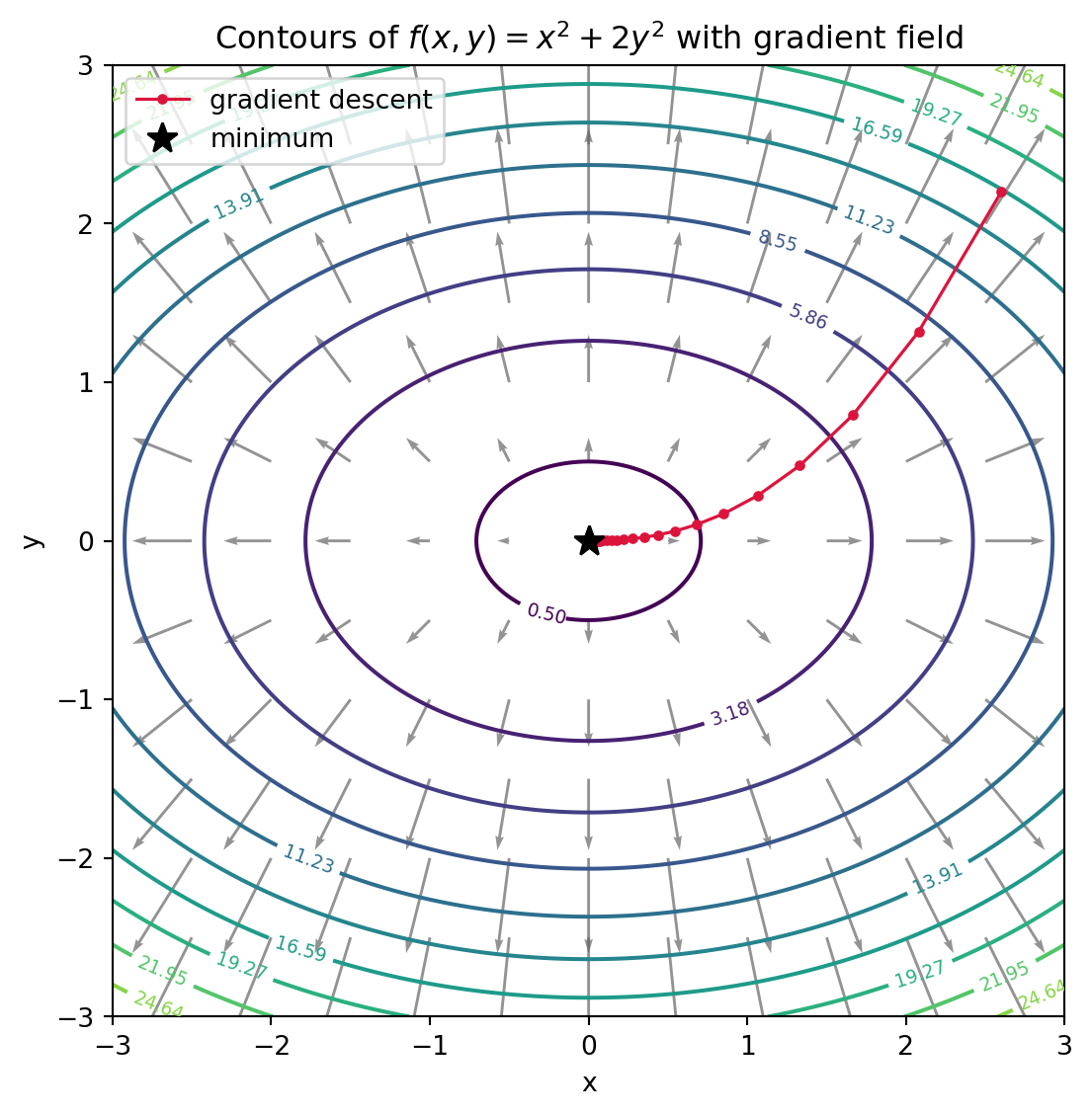
The plot below makes these ideas tangible. We take the bowl-shaped quadratic \(f(x, y) = x^2 + 2y^2\), whose gradient is \(\nabla f(x, y) = (2x,\; 4y)\). The contour lines are the level sets; the gray arrows form the gradient field, each pointing in the direction of steepest ascent and orthogonal to the contour it sits on; and the red path traces gradient descent stepping against the gradient toward the minimum at the origin. The cell also verifies the analytic gradient against a centered finite difference, so the math and the picture are checked against each other.
fn f(x:f64, y:f64) ->f64{ x * x +2.0* y * y}fn grad_f(x:f64, y:f64) -> [f64;2] { [2.0* x,4.0* y]}fn main() {// Gradient descent on the quadratic bowl.let eta =0.1;letmut point = [2.6_f64,2.2_f64];for _ in0..25{let g = grad_f(point[0], point[1]); point[0] -= eta * g[0]; point[1] -= eta * g[1];}// Verify the analytic gradient against a centered finite difference.let p = [1.3_f64,-0.7_f64];let eps =1e-6;let fd = [ (f(p[0] + eps, p[1]) - f(p[0] - eps, p[1])) / (2.0* eps), (f(p[0], p[1] + eps) - f(p[0], p[1] - eps)) / (2.0* eps), ];let analytic = grad_f(p[0], p[1]);println!("analytic gradient: {:?}", analytic);println!("finite difference: {:?}", fd);println!("descent endpoint : {:?}", point);}
27.5 5. The Jacobian Matrix for Vector-Valued Functions
27.5.1 5.1 From scalar outputs to vector outputs
So far \(f\) has produced a single scalar. Many functions in machine learning produce a vector instead. A neural network layer maps an input vector to an output vector; a softmax maps a vector of logits to a vector of probabilities. For such a function \(\mathbf{f}: \mathbb{R}^n \to \mathbb{R}^m\) with components
a single gradient vector no longer suffices. Each output component \(f_j\) has its own gradient, and we stack them into a matrix.
27.5.2 5.2 Definition of the Jacobian
The Jacobian matrix \(J\) of \(\mathbf{f}: \mathbb{R}^n \to \mathbb{R}^m\) is the \(m \times n\) matrix whose entry in row \(j\) and column \(i\) is the partial derivative of output \(j\) with respect to input \(i\):
Row \(j\) of the Jacobian is exactly the transpose of the gradient of \(f_j\). When \(m = 1\), the Jacobian is a single row, the gradient written horizontally. The Jacobian is thus the natural generalization of the gradient to vector-valued functions, and it provides the best local linear approximation of \(\mathbf{f}\):
The reason the Jacobian is indispensable for deep learning is the multivariable chain rule. A neural network is a composition of many functions, one per layer: \(\mathbf{f} = \mathbf{f}^{(L)} \circ \cdots \circ \mathbf{f}^{(2)} \circ \mathbf{f}^{(1)}\). The chain rule says the Jacobian of a composition is the product of the Jacobians of the pieces:
Because the final loss is a scalar, the overall Jacobian is a single row vector, the gradient of the loss with respect to the inputs. Backpropagation is precisely the algorithm that computes this product efficiently. Rather than forming each large Jacobian explicitly, it propagates a gradient vector backward through the network, multiplying by one layer Jacobian at a time. This is known as reverse-mode automatic differentiation, and it computes the gradient of a scalar loss with respect to all parameters at a cost comparable to a single forward pass, regardless of how many parameters there are. That efficiency is what makes training networks with billions of parameters feasible.
27.5.4 5.4 A concrete softmax Jacobian
The softmax function \(\mathbf{s}(\mathbf{z})\) with \(s_j = e^{z_j} / \sum_k e^{z_k}\) is a vector-to-vector map whose Jacobian appears in nearly every classification network. Its entries are
where \(\delta_{ji}\) is \(1\) when \(j = i\) and \(0\) otherwise. When this Jacobian is combined with the cross-entropy loss through the chain rule, the messy product collapses into the elegant expression \(\hat{y} - y\) encountered in Section 2.3, which is one reason the softmax and cross-entropy pairing is ubiquitous.
27.6 6. How Gradients Drive Gradient-Based Learning
27.6.1 6.1 The training loop
We can now assemble the full picture. Training a model is a loop with four steps. First, a forward pass computes the model output and the scalar loss \(L(\theta)\) on a batch of data. Second, backpropagation computes the gradient \(\nabla_\theta L\) by multiplying layer Jacobians in reverse. Third, an optimizer uses the gradient to update the parameters. Fourth, the loop repeats on a new batch. Every one of these steps is built on the partial derivatives, gradients, and Jacobians developed above.
27.6.2 6.2 Stochastic gradient descent
Computing the exact gradient over an entire dataset is expensive, so practitioners estimate it from a small random subset of examples called a mini-batch. The resulting algorithm, stochastic gradient descent, uses
where \(L_{\mathcal{B}_t}\) is the loss averaged over the current mini-batch \(\mathcal{B}_t\). The mini-batch gradient is a noisy but unbiased estimate of the full gradient. The noise is not purely a nuisance: it helps the optimizer escape shallow regions and contributes to the strong generalization observed in deep networks. Stochastic gradient descent is the workhorse that makes learning on massive datasets tractable.
27.6.3 6.3 Adaptive optimizers
Plain gradient descent uses one learning rate for all parameters. In practice the loss landscape is poorly scaled, with some directions far steeper than others, and a single global step size struggles. Momentum methods accumulate a running average of past gradients to smooth the trajectory and accelerate progress along consistent directions. Adaptive methods such as Adam maintain per-parameter estimates of both the mean and the variance of recent gradients, then scale each parameter update by its own factor. The update for parameter \(i\) is roughly
where \(\hat{m}_i\) is a bias-corrected estimate of the gradient mean and \(\hat{v}_i\) of its squared magnitude. Parameters with large, noisy gradients take smaller effective steps, while parameters with small, steady gradients take larger ones. These methods are still gradient descent at heart; they only reshape how the raw gradient is turned into a step.
27.6.4 6.4 When gradients misbehave
Because deep networks multiply many Jacobians together, the magnitude of the gradient can shrink toward zero or blow up toward infinity as it propagates through layers. These are the vanishing and exploding gradient problems. They explain a wide range of design choices in modern architectures: the use of the ReLU activation, whose derivative does not saturate to zero on the positive side; careful weight initialization that keeps the typical Jacobian close to norm preserving; normalization layers that stabilize the scale of activations; residual connections that provide a short, unobstructed path for gradients to flow backward; and gradient clipping, which caps the gradient norm to prevent destructive jumps. In every case the engineering goal is to keep the gradient informative, neither so small that learning stalls nor so large that it destabilizes. Seen this way, much of modern deep learning architecture is an effort to keep the chain of Jacobians well behaved so that gradient-based learning can do its work.
27.6.5 6.5 Summary
The gradient is the vector of partial derivatives that points in the direction of steepest ascent, with magnitude equal to the steepest rate of change. Its negative is the direction of fastest decrease, which is why gradient descent steps against the gradient. The directional derivative shows that the gradient encodes the rate of change in every direction at once, and the orthogonality to level sets gives steepest ascent its clean geometric picture. For vector-valued functions the Jacobian generalizes the gradient, and the chain rule expressed through Jacobian products is the mathematical content of backpropagation. Together these objects turn the abstract goal of minimizing a loss into a concrete, efficient, and scalable computation, which is why gradients sit at the foundation of essentially all modern machine learning.
27.7 References
Rumelhart, D. E., Hinton, G. E., and Williams, R. J. (1986). Learning representations by back-propagating errors. Nature, 323, 533 to 536. https://doi.org/10.1038/323533a0
Goodfellow, I., Bengio, Y., and Courville, A. (2016). Deep Learning. MIT Press. ISBN 9780262035613. https://www.deeplearningbook.org/
Deisenroth, M. P., Faisal, A. A., and Ong, C. S. (2020). Mathematics for Machine Learning. Cambridge University Press. https://doi.org/10.1017/9781108679930
Baydin, A. G., Pearlmutter, B. A., Radul, A. A., and Siskind, J. M. (2018). Automatic differentiation in machine learning: a survey. Journal of Machine Learning Research, 18(153), 1 to 43. https://jmlr.org/papers/v18/17-468.html
Kingma, D. P., and Ba, J. (2015). Adam: A method for stochastic optimization. International Conference on Learning Representations (ICLR). https://doi.org/10.48550/arXiv.1412.6980
Bottou, L., Curtis, F. E., and Nocedal, J. (2018). Optimization methods for large-scale machine learning. SIAM Review, 60(2), 223 to 311. https://doi.org/10.1137/16M1080173
Ruder, S. (2016). An overview of gradient descent optimization algorithms. arXiv preprint. https://doi.org/10.48550/arXiv.1609.04747
Nocedal, J., and Wright, S. J. (2006). Numerical Optimization, 2nd ed. Springer. https://doi.org/10.1007/978-0-387-40065-5
Source Code
# Gradients and Partial DerivativesModern machine learning rests on a deceptively simple idea: to improve a model, measure how a small change in each parameter changes a loss, then nudge every parameter in the direction that reduces that loss the most. The mathematical object that packages all of those per-parameter sensitivities into a single quantity is the gradient. Understanding gradients, the partial derivatives they are built from, and the geometric meaning of steepest ascent is the conceptual core of gradient-based learning. This chapter develops that machinery from the ground up and connects each step to the practice of training neural networks.## 1. From Single-Variable Derivatives to Partial Derivatives### 1.1 The derivative as a rate of changeFor a function of one variable $f: \mathbb{R} \to \mathbb{R}$, the derivative at a point $x$ measures the instantaneous rate of change of the output with respect to the input:$$f'(x) = \lim_{h \to 0} \frac{f(x + h) - f(x)}{h}.$$Geometrically, $f'(x)$ is the slope of the line tangent to the graph of $f$ at $x$. If $f'(x) > 0$, increasing $x$ increases $f$; if $f'(x) < 0$, increasing $x$ decreases $f$. This sign information is exactly what an optimizer needs: to make $f$ smaller, move $x$ opposite to the sign of the derivative.Machine learning loss functions, however, almost never depend on a single variable. A small neural network already has thousands of parameters, and large language models have hundreds of billions. We therefore need a notion of derivative for functions that accept many inputs at once.### 1.2 Partial derivativesLet $f: \mathbb{R}^n \to \mathbb{R}$ be a scalar-valued function of $n$ variables, written $f(x_1, x_2, \ldots, x_n)$. The partial derivative of $f$ with respect to $x_i$ measures how $f$ changes when we vary $x_i$ alone, holding every other variable fixed:$$\frac{\partial f}{\partial x_i} = \lim_{h \to 0} \frac{f(x_1, \ldots, x_i + h, \ldots, x_n) - f(x_1, \ldots, x_i, \ldots, x_n)}{h}.$$The mechanics are identical to ordinary differentiation: treat all variables except $x_i$ as constants, then differentiate normally. Consider$$f(x, y) = x^2 y + \sin(y).$$Holding $y$ constant and differentiating with respect to $x$ gives $\frac{\partial f}{\partial x} = 2xy$. Holding $x$ constant and differentiating with respect to $y$ gives $\frac{\partial f}{\partial y} = x^2 + \cos(y)$. Each partial derivative is itself a function of all the variables, so it can be evaluated at any point in the domain.### 1.3 Why partial derivatives matter for learningIn supervised learning we define a loss $L(\theta)$ that depends on a parameter vector $\theta = (\theta_1, \ldots, \theta_n)$. The partial derivative $\frac{\partial L}{\partial \theta_i}$ answers a precise question: if I increase parameter $\theta_i$ by a tiny amount and leave the rest untouched, does the loss go up or down, and how fast? Every parameter in a model gets its own such answer. Collecting all of these answers into one structure is what produces the gradient, the central object of this chapter.## 2. The Gradient Vector### 2.1 DefinitionThe gradient of a scalar function $f: \mathbb{R}^n \to \mathbb{R}$ is the vector of all its first-order partial derivatives:$$\nabla f(\mathbf{x}) = \left( \frac{\partial f}{\partial x_1}, \frac{\partial f}{\partial x_2}, \ldots, \frac{\partial f}{\partial x_n} \right).$$The symbol $\nabla$ is called nabla or del. The gradient is a vector field: at every point $\mathbf{x}$ in the domain it returns a vector in $\mathbb{R}^n$, the same dimension as the input space. For the example $f(x, y) = x^2 y + \sin(y)$ above,$$\nabla f(x, y) = \left( 2xy, \; x^2 + \cos(y) \right).$$At the point $(1, 0)$ this evaluates to $\nabla f(1, 0) = (0, 2)$. Every symbol here has a fixed meaning that is worth stating explicitly: $\mathbf{x} = (x_1, \ldots, x_n)$ is the input point, $n$ is the dimension of the input space, $\frac{\partial f}{\partial x_i}$ is the partial derivative defined in Section 1.2, and $\nabla f(\mathbf{x})$ is an $n$ dimensional vector that lives in the same space as $\mathbf{x}$.### 2.2 The gradient and the linear approximationThe deepest reason the gradient is useful comes from the first-order Taylor expansion. Near a point $\mathbf{x}$, a differentiable function is well approximated by a linear function, and the gradient supplies its coefficients:$$f(\mathbf{x} + \mathbf{v}) \approx f(\mathbf{x}) + \nabla f(\mathbf{x}) \cdot \mathbf{v},$$where $\nabla f(\mathbf{x}) \cdot \mathbf{v}$ is the dot product. This says that the change in $f$ caused by a small displacement $\mathbf{v}$ is, to first order, the dot product of the gradient with that displacement. The entire theory of gradient-based optimization is an exploitation of this single approximation. If we want to decrease $f$, we should choose a displacement $\mathbf{v}$ that makes the dot product $\nabla f(\mathbf{x}) \cdot \mathbf{v}$ as negative as possible.### 2.3 Gradients of common machine learning lossesTwo gradients appear so often that they are worth committing to memory. For linear regression with prediction $\hat{y} = \mathbf{w} \cdot \mathbf{x}$ and squared error loss $L = \frac{1}{2}(\hat{y} - y)^2$, the gradient with respect to the weights is$$\nabla_{\mathbf{w}} L = (\hat{y} - y)\,\mathbf{x}.$$The gradient is the prediction error scaled by the input. For logistic regression with sigmoid output $\hat{y} = \sigma(\mathbf{w} \cdot \mathbf{x})$ and cross-entropy loss, the gradient takes the same clean form, $(\hat{y} - y)\,\mathbf{x}$. This is not a coincidence; it reflects a structural relationship between these loss functions and their matched output activations, and it is one reason cross-entropy is the default loss for classification.## 3. Directional Derivatives### 3.1 Generalizing the partial derivativeA partial derivative measures change along one coordinate axis. But we might want to know how $f$ changes as we move in an arbitrary direction, not just along an axis. The directional derivative captures this. Given a unit vector $\mathbf{u}$ (so that $\|\mathbf{u}\| = 1$), the directional derivative of $f$ at $\mathbf{x}$ in the direction $\mathbf{u}$ is$$D_{\mathbf{u}} f(\mathbf{x}) = \lim_{h \to 0} \frac{f(\mathbf{x} + h\,\mathbf{u}) - f(\mathbf{x})}{h}.$$When $\mathbf{u}$ is a coordinate axis vector such as $(1, 0, \ldots, 0)$, the directional derivative reduces to the corresponding partial derivative. The directional derivative therefore generalizes the partial derivative to every possible direction of travel.### 3.2 The gradient computes every directional derivativeA central theorem of multivariable calculus states that for a differentiable function, the directional derivative is the dot product of the gradient with the direction:$$D_{\mathbf{u}} f(\mathbf{x}) = \nabla f(\mathbf{x}) \cdot \mathbf{u}.$$This is a remarkable economy. We do not need a separate limit for every direction. Once we know the gradient, a single dot product produces the rate of change along any direction we like. The gradient thus encodes the complete local first-order behavior of the function in one vector of $n$ numbers.A short proof makes the identity concrete. Define the single-variable function $g(h) = f(\mathbf{x} + h\,\mathbf{u})$, which traces the value of $f$ along the ray through $\mathbf{x}$ in direction $\mathbf{u}$. By definition $D_{\mathbf{u}} f(\mathbf{x}) = g'(0)$. Writing the $i$-th coordinate of $\mathbf{x} + h\,\mathbf{u}$ as $x_i + h\,u_i$ and applying the multivariable chain rule,$$g'(h) = \sum_{i=1}^{n} \frac{\partial f}{\partial x_i}(\mathbf{x} + h\,\mathbf{u}) \cdot \frac{d(x_i + h\,u_i)}{dh} = \sum_{i=1}^{n} \frac{\partial f}{\partial x_i}(\mathbf{x} + h\,\mathbf{u}) \, u_i.$$Evaluating at $h = 0$ gives $g'(0) = \sum_{i=1}^{n} \frac{\partial f}{\partial x_i}(\mathbf{x})\, u_i = \nabla f(\mathbf{x}) \cdot \mathbf{u}$, which is the claimed identity.### 3.3 A worked exampleTake $f(x, y) = x^2 y + \sin(y)$ from above, with gradient $\nabla f(x, y) = (2xy,\; x^2 + \cos y)$. At the point $\mathbf{x} = (1, 0)$ the gradient is $\nabla f(1, 0) = (0, 2)$. Suppose we want the rate of change in the direction of the vector $(3, 4)$. We first normalize it to unit length: $\|(3,4)\| = 5$, so $\mathbf{u} = (3/5,\; 4/5)$. The directional derivative is then$$D_{\mathbf{u}} f(1, 0) = \nabla f(1,0) \cdot \mathbf{u} = (0)(\tfrac{3}{5}) + (2)(\tfrac{4}{5}) = \tfrac{8}{5} = 1.6.$$Moving from $(1,0)$ a tiny step along $(3/5,\,4/5)$ increases $f$ at a rate of $1.6$ per unit of distance traveled. By the steepest-ascent result of the next section, the largest possible rate at this point is $\|\nabla f(1,0)\| = \|(0,2)\| = 2$, achieved by moving in the direction $(0, 1)$, and indeed $1.6 < 2$ as it must be.## 4. The Gradient as the Direction of Steepest Ascent### 4.1 The steepest ascent propertyWe can now answer the question that motivates optimization: in which direction does $f$ increase fastest? Using the dot product form of the directional derivative and the geometric identity $\mathbf{a} \cdot \mathbf{b} = \|\mathbf{a}\| \, \|\mathbf{b}\| \cos\phi$, where $\phi$ is the angle between the vectors, we have$$D_{\mathbf{u}} f(\mathbf{x}) = \nabla f(\mathbf{x}) \cdot \mathbf{u} = \|\nabla f(\mathbf{x})\| \, \|\mathbf{u}\| \cos\phi = \|\nabla f(\mathbf{x})\| \cos\phi,$$since $\mathbf{u}$ is a unit vector. The directional derivative is largest when $\cos\phi = 1$, that is when $\phi = 0$ and $\mathbf{u}$ points in the same direction as $\nabla f(\mathbf{x})$. We conclude:The gradient $\nabla f(\mathbf{x})$ points in the direction of steepest ascent, and its magnitude $\|\nabla f(\mathbf{x})\|$ equals the maximum rate of increase of $f$ at that point.By the same argument, $\cos\phi = -1$ gives the most negative directional derivative, so the direction of steepest descent is $-\nabla f(\mathbf{x})$. This is the single most important fact behind gradient descent: to reduce a loss as quickly as possible, step in the direction opposite the gradient.### 4.2 The gradient is orthogonal to level setsA level set of $f$ is the set of points where $f$ takes a constant value, written $\{ \mathbf{x} : f(\mathbf{x}) = c \}$. In two dimensions these are the contour lines on a topographic map. If we move along a level set, $f$ does not change, so the directional derivative along the level set is zero. But $D_{\mathbf{u}} f = \nabla f \cdot \mathbf{u} = 0$ means the gradient is perpendicular to that direction. Therefore the gradient is always orthogonal to the level set passing through a point. Steepest ascent is achieved by leaving the contour at a right angle, which matches the intuition that the quickest way uphill is to walk perpendicular to the lines of constant elevation.### 4.3 Gradient descentThese facts crystallize into the gradient descent update rule. Starting from an initial parameter vector $\theta_0$, we iterate$$\theta_{t+1} = \theta_t - \eta \, \nabla L(\theta_t),$$where $\eta > 0$ is the learning rate, a small positive step size. Each step moves the parameters a short distance in the direction of steepest descent of the loss. The first-order Taylor approximation guarantees that for a sufficiently small $\eta$, the loss decreases at every step until a point where the gradient vanishes. A point where $\nabla L(\theta) = \mathbf{0}$ is called a stationary point; it may be a local minimum, a local maximum, or a saddle point, and distinguishing among these requires second-order information that we set aside here.The learning rate governs the tension at the heart of training. If $\eta$ is too small, progress is slow and many iterations are needed. If $\eta$ is too large, the linear approximation that justifies the step breaks down, and the loss can oscillate or diverge. Choosing and adapting $\eta$ is one of the central practical concerns of training, and it motivates the adaptive optimizers discussed below.### 4.4 Visualizing the gradient field and descentThe plot below makes these ideas tangible. We take the bowl-shaped quadratic $f(x, y) = x^2 + 2y^2$, whose gradient is $\nabla f(x, y) = (2x,\; 4y)$. The contour lines are the level sets; the gray arrows form the gradient field, each pointing in the direction of steepest ascent and orthogonal to the contour it sits on; and the red path traces gradient descent stepping against the gradient toward the minimum at the origin. The cell also verifies the analytic gradient against a centered finite difference, so the math and the picture are checked against each other.::: {.panel-tabset}## Python```{python}#| label: fig-gradient-field#| fig-cap: "Gradient field and a descent path on a quadratic bowl."import numpy as npimport matplotlib.pyplot as pltrng = np.random.default_rng(0)def f(x, y):return x**2+2.0* y**2def grad_f(x, y):return np.array([2.0* x, 4.0* y])xs = np.linspace(-3.0, 3.0, 400)ys = np.linspace(-3.0, 3.0, 400)X, Y = np.meshgrid(xs, ys)Z = f(X, Y)xg = np.linspace(-3.0, 3.0, 13)yg = np.linspace(-3.0, 3.0, 13)XG, YG = np.meshgrid(xg, yg)U, V =2.0* XG, 4.0* YGeta =0.1point = np.array([2.6, 2.2])path = [point.copy()]for _ inrange(25): point = point - eta * grad_f(point[0], point[1]) path.append(point.copy())path = np.array(path)fig, ax = plt.subplots(figsize=(7, 6))cs = ax.contour(X, Y, Z, levels=np.linspace(0.5, 30, 12), cmap="viridis")ax.clabel(cs, inline=True, fontsize=7)ax.quiver(XG, YG, U, V, color="0.4", alpha=0.7, scale=80, width=0.003)ax.plot(path[:, 0], path[:, 1], "o-", color="crimson", markersize=3, linewidth=1.2, label="gradient descent")ax.plot(0, 0, "k*", markersize=12, label="minimum")ax.set_xlabel("x")ax.set_ylabel("y")ax.set_title(r"Contours of $f(x,y)=x^2+2y^2$ with gradient field")ax.legend(loc="upper left")ax.set_aspect("equal")fig.tight_layout()# Verify the analytic gradient against a centered finite difference.p = np.array([1.3, -0.7])eps =1e-6fd = np.array([ (f(p[0] + eps, p[1]) - f(p[0] - eps, p[1])) / (2* eps), (f(p[0], p[1] + eps) - f(p[0], p[1] - eps)) / (2* eps),])print("analytic gradient:", np.round(grad_f(p[0], p[1]), 6))print("finite difference:", np.round(fd, 6))print("descent endpoint :", np.round(path[-1], 6))plt.show()```## Julia```juliausingLinearAlgebraf(x, y) = x^2+2.0* y^2grad_f(x, y) = [2.0* x, 4.0* y]# Gradient descent on the quadratic bowl.eta =0.1point = [2.6, 2.2]path = [copy(point)]for _ in1:25global point = point .- eta .*grad_f(point[1], point[2])push!(path, copy(point))end# Verify the analytic gradient against a centered finite difference.p = [1.3, -0.7]eps =1e-6fd = [ (f(p[1] + eps, p[2]) -f(p[1] - eps, p[2])) / (2eps), (f(p[1], p[2] + eps) -f(p[1], p[2] - eps)) / (2eps),]println("analytic gradient: ", grad_f(p[1], p[2]))println("finite difference: ", round.(fd, digits=6))println("descent endpoint : ", round.(path[end], digits=6))```## Rust```rustfn f(x: f64, y: f64) -> f64 { x * x +2.0* y * y}fn grad_f(x: f64, y: f64) -> [f64; 2] { [2.0* x, 4.0* y]}fn main() {// Gradient descent on the quadratic bowl. let eta =0.1; let mut point = [2.6_f64, 2.2_f64];for _ in0..25 { let g =grad_f(point[0], point[1]); point[0] -= eta * g[0]; point[1] -= eta * g[1]; }// Verify the analytic gradient against a centered finite difference. let p = [1.3_f64, -0.7_f64]; let eps =1e-6; let fd = [ (f(p[0] + eps, p[1]) -f(p[0] - eps, p[1])) / (2.0* eps), (f(p[0], p[1] + eps) -f(p[0], p[1] - eps)) / (2.0* eps), ]; let analytic =grad_f(p[0], p[1]); println!("analytic gradient: {:?}", analytic); println!("finite difference: {:?}", fd); println!("descent endpoint : {:?}", point);}```:::## 5. The Jacobian Matrix for Vector-Valued Functions### 5.1 From scalar outputs to vector outputsSo far $f$ has produced a single scalar. Many functions in machine learning produce a vector instead. A neural network layer maps an input vector to an output vector; a softmax maps a vector of logits to a vector of probabilities. For such a function $\mathbf{f}: \mathbb{R}^n \to \mathbb{R}^m$ with components$$\mathbf{f}(\mathbf{x}) = \big( f_1(\mathbf{x}), f_2(\mathbf{x}), \ldots, f_m(\mathbf{x}) \big),$$a single gradient vector no longer suffices. Each output component $f_j$ has its own gradient, and we stack them into a matrix.### 5.2 Definition of the JacobianThe Jacobian matrix $J$ of $\mathbf{f}: \mathbb{R}^n \to \mathbb{R}^m$ is the $m \times n$ matrix whose entry in row $j$ and column $i$ is the partial derivative of output $j$ with respect to input $i$:$$J_{ji} = \frac{\partial f_j}{\partial x_i}, \qquadJ = \begin{bmatrix}\dfrac{\partial f_1}{\partial x_1} & \cdots & \dfrac{\partial f_1}{\partial x_n} \\\vdots & \ddots & \vdots \\\dfrac{\partial f_m}{\partial x_1} & \cdots & \dfrac{\partial f_m}{\partial x_n}\end{bmatrix}.$$Row $j$ of the Jacobian is exactly the transpose of the gradient of $f_j$. When $m = 1$, the Jacobian is a single row, the gradient written horizontally. The Jacobian is thus the natural generalization of the gradient to vector-valued functions, and it provides the best local linear approximation of $\mathbf{f}$:$$\mathbf{f}(\mathbf{x} + \mathbf{v}) \approx \mathbf{f}(\mathbf{x}) + J(\mathbf{x})\,\mathbf{v}.$$### 5.3 The chain rule and backpropagationThe reason the Jacobian is indispensable for deep learning is the multivariable chain rule. A neural network is a composition of many functions, one per layer: $\mathbf{f} = \mathbf{f}^{(L)} \circ \cdots \circ \mathbf{f}^{(2)} \circ \mathbf{f}^{(1)}$. The chain rule says the Jacobian of a composition is the product of the Jacobians of the pieces:$$J_{\mathbf{f}} = J_{\mathbf{f}^{(L)}} \, J_{\mathbf{f}^{(L-1)}} \cdots J_{\mathbf{f}^{(1)}}.$$Because the final loss is a scalar, the overall Jacobian is a single row vector, the gradient of the loss with respect to the inputs. Backpropagation is precisely the algorithm that computes this product efficiently. Rather than forming each large Jacobian explicitly, it propagates a gradient vector backward through the network, multiplying by one layer Jacobian at a time. This is known as reverse-mode automatic differentiation, and it computes the gradient of a scalar loss with respect to all parameters at a cost comparable to a single forward pass, regardless of how many parameters there are. That efficiency is what makes training networks with billions of parameters feasible.### 5.4 A concrete softmax JacobianThe softmax function $\mathbf{s}(\mathbf{z})$ with $s_j = e^{z_j} / \sum_k e^{z_k}$ is a vector-to-vector map whose Jacobian appears in nearly every classification network. Its entries are$$\frac{\partial s_j}{\partial z_i} = s_j (\delta_{ji} - s_i),$$where $\delta_{ji}$ is $1$ when $j = i$ and $0$ otherwise. When this Jacobian is combined with the cross-entropy loss through the chain rule, the messy product collapses into the elegant expression $\hat{y} - y$ encountered in Section 2.3, which is one reason the softmax and cross-entropy pairing is ubiquitous.## 6. How Gradients Drive Gradient-Based Learning### 6.1 The training loopWe can now assemble the full picture. Training a model is a loop with four steps. First, a forward pass computes the model output and the scalar loss $L(\theta)$ on a batch of data. Second, backpropagation computes the gradient $\nabla_\theta L$ by multiplying layer Jacobians in reverse. Third, an optimizer uses the gradient to update the parameters. Fourth, the loop repeats on a new batch. Every one of these steps is built on the partial derivatives, gradients, and Jacobians developed above.### 6.2 Stochastic gradient descentComputing the exact gradient over an entire dataset is expensive, so practitioners estimate it from a small random subset of examples called a mini-batch. The resulting algorithm, stochastic gradient descent, uses$$\theta_{t+1} = \theta_t - \eta \, \nabla_\theta L_{\mathcal{B}_t}(\theta_t),$$where $L_{\mathcal{B}_t}$ is the loss averaged over the current mini-batch $\mathcal{B}_t$. The mini-batch gradient is a noisy but unbiased estimate of the full gradient. The noise is not purely a nuisance: it helps the optimizer escape shallow regions and contributes to the strong generalization observed in deep networks. Stochastic gradient descent is the workhorse that makes learning on massive datasets tractable.### 6.3 Adaptive optimizersPlain gradient descent uses one learning rate for all parameters. In practice the loss landscape is poorly scaled, with some directions far steeper than others, and a single global step size struggles. Momentum methods accumulate a running average of past gradients to smooth the trajectory and accelerate progress along consistent directions. Adaptive methods such as Adam maintain per-parameter estimates of both the mean and the variance of recent gradients, then scale each parameter update by its own factor. The update for parameter $i$ is roughly$$\theta_i \leftarrow \theta_i - \eta \, \frac{\hat{m}_i}{\sqrt{\hat{v}_i} + \epsilon},$$where $\hat{m}_i$ is a bias-corrected estimate of the gradient mean and $\hat{v}_i$ of its squared magnitude. Parameters with large, noisy gradients take smaller effective steps, while parameters with small, steady gradients take larger ones. These methods are still gradient descent at heart; they only reshape how the raw gradient is turned into a step.### 6.4 When gradients misbehaveBecause deep networks multiply many Jacobians together, the magnitude of the gradient can shrink toward zero or blow up toward infinity as it propagates through layers. These are the vanishing and exploding gradient problems. They explain a wide range of design choices in modern architectures: the use of the ReLU activation, whose derivative does not saturate to zero on the positive side; careful weight initialization that keeps the typical Jacobian close to norm preserving; normalization layers that stabilize the scale of activations; residual connections that provide a short, unobstructed path for gradients to flow backward; and gradient clipping, which caps the gradient norm to prevent destructive jumps. In every case the engineering goal is to keep the gradient informative, neither so small that learning stalls nor so large that it destabilizes. Seen this way, much of modern deep learning architecture is an effort to keep the chain of Jacobians well behaved so that gradient-based learning can do its work.### 6.5 SummaryThe gradient is the vector of partial derivatives that points in the direction of steepest ascent, with magnitude equal to the steepest rate of change. Its negative is the direction of fastest decrease, which is why gradient descent steps against the gradient. The directional derivative shows that the gradient encodes the rate of change in every direction at once, and the orthogonality to level sets gives steepest ascent its clean geometric picture. For vector-valued functions the Jacobian generalizes the gradient, and the chain rule expressed through Jacobian products is the mathematical content of backpropagation. Together these objects turn the abstract goal of minimizing a loss into a concrete, efficient, and scalable computation, which is why gradients sit at the foundation of essentially all modern machine learning.## References1. Rumelhart, D. E., Hinton, G. E., and Williams, R. J. (1986). Learning representations by back-propagating errors. *Nature*, 323, 533 to 536. https://doi.org/10.1038/323533a02. Goodfellow, I., Bengio, Y., and Courville, A. (2016). *Deep Learning*. MIT Press. ISBN 9780262035613. https://www.deeplearningbook.org/3. Deisenroth, M. P., Faisal, A. A., and Ong, C. S. (2020). *Mathematics for Machine Learning*. Cambridge University Press. https://doi.org/10.1017/97811086799304. Baydin, A. G., Pearlmutter, B. A., Radul, A. A., and Siskind, J. M. (2018). Automatic differentiation in machine learning: a survey. *Journal of Machine Learning Research*, 18(153), 1 to 43. https://jmlr.org/papers/v18/17-468.html5. Kingma, D. P., and Ba, J. (2015). Adam: A method for stochastic optimization. *International Conference on Learning Representations (ICLR)*. https://doi.org/10.48550/arXiv.1412.69806. Bottou, L., Curtis, F. E., and Nocedal, J. (2018). Optimization methods for large-scale machine learning. *SIAM Review*, 60(2), 223 to 311. https://doi.org/10.1137/16M10801737. Ruder, S. (2016). An overview of gradient descent optimization algorithms. *arXiv preprint*. https://doi.org/10.48550/arXiv.1609.047478. Nocedal, J., and Wright, S. J. (2006). *Numerical Optimization*, 2nd ed. Springer. https://doi.org/10.1007/978-0-387-40065-5