Ordinary least squares is the workhorse of linear modeling, but it has a well known failure mode. When predictors are numerous, correlated, or nearly collinear, the least squares estimator becomes unstable: small perturbations in the data produce wildly different coefficient vectors, and predictions on new data degrade. Ridge regression, introduced by Hoerl and Kennard in 1970, addresses this by adding a quadratic penalty on the coefficient magnitudes. The result is a biased estimator that trades a small amount of bias for a large reduction in variance, and that remains well defined even when the design matrix is rank deficient. This chapter develops ridge regression from five complementary angles: the penalized objective, the closed form solution, the bias variance decomposition, the Bayesian interpretation as a Gaussian prior, and the shrinkage view through the singular value decomposition.
89.1 1. The Penalized Objective
89.1.1 1.1 Setup and notation
Let \(\mathbf{X} \in \mathbb{R}^{n \times p}\) denote the design matrix with \(n\) observations and \(p\) predictors, and let \(\mathbf{y} \in \mathbb{R}^{n}\) denote the response vector. We seek a coefficient vector \(\boldsymbol{\beta} \in \mathbb{R}^{p}\). Ordinary least squares (OLS) minimizes the residual sum of squares,
The OLS solution requires \(\mathbf{X}^{\top}\mathbf{X}\) to be invertible. When \(p > n\), or when columns of \(\mathbf{X}\) are linearly dependent, this matrix is singular and the solution is not unique. Even when it is technically invertible, near collinearity makes \(\mathbf{X}^{\top}\mathbf{X}\) ill conditioned, so the inverse amplifies noise.
89.1.2 1.2 Adding the L2 penalty
Ridge regression augments the objective with a penalty proportional to the squared Euclidean norm of the coefficients:
where \(\lambda \geq 0\) is the regularization strength. The term \(\lambda \lVert \boldsymbol{\beta} \rVert_2^2 = \lambda \sum_{j=1}^{p} \beta_j^2\) discourages large coefficients. At \(\lambda = 0\) we recover OLS. As \(\lambda \to \infty\) the penalty dominates and every coefficient is driven toward zero.
An equivalent formulation states ridge as a constrained problem,
with a one to one correspondence between \(\lambda\) and the budget \(t\). This geometric picture shows that ridge confines the solution to a Euclidean ball, and the smooth spherical boundary is why ridge shrinks coefficients continuously rather than setting them exactly to zero, in contrast to the L1 penalty of the lasso.
89.1.3 1.3 The intercept and standardization
The penalty should not apply to the intercept, since shrinking the intercept would make the fit depend on the arbitrary origin of the response. In practice we center \(\mathbf{y}\) and each column of \(\mathbf{X}\), fit a ridge model without an intercept on the centered data, and recover the intercept as \(\hat{\beta}_0 = \bar{y}\) on the original scale. Furthermore, because the penalty \(\sum_j \beta_j^2\) treats every coefficient equally, the solution is not invariant to the units of each predictor. A variable measured in millimeters receives a different penalty than the same variable in meters. The standard remedy is to standardize each predictor to unit variance before fitting, so that the penalty is applied on a common scale. These two preprocessing steps, centering and scaling, are essential for ridge to behave as intended.
89.2 2. The Closed Form Solution
89.2.1 2.1 Deriving the normal equations
The ridge objective is a smooth convex quadratic in \(\boldsymbol{\beta}\), so we find its minimizer by setting the gradient to zero. Write the objective as
The matrix \(\mathbf{X}^{\top}\mathbf{X}\) is symmetric positive semidefinite, so its eigenvalues are nonnegative. Adding \(\lambda \mathbf{I}_p\) for any \(\lambda > 0\) shifts every eigenvalue up by \(\lambda\), making the eigenvalues strictly positive. The matrix \(\mathbf{X}^{\top}\mathbf{X} + \lambda \mathbf{I}_p\) is therefore positive definite and invertible regardless of the rank of \(\mathbf{X}\). This is the algebraic heart of ridge regularization. Even in the \(p > n\) regime, where \(\mathbf{X}^{\top}\mathbf{X}\) is singular, the ridge estimator is unique and stable. The penalty also improves the condition number: if \(\mathbf{X}^{\top}\mathbf{X}\) has eigenvalues \(d_j^2\), then the condition number drops from \(d_{\max}^2 / d_{\min}^2\) to \((d_{\max}^2 + \lambda)/(d_{\min}^2 + \lambda)\), which is much closer to one when \(\lambda\) is comparable to the smaller eigenvalues.
89.2.3 2.3 Computational notes
Two practical formulations matter. When \(p \leq n\), solving the \(p \times p\) system above is efficient. When \(p \gg n\), the Woodbury identity gives an equivalent expression that inverts an \(n \times n\) matrix instead,
which is cheaper in the high dimensional setting and exposes the kernel structure that underlies kernel ridge regression. In code, one should never form an explicit inverse; instead solve the linear system directly with a Cholesky factorization, since \(\mathbf{X}^{\top}\mathbf{X} + \lambda \mathbf{I}\) is positive definite. Section 6 gives a runnable implementation.
89.3 3. The Bias Variance Effect
89.3.1 3.1 The decomposition
For a fixed test input \(\mathbf{x}_0\), the expected squared prediction error decomposes into three parts: the irreducible noise variance, the squared bias of the estimator, and its variance. Ridge regression deliberately moves along this tradeoff. OLS is unbiased but can have enormous variance under collinearity. Ridge introduces bias by shrinking coefficients toward zero, but the variance reduction more than compensates over a useful range of \(\lambda\), lowering the total expected error.
89.3.2 3.2 Bias and variance of the ridge estimator
Assume the linear model \(\mathbf{y} = \mathbf{X}\boldsymbol{\beta}^{\star} + \boldsymbol{\varepsilon}\) with \(\mathbb{E}[\boldsymbol{\varepsilon}] = \mathbf{0}\) and \(\operatorname{Cov}(\boldsymbol{\varepsilon}) = \sigma^2 \mathbf{I}\). Let \(\mathbf{Z}_\lambda = (\mathbf{X}^{\top}\mathbf{X} + \lambda \mathbf{I})^{-1}\mathbf{X}^{\top}\), so that \(\hat{\boldsymbol{\beta}}^{\text{ridge}} = \mathbf{Z}_\lambda \mathbf{y}\). Taking expectations,
Each factor of \((\mathbf{X}^{\top}\mathbf{X} + \lambda \mathbf{I})^{-1}\) shrinks as \(\lambda\) grows, so the variance decreases monotonically in \(\lambda\). Bias increases while variance decreases, and the mean squared error is minimized at some intermediate \(\lambda\).
89.3.3 3.3 The existence theorem
A central theoretical result, due to Hoerl and Kennard, is that there always exists a \(\lambda > 0\) for which the ridge estimator has strictly smaller total mean squared error than OLS. In other words, OLS is never the optimal point on the bias variance curve. The catch is that the optimal \(\lambda\) depends on the unknown true coefficients and noise level, so in practice it must be chosen from data, most commonly by \(k\) fold cross validation or by generalized cross validation, which has an efficient leave one out form for ridge.
89.4 4. The Bayesian Interpretation
89.4.1 4.1 Gaussian likelihood and Gaussian prior
Ridge regression has a clean probabilistic reading as the maximum a posteriori (MAP) estimate under a Gaussian likelihood and a Gaussian prior on the coefficients. Suppose the data are generated as
Maximizing the posterior is equivalent to minimizing the negative log posterior. Multiplying by \(2\sigma^2\) leaves the minimizer unchanged and yields exactly the ridge objective,
The regularization parameter is therefore \(\lambda = \sigma^2 / \tau^2\). A strong prior belief in small coefficients (small \(\tau^2\)) corresponds to large \(\lambda\), while a diffuse prior (large \(\tau^2\)) corresponds to small \(\lambda\), recovering OLS in the limit \(\tau^2 \to \infty\).
89.4.3 4.3 Beyond the point estimate
Because both the prior and the likelihood are Gaussian, the full posterior is itself Gaussian, with mean equal to the ridge estimate and covariance \((\sigma^{-2}\mathbf{X}^{\top}\mathbf{X} + \tau^{-2}\mathbf{I})^{-1}\). This is more than a curiosity. It means ridge is the posterior mean of a conjugate Bayesian linear model, so it delivers calibrated uncertainty intervals for free, and it connects directly to Gaussian process regression, where the same Gaussian prior is placed in a feature space. The Bayesian view also reframes the choice of \(\lambda\) as a question of prior variance, which can be estimated by maximizing the marginal likelihood, an approach known as empirical Bayes or evidence maximization.
89.5 5. The Shrinkage and SVD View
89.5.1 5.1 Singular value decomposition of the design
The most illuminating analysis of ridge comes from the singular value decomposition (SVD) of the design matrix. Write
where \(\mathbf{U} \in \mathbb{R}^{n \times p}\) and \(\mathbf{V} \in \mathbb{R}^{p \times p}\) have orthonormal columns and \(\mathbf{D} = \operatorname{diag}(d_1, \ldots, d_p)\) holds the singular values \(d_1 \geq d_2 \geq \cdots \geq d_p \geq 0\). The columns of \(\mathbf{V}\) are the principal directions of the predictor space, and \(d_j^2\) measures the variance of the data along direction \(\mathbf{v}_j\).
89.5.2 5.2 Ridge fitted values as filtered components
To derive the shrinkage form, substitute \(\mathbf{X} = \mathbf{U}\mathbf{D}\mathbf{V}^{\top}\) into the closed form solution. Using the orthonormality \(\mathbf{V}^{\top}\mathbf{V} = \mathbf{I}\), the penalized Gram matrix becomes
whose inverse is \(\mathbf{V}(\mathbf{D}^2 + \lambda \mathbf{I})^{-1}\mathbf{V}^{\top}\) because \(\mathbf{D}^2 + \lambda \mathbf{I}\) is diagonal. The coefficient vector is then
Left multiplying by \(\mathbf{X} = \mathbf{U}\mathbf{D}\mathbf{V}^{\top}\) and again using \(\mathbf{V}^{\top}\mathbf{V} = \mathbf{I}\), the diagonal term \(d_j \cdot d_j/(d_j^2 + \lambda)\) collects into the shrinkage factor, so the ridge fitted values are
The factor \(f_j\) reveals exactly how ridge acts. Directions with large singular values, where \(d_j^2 \gg \lambda\), have \(f_j \approx 1\) and are barely shrunk. Directions with small singular values, where \(d_j^2 \ll \lambda\), have \(f_j \approx d_j^2 / \lambda \approx 0\) and are shrunk heavily. Because \(d_j^2\) is the variance of the data along \(\mathbf{v}_j\), ridge preserves high variance directions and suppresses low variance directions. This is precisely where it helps: low variance directions are the ones along which collinearity makes the OLS coefficients explode, because dividing the projected response by a tiny \(d_j\) amplifies noise. Ridge tempers that division by adding \(\lambda\) to the denominator, so unstable directions are damped rather than amplified.
89.5.4 5.4 Effective degrees of freedom
The shrinkage factors also give ridge a natural complexity measure. The hat matrix for ridge is \(\mathbf{H}_\lambda = \mathbf{X}(\mathbf{X}^{\top}\mathbf{X} + \lambda \mathbf{I})^{-1}\mathbf{X}^{\top}\), and its trace is
This effective degrees of freedom decreases smoothly from \(p\) at \(\lambda = 0\) toward zero as \(\lambda \to \infty\), and it quantifies how many directions of the data the model is effectively using. It plays the role that the number of parameters plays in unregularized models, and it appears in model selection criteria and in the generalized cross validation score used to tune \(\lambda\). The relationship to principal components analysis is direct: ridge is a soft version of principal components regression, which would set \(f_j = 1\) for the top components and \(f_j = 0\) for the rest, whereas ridge applies a smooth taper across all of them.
89.6 6. Ridge in Code
89.6.1 6.1 Coefficient path and test error (executable)
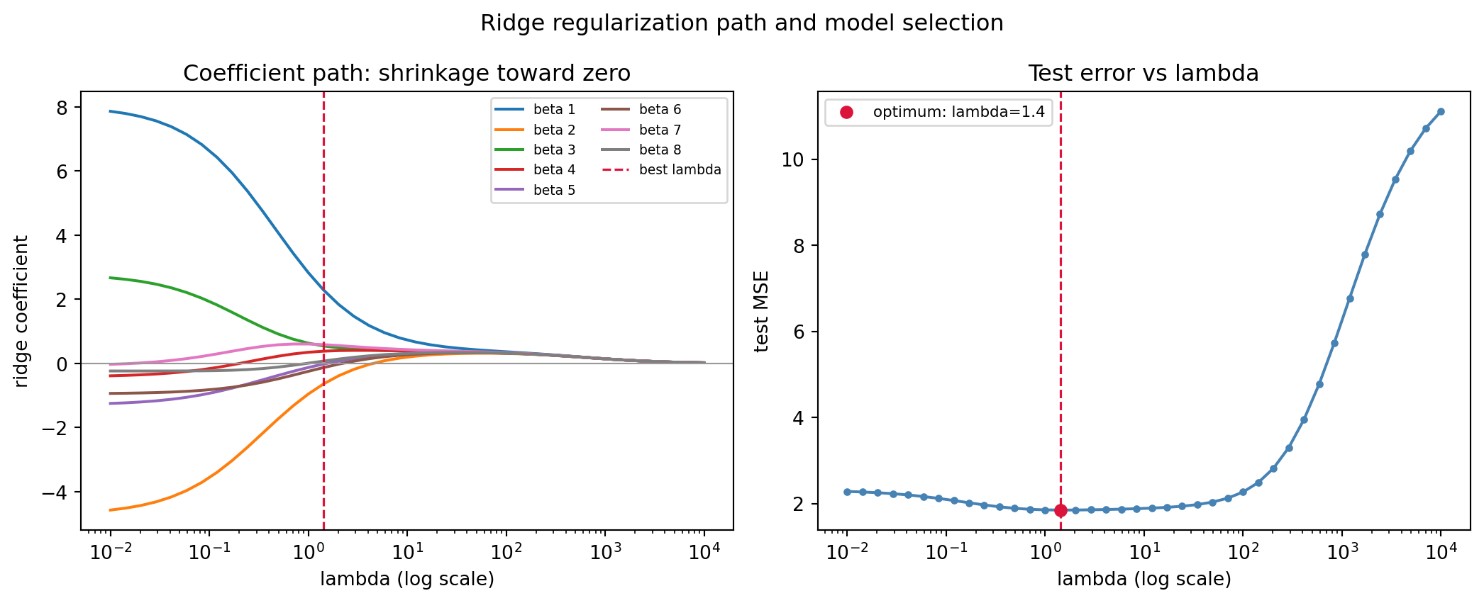
The following cell builds a synthetic regression with eight near collinear predictors, standardizes them, and sweeps \(\lambda\) across six orders of magnitude. It reports the OLS test error, the cross validation optimal \(\lambda\), the resulting effective degrees of freedom computed from the singular values, and the shrinkage in the coefficient norm. The seed is fixed so the output is reproducible.
Code
import numpy as npimport matplotlib.pyplot as pltfrom sklearn.linear_model import Ridgefrom sklearn.model_selection import train_test_splitrng = np.random.default_rng(0)# Synthetic problem with correlated predictors to stress OLSn, p =120, 8base = rng.standard_normal((n, 1))noise = rng.standard_normal((n, p))X =0.92* base +0.08* noise # columns share a common factor: near collinearX = (X - X.mean(0)) / X.std(0) # standardize each predictorbeta_true = np.array([3.0, -2.0, 0.0, 1.5, 0.0, 0.0, 2.0, -1.0])y = X @ beta_true +1.5* rng.standard_normal(n)y = y - y.mean()X_tr, X_te, y_tr, y_te = train_test_split(X, y, test_size=0.4, random_state=0)lambdas = np.logspace(-2, 4, 40)coefs, test_mse = [], []for lam in lambdas: m = Ridge(alpha=lam, fit_intercept=False).fit(X_tr, y_tr) coefs.append(m.coef_) test_mse.append(np.mean((y_te - m.predict(X_te)) **2))coefs = np.array(coefs)test_mse = np.array(test_mse)# Effective degrees of freedom via SVD of the training designd = np.linalg.svd(X_tr, compute_uv=False)def edf(lam):return np.sum(d**2/ (d**2+ lam))best =int(np.argmin(test_mse))print(f"OLS (lambda=0) test MSE: {test_mse[0]:.4f}")print(f"Best lambda: {lambdas[best]:.4g}")print(f"Best test MSE: {test_mse[best]:.4f}")print(f"Effective df at best lambda: {edf(lambdas[best]):.2f} (of p={p})")print(f"Coef L2 norm OLS vs best ridge: {np.linalg.norm(coefs[0]):.3f} -> {np.linalg.norm(coefs[best]):.3f}")# Visualize the ridge coefficient path and the test error curvefig, (ax_path, ax_err) = plt.subplots(1, 2, figsize=(11, 4.5))fig.suptitle("Ridge regularization path and model selection", fontsize=12)for j inrange(p): ax_path.plot(lambdas, coefs[:, j], label=f"beta {j+1}")ax_path.axhline(0.0, color="0.6", lw=0.8)ax_path.axvline(lambdas[best], color="crimson", ls="--", lw=1.2, label="best lambda")ax_path.set_xscale("log")ax_path.set_xlabel("lambda (log scale)")ax_path.set_ylabel("ridge coefficient")ax_path.set_title("Coefficient path: shrinkage toward zero")ax_path.legend(fontsize=7, ncol=2, loc="upper right")ax_err.plot(lambdas, test_mse, color="steelblue", marker="o", ms=3)ax_err.axvline(lambdas[best], color="crimson", ls="--", lw=1.2)ax_err.scatter([lambdas[best]], [test_mse[best]], color="crimson", zorder=5, label=f"optimum: lambda={lambdas[best]:.2g}")ax_err.set_xscale("log")ax_err.set_xlabel("lambda (log scale)")ax_err.set_ylabel("test MSE")ax_err.set_title("Test error vs lambda")ax_err.legend(fontsize=8, loc="upper left")fig.tight_layout()plt.show()
OLS (lambda=0) test MSE:        2.2798
Best lambda:                    1.425
Best test MSE:                  1.8474
Effective df at best lambda:    2.98  (of p=8)
Coef L2 norm OLS vs best ridge: 9.618 -> 2.545
Running this prints an OLS test MSE near \(2.28\) against a best ridge MSE near \(1.85\) at \(\lambda \approx 1.4\), where the effective degrees of freedom has collapsed from \(8\) to about \(3\) and the coefficient norm has shrunk from roughly \(9.6\) to \(2.5\). This is the bias variance tradeoff and the shrinkage view made concrete on one dataset.
89.6.2 6.2 The same computation in three languages
The closed form solve and the lambda sweep are short in any numerical language. The Python panel below is executable; the Julia and Rust panels are illustrative.
import numpy as npdef ridge_solve(X, y, lam): p = X.shape[1] A = X.T @ X + lam * np.eye(p) # positive definite b = X.T @ yreturn np.linalg.solve(A, b) # Cholesky-backed solve, never an explicit inversebeta_hat = ridge_solve(X_tr, y_tr, 1.0)print(np.round(beta_hat, 3))
usingLinearAlgebrafunctionridge_solve(X, y, lam) p =size(X, 2) A = X'* X + lam *I(p) # positive definite b = X'* yreturncholesky(Symmetric(A)) \ b # solve, no explicit inverseendbeta_hat =ridge_solve(X_tr, y_tr, 1.0)println(round.(beta_hat, digits =3))
// Illustrative: uses the `nalgebra` crateusenalgebra::{DMatrix, DVector};fn ridge_solve(x:&DMatrix<f64>, y:&DVector<f64>, lam:f64) -> DVector<f64>{let p = x.ncols();let a = x.transpose() * x + lam *DMatrix::identity(p, p);// positive definitelet b = x.transpose() * y; a.cholesky().expect("SPD").solve(&b) // solve, no explicit inverse}
89.7 7. Practical Guidance
Ridge is most valuable when predictors are correlated, when \(p\) is large relative to \(n\), or when the goal is stable prediction rather than interpretation of individual coefficients. Always center and scale the predictors first, and exclude the intercept from the penalty. Select \(\lambda\) by cross validation over a logarithmically spaced grid, since the useful range of \(\lambda\) spans many orders of magnitude. If sparsity or variable selection is the goal, the lasso or the elastic net is more appropriate, but for sheer predictive stability under collinearity ridge is often the better default, and the elastic net combines both penalties to capture grouped correlated predictors that ridge handles gracefully and the lasso does not. Modern libraries implement all of these efficiently, and the SVD of the design can be reused to evaluate the entire ridge path across \(\lambda\) values at almost no extra cost.
89.8 References
Hoerl, A. E., and Kennard, R. W. (1970). Ridge Regression: Biased Estimation for Nonorthogonal Problems. Technometrics, 12(1), 55 to 67. https://doi.org/10.1080/00401706.1970.10488634
Hoerl, A. E., and Kennard, R. W. (1970). Ridge Regression: Applications to Nonorthogonal Problems. Technometrics, 12(1), 69 to 82. https://doi.org/10.1080/00401706.1970.10488635
Golub, G. H., Heath, M., and Wahba, G. (1979). Generalized Cross Validation as a Method for Choosing a Good Ridge Parameter. Technometrics, 21(2), 215 to 223. https://doi.org/10.1080/00401706.1979.10489751
Zou, H., and Hastie, T. (2005). Regularization and Variable Selection via the Elastic Net. Journal of the Royal Statistical Society, Series B, 67(2), 301 to 320. https://doi.org/10.1111/j.1467-9868.2005.00503.x
Hastie, T., Tibshirani, R., and Friedman, J. (2009). The Elements of Statistical Learning, 2nd edition. Springer. https://doi.org/10.1007/978-0-387-84858-7
Pedregosa, F., et al. (2011). Scikit-learn: Machine Learning in Python. Journal of Machine Learning Research, 12, 2825 to 2830. https://jmlr.org/papers/v12/pedregosa11a.html
Murphy, K. P. (2022). Probabilistic Machine Learning: An Introduction. MIT Press. https://probml.github.io/pml-book/book1.html
Source Code
# Ridge Regression and L2 RegularizationOrdinary least squares is the workhorse of linear modeling, but it has a well known failure mode. When predictors are numerous, correlated, or nearly collinear, the least squares estimator becomes unstable: small perturbations in the data produce wildly different coefficient vectors, and predictions on new data degrade. Ridge regression, introduced by Hoerl and Kennard in 1970, addresses this by adding a quadratic penalty on the coefficient magnitudes. The result is a biased estimator that trades a small amount of bias for a large reduction in variance, and that remains well defined even when the design matrix is rank deficient. This chapter develops ridge regression from five complementary angles: the penalized objective, the closed form solution, the bias variance decomposition, the Bayesian interpretation as a Gaussian prior, and the shrinkage view through the singular value decomposition.## 1. The Penalized Objective### 1.1 Setup and notationLet $\mathbf{X} \in \mathbb{R}^{n \times p}$ denote the design matrix with $n$ observations and $p$ predictors, and let $\mathbf{y} \in \mathbb{R}^{n}$ denote the response vector. We seek a coefficient vector $\boldsymbol{\beta} \in \mathbb{R}^{p}$. Ordinary least squares (OLS) minimizes the residual sum of squares,$$\hat{\boldsymbol{\beta}}^{\text{OLS}} = \arg\min_{\boldsymbol{\beta}} \; \lVert \mathbf{y} - \mathbf{X}\boldsymbol{\beta} \rVert_2^2 .$$The OLS solution requires $\mathbf{X}^{\top}\mathbf{X}$ to be invertible. When $p > n$, or when columns of $\mathbf{X}$ are linearly dependent, this matrix is singular and the solution is not unique. Even when it is technically invertible, near collinearity makes $\mathbf{X}^{\top}\mathbf{X}$ ill conditioned, so the inverse amplifies noise.### 1.2 Adding the L2 penaltyRidge regression augments the objective with a penalty proportional to the squared Euclidean norm of the coefficients:$$\hat{\boldsymbol{\beta}}^{\text{ridge}}(\lambda) = \arg\min_{\boldsymbol{\beta}} \; \lVert \mathbf{y} - \mathbf{X}\boldsymbol{\beta} \rVert_2^2 + \lambda \lVert \boldsymbol{\beta} \rVert_2^2,$$where $\lambda \geq 0$ is the regularization strength. The term $\lambda \lVert \boldsymbol{\beta} \rVert_2^2 = \lambda \sum_{j=1}^{p} \beta_j^2$ discourages large coefficients. At $\lambda = 0$ we recover OLS. As $\lambda \to \infty$ the penalty dominates and every coefficient is driven toward zero.An equivalent formulation states ridge as a constrained problem,$$\hat{\boldsymbol{\beta}}^{\text{ridge}} = \arg\min_{\boldsymbol{\beta}} \; \lVert \mathbf{y} - \mathbf{X}\boldsymbol{\beta} \rVert_2^2 \quad \text{subject to} \quad \lVert \boldsymbol{\beta} \rVert_2^2 \leq t,$$with a one to one correspondence between $\lambda$ and the budget $t$. This geometric picture shows that ridge confines the solution to a Euclidean ball, and the smooth spherical boundary is why ridge shrinks coefficients continuously rather than setting them exactly to zero, in contrast to the L1 penalty of the lasso.### 1.3 The intercept and standardizationThe penalty should not apply to the intercept, since shrinking the intercept would make the fit depend on the arbitrary origin of the response. In practice we center $\mathbf{y}$ and each column of $\mathbf{X}$, fit a ridge model without an intercept on the centered data, and recover the intercept as $\hat{\beta}_0 = \bar{y}$ on the original scale. Furthermore, because the penalty $\sum_j \beta_j^2$ treats every coefficient equally, the solution is not invariant to the units of each predictor. A variable measured in millimeters receives a different penalty than the same variable in meters. The standard remedy is to standardize each predictor to unit variance before fitting, so that the penalty is applied on a common scale. These two preprocessing steps, centering and scaling, are essential for ridge to behave as intended.## 2. The Closed Form Solution### 2.1 Deriving the normal equationsThe ridge objective is a smooth convex quadratic in $\boldsymbol{\beta}$, so we find its minimizer by setting the gradient to zero. Write the objective as$$J(\boldsymbol{\beta}) = (\mathbf{y} - \mathbf{X}\boldsymbol{\beta})^{\top}(\mathbf{y} - \mathbf{X}\boldsymbol{\beta}) + \lambda \boldsymbol{\beta}^{\top}\boldsymbol{\beta} .$$Differentiating with respect to $\boldsymbol{\beta}$ gives$$\nabla_{\boldsymbol{\beta}} J = -2 \mathbf{X}^{\top}(\mathbf{y} - \mathbf{X}\boldsymbol{\beta}) + 2 \lambda \boldsymbol{\beta} .$$Setting this to zero yields the ridge normal equations,$$(\mathbf{X}^{\top}\mathbf{X} + \lambda \mathbf{I}_p)\,\boldsymbol{\beta} = \mathbf{X}^{\top}\mathbf{y},$$and therefore$$\hat{\boldsymbol{\beta}}^{\text{ridge}}(\lambda) = (\mathbf{X}^{\top}\mathbf{X} + \lambda \mathbf{I}_p)^{-1} \mathbf{X}^{\top}\mathbf{y} .$$### 2.2 Why the solution always existsThe matrix $\mathbf{X}^{\top}\mathbf{X}$ is symmetric positive semidefinite, so its eigenvalues are nonnegative. Adding $\lambda \mathbf{I}_p$ for any $\lambda > 0$ shifts every eigenvalue up by $\lambda$, making the eigenvalues strictly positive. The matrix $\mathbf{X}^{\top}\mathbf{X} + \lambda \mathbf{I}_p$ is therefore positive definite and invertible regardless of the rank of $\mathbf{X}$. This is the algebraic heart of ridge regularization. Even in the $p > n$ regime, where $\mathbf{X}^{\top}\mathbf{X}$ is singular, the ridge estimator is unique and stable. The penalty also improves the condition number: if $\mathbf{X}^{\top}\mathbf{X}$ has eigenvalues $d_j^2$, then the condition number drops from $d_{\max}^2 / d_{\min}^2$ to $(d_{\max}^2 + \lambda)/(d_{\min}^2 + \lambda)$, which is much closer to one when $\lambda$ is comparable to the smaller eigenvalues.### 2.3 Computational notesTwo practical formulations matter. When $p \leq n$, solving the $p \times p$ system above is efficient. When $p \gg n$, the Woodbury identity gives an equivalent expression that inverts an $n \times n$ matrix instead,$$\hat{\boldsymbol{\beta}}^{\text{ridge}} = \mathbf{X}^{\top}(\mathbf{X}\mathbf{X}^{\top} + \lambda \mathbf{I}_n)^{-1} \mathbf{y},$$which is cheaper in the high dimensional setting and exposes the kernel structure that underlies kernel ridge regression. In code, one should never form an explicit inverse; instead solve the linear system directly with a Cholesky factorization, since $\mathbf{X}^{\top}\mathbf{X} + \lambda \mathbf{I}$ is positive definite. Section 6 gives a runnable implementation.## 3. The Bias Variance Effect### 3.1 The decompositionFor a fixed test input $\mathbf{x}_0$, the expected squared prediction error decomposes into three parts: the irreducible noise variance, the squared bias of the estimator, and its variance. Ridge regression deliberately moves along this tradeoff. OLS is unbiased but can have enormous variance under collinearity. Ridge introduces bias by shrinking coefficients toward zero, but the variance reduction more than compensates over a useful range of $\lambda$, lowering the total expected error.### 3.2 Bias and variance of the ridge estimatorAssume the linear model $\mathbf{y} = \mathbf{X}\boldsymbol{\beta}^{\star} + \boldsymbol{\varepsilon}$ with $\mathbb{E}[\boldsymbol{\varepsilon}] = \mathbf{0}$ and $\operatorname{Cov}(\boldsymbol{\varepsilon}) = \sigma^2 \mathbf{I}$. Let $\mathbf{Z}_\lambda = (\mathbf{X}^{\top}\mathbf{X} + \lambda \mathbf{I})^{-1}\mathbf{X}^{\top}$, so that $\hat{\boldsymbol{\beta}}^{\text{ridge}} = \mathbf{Z}_\lambda \mathbf{y}$. Taking expectations,$$\mathbb{E}[\hat{\boldsymbol{\beta}}^{\text{ridge}}] = \mathbf{Z}_\lambda \mathbf{X}\boldsymbol{\beta}^{\star} = (\mathbf{X}^{\top}\mathbf{X} + \lambda \mathbf{I})^{-1}\mathbf{X}^{\top}\mathbf{X}\,\boldsymbol{\beta}^{\star} .$$The bias is$$\operatorname{Bias}(\hat{\boldsymbol{\beta}}^{\text{ridge}}) = -\lambda (\mathbf{X}^{\top}\mathbf{X} + \lambda \mathbf{I})^{-1}\boldsymbol{\beta}^{\star},$$which is zero only at $\lambda = 0$ and grows in magnitude with $\lambda$. The covariance is$$\operatorname{Cov}(\hat{\boldsymbol{\beta}}^{\text{ridge}}) = \sigma^2 \mathbf{Z}_\lambda \mathbf{Z}_\lambda^{\top} = \sigma^2 (\mathbf{X}^{\top}\mathbf{X} + \lambda \mathbf{I})^{-1}\mathbf{X}^{\top}\mathbf{X}(\mathbf{X}^{\top}\mathbf{X} + \lambda \mathbf{I})^{-1} .$$Each factor of $(\mathbf{X}^{\top}\mathbf{X} + \lambda \mathbf{I})^{-1}$ shrinks as $\lambda$ grows, so the variance decreases monotonically in $\lambda$. Bias increases while variance decreases, and the mean squared error is minimized at some intermediate $\lambda$.### 3.3 The existence theoremA central theoretical result, due to Hoerl and Kennard, is that there always exists a $\lambda > 0$ for which the ridge estimator has strictly smaller total mean squared error than OLS. In other words, OLS is never the optimal point on the bias variance curve. The catch is that the optimal $\lambda$ depends on the unknown true coefficients and noise level, so in practice it must be chosen from data, most commonly by $k$ fold cross validation or by generalized cross validation, which has an efficient leave one out form for ridge.## 4. The Bayesian Interpretation### 4.1 Gaussian likelihood and Gaussian priorRidge regression has a clean probabilistic reading as the maximum a posteriori (MAP) estimate under a Gaussian likelihood and a Gaussian prior on the coefficients. Suppose the data are generated as$$\mathbf{y} \mid \boldsymbol{\beta} \sim \mathcal{N}(\mathbf{X}\boldsymbol{\beta}, \, \sigma^2 \mathbf{I}_n),$$and place an independent zero mean Gaussian prior on each coefficient,$$\boldsymbol{\beta} \sim \mathcal{N}(\mathbf{0}, \, \tau^2 \mathbf{I}_p) .$$The prior encodes a belief that coefficients are small, with $\tau^2$ controlling how strongly we expect them to cluster around zero.### 4.2 The MAP estimate equals the ridge estimateBy Bayes' rule, the log posterior is the sum of the log likelihood and the log prior, up to a constant:$$\log p(\boldsymbol{\beta} \mid \mathbf{y}) = -\frac{1}{2\sigma^2}\lVert \mathbf{y} - \mathbf{X}\boldsymbol{\beta} \rVert_2^2 - \frac{1}{2\tau^2}\lVert \boldsymbol{\beta} \rVert_2^2 + \text{const} .$$Maximizing the posterior is equivalent to minimizing the negative log posterior. Multiplying by $2\sigma^2$ leaves the minimizer unchanged and yields exactly the ridge objective,$$\arg\max_{\boldsymbol{\beta}} \log p(\boldsymbol{\beta} \mid \mathbf{y}) = \arg\min_{\boldsymbol{\beta}} \; \lVert \mathbf{y} - \mathbf{X}\boldsymbol{\beta} \rVert_2^2 + \frac{\sigma^2}{\tau^2}\lVert \boldsymbol{\beta} \rVert_2^2 .$$The regularization parameter is therefore $\lambda = \sigma^2 / \tau^2$. A strong prior belief in small coefficients (small $\tau^2$) corresponds to large $\lambda$, while a diffuse prior (large $\tau^2$) corresponds to small $\lambda$, recovering OLS in the limit $\tau^2 \to \infty$.### 4.3 Beyond the point estimateBecause both the prior and the likelihood are Gaussian, the full posterior is itself Gaussian, with mean equal to the ridge estimate and covariance $(\sigma^{-2}\mathbf{X}^{\top}\mathbf{X} + \tau^{-2}\mathbf{I})^{-1}$. This is more than a curiosity. It means ridge is the posterior mean of a conjugate Bayesian linear model, so it delivers calibrated uncertainty intervals for free, and it connects directly to Gaussian process regression, where the same Gaussian prior is placed in a feature space. The Bayesian view also reframes the choice of $\lambda$ as a question of prior variance, which can be estimated by maximizing the marginal likelihood, an approach known as empirical Bayes or evidence maximization.## 5. The Shrinkage and SVD View### 5.1 Singular value decomposition of the designThe most illuminating analysis of ridge comes from the singular value decomposition (SVD) of the design matrix. Write$$\mathbf{X} = \mathbf{U}\mathbf{D}\mathbf{V}^{\top},$$where $\mathbf{U} \in \mathbb{R}^{n \times p}$ and $\mathbf{V} \in \mathbb{R}^{p \times p}$ have orthonormal columns and $\mathbf{D} = \operatorname{diag}(d_1, \ldots, d_p)$ holds the singular values $d_1 \geq d_2 \geq \cdots \geq d_p \geq 0$. The columns of $\mathbf{V}$ are the principal directions of the predictor space, and $d_j^2$ measures the variance of the data along direction $\mathbf{v}_j$.### 5.2 Ridge fitted values as filtered componentsTo derive the shrinkage form, substitute $\mathbf{X} = \mathbf{U}\mathbf{D}\mathbf{V}^{\top}$ into the closed form solution. Using the orthonormality $\mathbf{V}^{\top}\mathbf{V} = \mathbf{I}$, the penalized Gram matrix becomes$$\mathbf{X}^{\top}\mathbf{X} + \lambda \mathbf{I} = \mathbf{V}\mathbf{D}^2\mathbf{V}^{\top} + \lambda \mathbf{V}\mathbf{V}^{\top} = \mathbf{V}(\mathbf{D}^2 + \lambda \mathbf{I})\mathbf{V}^{\top},$$whose inverse is $\mathbf{V}(\mathbf{D}^2 + \lambda \mathbf{I})^{-1}\mathbf{V}^{\top}$ because $\mathbf{D}^2 + \lambda \mathbf{I}$ is diagonal. The coefficient vector is then$$\hat{\boldsymbol{\beta}}^{\text{ridge}} = \mathbf{V}(\mathbf{D}^2 + \lambda \mathbf{I})^{-1}\mathbf{V}^{\top}\mathbf{V}\mathbf{D}\mathbf{U}^{\top}\mathbf{y} = \mathbf{V}(\mathbf{D}^2 + \lambda \mathbf{I})^{-1}\mathbf{D}\,\mathbf{U}^{\top}\mathbf{y} = \sum_{j=1}^{p} \mathbf{v}_j \, \frac{d_j}{d_j^2 + \lambda}\, \mathbf{u}_j^{\top}\mathbf{y} .$$Left multiplying by $\mathbf{X} = \mathbf{U}\mathbf{D}\mathbf{V}^{\top}$ and again using $\mathbf{V}^{\top}\mathbf{V} = \mathbf{I}$, the diagonal term $d_j \cdot d_j/(d_j^2 + \lambda)$ collects into the shrinkage factor, so the ridge fitted values are$$\hat{\mathbf{y}}^{\text{ridge}} = \mathbf{X}\hat{\boldsymbol{\beta}}^{\text{ridge}} = \sum_{j=1}^{p} \mathbf{u}_j \, \frac{d_j^2}{d_j^2 + \lambda} \, \mathbf{u}_j^{\top}\mathbf{y} .$$Compare this with OLS, which uses the same expression but with every filter factor equal to one:$$\hat{\mathbf{y}}^{\text{OLS}} = \sum_{j=1}^{p} \mathbf{u}_j \, \mathbf{u}_j^{\top}\mathbf{y} .$$Ridge projects $\mathbf{y}$ onto each left singular vector $\mathbf{u}_j$ and then multiplies that component by the shrinkage factor$$f_j = \frac{d_j^2}{d_j^2 + \lambda} \in (0, 1) .$$### 5.3 Reading the shrinkage factorsThe factor $f_j$ reveals exactly how ridge acts. Directions with large singular values, where $d_j^2 \gg \lambda$, have $f_j \approx 1$ and are barely shrunk. Directions with small singular values, where $d_j^2 \ll \lambda$, have $f_j \approx d_j^2 / \lambda \approx 0$ and are shrunk heavily. Because $d_j^2$ is the variance of the data along $\mathbf{v}_j$, ridge preserves high variance directions and suppresses low variance directions. This is precisely where it helps: low variance directions are the ones along which collinearity makes the OLS coefficients explode, because dividing the projected response by a tiny $d_j$ amplifies noise. Ridge tempers that division by adding $\lambda$ to the denominator, so unstable directions are damped rather than amplified.### 5.4 Effective degrees of freedomThe shrinkage factors also give ridge a natural complexity measure. The hat matrix for ridge is $\mathbf{H}_\lambda = \mathbf{X}(\mathbf{X}^{\top}\mathbf{X} + \lambda \mathbf{I})^{-1}\mathbf{X}^{\top}$, and its trace is$$\operatorname{df}(\lambda) = \operatorname{tr}(\mathbf{H}_\lambda) = \sum_{j=1}^{p} \frac{d_j^2}{d_j^2 + \lambda} = \sum_{j=1}^{p} f_j .$$This effective degrees of freedom decreases smoothly from $p$ at $\lambda = 0$ toward zero as $\lambda \to \infty$, and it quantifies how many directions of the data the model is effectively using. It plays the role that the number of parameters plays in unregularized models, and it appears in model selection criteria and in the generalized cross validation score used to tune $\lambda$. The relationship to principal components analysis is direct: ridge is a soft version of principal components regression, which would set $f_j = 1$ for the top components and $f_j = 0$ for the rest, whereas ridge applies a smooth taper across all of them.## 6. Ridge in Code### 6.1 Coefficient path and test error (executable)The following cell builds a synthetic regression with eight near collinear predictors, standardizes them, and sweeps $\lambda$ across six orders of magnitude. It reports the OLS test error, the cross validation optimal $\lambda$, the resulting effective degrees of freedom computed from the singular values, and the shrinkage in the coefficient norm. The seed is fixed so the output is reproducible.```{python}import numpy as npimport matplotlib.pyplot as pltfrom sklearn.linear_model import Ridgefrom sklearn.model_selection import train_test_splitrng = np.random.default_rng(0)# Synthetic problem with correlated predictors to stress OLSn, p =120, 8base = rng.standard_normal((n, 1))noise = rng.standard_normal((n, p))X =0.92* base +0.08* noise # columns share a common factor: near collinearX = (X - X.mean(0)) / X.std(0) # standardize each predictorbeta_true = np.array([3.0, -2.0, 0.0, 1.5, 0.0, 0.0, 2.0, -1.0])y = X @ beta_true +1.5* rng.standard_normal(n)y = y - y.mean()X_tr, X_te, y_tr, y_te = train_test_split(X, y, test_size=0.4, random_state=0)lambdas = np.logspace(-2, 4, 40)coefs, test_mse = [], []for lam in lambdas: m = Ridge(alpha=lam, fit_intercept=False).fit(X_tr, y_tr) coefs.append(m.coef_) test_mse.append(np.mean((y_te - m.predict(X_te)) **2))coefs = np.array(coefs)test_mse = np.array(test_mse)# Effective degrees of freedom via SVD of the training designd = np.linalg.svd(X_tr, compute_uv=False)def edf(lam):return np.sum(d**2/ (d**2+ lam))best =int(np.argmin(test_mse))print(f"OLS (lambda=0) test MSE: {test_mse[0]:.4f}")print(f"Best lambda: {lambdas[best]:.4g}")print(f"Best test MSE: {test_mse[best]:.4f}")print(f"Effective df at best lambda: {edf(lambdas[best]):.2f} (of p={p})")print(f"Coef L2 norm OLS vs best ridge: {np.linalg.norm(coefs[0]):.3f} -> {np.linalg.norm(coefs[best]):.3f}")# Visualize the ridge coefficient path and the test error curvefig, (ax_path, ax_err) = plt.subplots(1, 2, figsize=(11, 4.5))fig.suptitle("Ridge regularization path and model selection", fontsize=12)for j inrange(p): ax_path.plot(lambdas, coefs[:, j], label=f"beta {j+1}")ax_path.axhline(0.0, color="0.6", lw=0.8)ax_path.axvline(lambdas[best], color="crimson", ls="--", lw=1.2, label="best lambda")ax_path.set_xscale("log")ax_path.set_xlabel("lambda (log scale)")ax_path.set_ylabel("ridge coefficient")ax_path.set_title("Coefficient path: shrinkage toward zero")ax_path.legend(fontsize=7, ncol=2, loc="upper right")ax_err.plot(lambdas, test_mse, color="steelblue", marker="o", ms=3)ax_err.axvline(lambdas[best], color="crimson", ls="--", lw=1.2)ax_err.scatter([lambdas[best]], [test_mse[best]], color="crimson", zorder=5, label=f"optimum: lambda={lambdas[best]:.2g}")ax_err.set_xscale("log")ax_err.set_xlabel("lambda (log scale)")ax_err.set_ylabel("test MSE")ax_err.set_title("Test error vs lambda")ax_err.legend(fontsize=8, loc="upper left")fig.tight_layout()plt.show()```Running this prints an OLS test MSE near $2.28$ against a best ridge MSE near $1.85$ at $\lambda \approx 1.4$, where the effective degrees of freedom has collapsed from $8$ to about $3$ and the coefficient norm has shrunk from roughly $9.6$ to $2.5$. This is the bias variance tradeoff and the shrinkage view made concrete on one dataset.### 6.2 The same computation in three languagesThe closed form solve and the lambda sweep are short in any numerical language. The Python panel below is executable; the Julia and Rust panels are illustrative.::: {.panel-tabset}## Python```{python}import numpy as npdef ridge_solve(X, y, lam): p = X.shape[1] A = X.T @ X + lam * np.eye(p) # positive definite b = X.T @ yreturn np.linalg.solve(A, b) # Cholesky-backed solve, never an explicit inversebeta_hat = ridge_solve(X_tr, y_tr, 1.0)print(np.round(beta_hat, 3))```## Julia```juliausingLinearAlgebrafunctionridge_solve(X, y, lam) p =size(X, 2) A = X'* X + lam *I(p) # positive definite b = X'* yreturncholesky(Symmetric(A)) \ b # solve, no explicit inverseendbeta_hat =ridge_solve(X_tr, y_tr, 1.0)println(round.(beta_hat, digits =3))```## Rust```rust// Illustrative: uses the `nalgebra` crateuse nalgebra::{DMatrix, DVector};fn ridge_solve(x:&DMatrix<f64>, y:&DVector<f64>, lam: f64) -> DVector<f64> { let p =x.ncols(); let a =x.transpose() * x + lam * DMatrix::identity(p, p); // positive definite let b =x.transpose() * y;a.cholesky().expect("SPD").solve(&b) // solve, no explicit inverse}```:::## 7. Practical GuidanceRidge is most valuable when predictors are correlated, when $p$ is large relative to $n$, or when the goal is stable prediction rather than interpretation of individual coefficients. Always center and scale the predictors first, and exclude the intercept from the penalty. Select $\lambda$ by cross validation over a logarithmically spaced grid, since the useful range of $\lambda$ spans many orders of magnitude. If sparsity or variable selection is the goal, the lasso or the elastic net is more appropriate, but for sheer predictive stability under collinearity ridge is often the better default, and the elastic net combines both penalties to capture grouped correlated predictors that ridge handles gracefully and the lasso does not. Modern libraries implement all of these efficiently, and the SVD of the design can be reused to evaluate the entire ridge path across $\lambda$ values at almost no extra cost.## References1. Hoerl, A. E., and Kennard, R. W. (1970). Ridge Regression: Biased Estimation for Nonorthogonal Problems. Technometrics, 12(1), 55 to 67. https://doi.org/10.1080/00401706.1970.104886342. Hoerl, A. E., and Kennard, R. W. (1970). Ridge Regression: Applications to Nonorthogonal Problems. Technometrics, 12(1), 69 to 82. https://doi.org/10.1080/00401706.1970.104886353. Golub, G. H., Heath, M., and Wahba, G. (1979). Generalized Cross Validation as a Method for Choosing a Good Ridge Parameter. Technometrics, 21(2), 215 to 223. https://doi.org/10.1080/00401706.1979.104897514. Zou, H., and Hastie, T. (2005). Regularization and Variable Selection via the Elastic Net. Journal of the Royal Statistical Society, Series B, 67(2), 301 to 320. https://doi.org/10.1111/j.1467-9868.2005.00503.x5. Hastie, T., Tibshirani, R., and Friedman, J. (2009). The Elements of Statistical Learning, 2nd edition. Springer. https://doi.org/10.1007/978-0-387-84858-76. Pedregosa, F., et al. (2011). Scikit-learn: Machine Learning in Python. Journal of Machine Learning Research, 12, 2825 to 2830. https://jmlr.org/papers/v12/pedregosa11a.html7. Murphy, K. P. (2022). Probabilistic Machine Learning: An Introduction. MIT Press. https://probml.github.io/pml-book/book1.html