For decades, statistical learning theory was governed by a single, intuitive rule: the Bias-Variance Trade-off. This rule suggested that as you increase a model’s complexity (e.g., adding more parameters or layers), the model eventually begins to “overfit.” It memorizes the noise in the training data rather than the signal. Consequently, while training error goes to zero, the test error (performance on new data) begins to explode.
This created a “U-shaped” curve for test error. The goal of a data scientist was to find the “sweet spot” at the bottom of the U, balancing underfitting (high bias) and overfitting (high variance).
However, modern deep learning broke this rule. Neural networks with millions (or billions) of parameters (i.e., far more than the number of training data points) often achieve state-of-the-art performance without overfitting in the traditional sense. They achieve zero training error yet still generalize remarkably well.
Double Descent is the phenomenon that reconciles these two worlds. As described by Belkin et al. (2019), if we continue to increase model complexity far beyond the point of overfitting, the test error drops a second time.
This chapter explores why this happens, the role of the “interpolation threshold,” and the mathematical mechanics of the minimum-norm solution.
44.2 The Phenomenon: Three Regimes
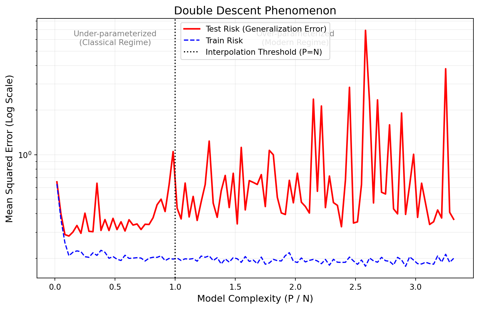
The Double Descent curve describes test error as a function of model complexity (specifically, the ratio of parameters \(P\) to samples \(N\)). It consists of two valleys separated by a peak.
44.2.1 The Classical Regime (\(P < N\))
This is the “under-parameterized” zone. We have fewer parameters than data points. * Behavior: As complexity increases, the model fits the data better. Bias decreases, and variance increases slightly. Test error drops. * Math: The system is over-determined. We solve it using standard Least Squares: \(\hat{\beta} = (X^T X)^{-1} X^T y\).
44.2.2 The Critical Regime (\(P \approx N\))
This is the “interpolation threshold.” The number of parameters roughly equals the number of data points. * Behavior: The model has just enough freedom to fit every single data point perfectly, including the noise. * The Peak: To hit every noisy data point exactly, the model must contort itself wildly. The weights (\(\beta\)) usually explode in magnitude. This leads to massive variance and a spike in test error. * Condition Number: As noted in related literature (Loog et al. 2020), this peak often correlates with the singularity of the data matrix. The matrix \(X^T X\) becomes nearly non-invertible, causing numerical instability and noise amplification.
44.2.3 The Modern Regime (\(P > N\))
This is the “over-parameterized” zone. We have far more parameters than data points.
Behavior: The model can still fit the training data perfectly (zero training error). However, because there are infinite solutions that fit the data, the solver (like SGD) implicitly chooses the “simplest” one, typically the one with the smallest Euclidean norm (smallest weights).
The Second Descent: As \(P\) increases further to infinity, the “space” of solutions grows. By distributing the “energy” of the solution across many dimensions, the model becomes smoother and more robust to noise. The test error drops again, often lower than the classical minimum.
44.3 Mathematical Intuition: The Minimum Norm Solution
Why does adding more parameters help reduce overfitting?
In the over-parameterized regime (\(P > N\)), the system \(X\beta = y\) has infinite solutions. Standard Gradient Descent initializes at zero and moves toward the solution. This trajectory converges specifically to the minimum\(\ell_2\)-norm solution:
\[
\hat{\beta}_{min-norm} = \text{argmin}_{\beta} \|\beta\|_2 \quad \text{subject to } X\beta = y
\]
Mathematically, this solution is given by the Moore-Penrose pseudo-inverse:
\[
\hat{\beta} = X^T (XX^T)^{-1} y
\]
44.3.1 The Intuition of “Jamming”
Imagine trying to fit a curve through 10 noisy data points.
Classical (\(P=3\)): A quadratic curve. It ignores noise but might miss the trend.
Critical (\(P=10\)): A 9th-degree polynomial. It must pass through every point. To do so, it oscillates violently between points. This is the peak of the Double Descent.
Modern (\(P=1000\)): We have 1000 parameters. We still hit the 10 points. But among the infinite curves that hit those points, we choose the “flattest” or “smoothest” one (minimum norm). As \(P \to \infty\), this solution actually converges back to a stable, well-behaved function that generalizes well. The “extra” dimensions act as a buffer that absorbs the noise without distorting the global shape.
44.4 Simulation in Python
We will simulate this phenomenon using a “Random Fourier Features” model, which is a standard proxy for neural networks in theoretical analysis. We will regress a simple sine wave with added noise.
44.4.1 Setup
Target Function:\(y = \sin(x) + \epsilon\)
Model: Linear regression on \(P\) random Fourier features.
Varying: We will vary \(P\) (number of features) from 1 to 200, while keeping \(N\) (samples) fixed at 60.
Code
import numpy as npimport matplotlib.pyplot as pltfrom sklearn.linear_model import Ridgefrom sklearn.metrics import mean_squared_errorfrom sklearn.model_selection import train_test_split# Set random seed for reproducibilitynp.random.seed(42)def generate_data(n_samples, noise_level=0.5):"""Generates synthetic data y = sin(x) + noise.""" X = np.random.uniform(-np.pi, np.pi, (n_samples, 1)) y = np.sin(X).ravel() + np.random.normal(0, noise_level, n_samples)return X, yclass RandomFourierFeatures:""" A simple model that projects input X into a high-dimensional feature space using random weights, then performs linear regression. This mimics a 1-hidden-layer neural network with fixed first layer. """def__init__(self, n_features, ridge_alpha=1e-8):self.n_features = n_featuresself.alpha = ridge_alphaself.W =Noneself.b =Noneself.coef_ =Nonedef fit(self, X, y): n_samples, n_input = X.shape# 1. Random projection (fixed, not learned)# We sample weights from a normal distributionself.W = np.random.normal(0, 1, (n_input, self.n_features))self.b = np.random.uniform(0, 2*np.pi, self.n_features)# 2. Transform input to feature space: Z = cos(XW + b) Z = np.cos(X @self.W +self.b)# 3. Solve Linear Regression (Ridge with tiny alpha for numerical stability)# In the interpolation regime, this approximates the min-norm solution. ridge = Ridge(alpha=self.alpha, fit_intercept=False) ridge.fit(Z, y)self.coef_ = ridge.coef_def predict(self, X): Z = np.cos(X @self.W +self.b)return Z @self.coef_# --- Experiment Parameters ---N_TRAIN =60N_TEST =1000feature_counts = np.arange(1, 200, 2) # Testing complexities from P=1 to P=200trials =20# Average over multiple trials to smooth the curve# Storage for resultstrain_risks = []test_risks = []param_ratios = []X_test, y_test = generate_data(N_TEST, noise_level=0.5)print(f"Running simulation with N={N_TRAIN} samples...")for P in feature_counts: trial_train_err = [] trial_test_err = []for _ inrange(trials): X_train, y_train = generate_data(N_TRAIN, noise_level=0.5) model = RandomFourierFeatures(n_features=P) model.fit(X_train, y_train)# Calculate MSE y_pred_train = model.predict(X_train) y_pred_test = model.predict(X_test) trial_train_err.append(mean_squared_error(y_train, y_pred_train)) trial_test_err.append(mean_squared_error(y_test, y_pred_test))# Average over trials train_risks.append(np.mean(trial_train_err)) test_risks.append(np.mean(trial_test_err)) param_ratios.append(P / N_TRAIN)# --- Visualization ---plt.figure(figsize=(10, 6))# Plot Test Riskplt.plot(param_ratios, test_risks, label='Test Risk (Generalization Error)', color='red', linewidth=2)# Plot Train Riskplt.plot(param_ratios, train_risks, label='Train Risk', color='blue', linestyle='--', linewidth=1.5)# Add Interpolation Threshold lineplt.axvline(x=1.0, color='black', linestyle=':', label='Interpolation Threshold (P=N)')# Annotations for the regimesplt.text(0.5, max(test_risks)*0.8, 'Under-parameterized\n(Classical Regime)', ha='center', fontsize=10, color='gray')plt.text(2.0, max(test_risks)*0.8, 'Over-parameterized\n(Modern Regime)', ha='center', fontsize=10, color='gray')plt.xlabel('Model Complexity (P / N)', fontsize=12)plt.ylabel('Mean Squared Error (Log Scale)', fontsize=12)plt.title('Double Descent Phenomenon', fontsize=14)plt.yscale('log') # Log scale is crucial to see the descent clearlyplt.legend()plt.grid(True, which="both", ls="-", alpha=0.2)plt.show()
Running simulation with N=60 samples...
44.5 Analysis of the Results
The plot generated above should clearly display the three key phases:
The First Descent: As goes from 0 to 1, the training error drops, and test error drops initially. This is the classical bias reduction.
The Peak: At, the training error hits zero (or near zero), but the test error spikes dramatically. This is where the model is “jammed.” It is forced to fit the noise with a unique but unstable solution.
The Second Descent: As, the training error stays at zero. Remarkably, the test error begins to decrease again. The implicit regularization of the high-dimensional space smooths out the function.
44.5.1 Connection to Random Matrix Theory
Poggio, Kur, and Banburski (2019) highlight that the spike in error at is driven by the smallest singular value of the data matrix approaching zero.
When, the random feature matrix is square. Random square matrices are known to have a non-trivial probability of having very small eigenvalues. Since the least-squares solution involves inverting these eigenvalues (), a small eigenvalue results in a massive amplification of the label noise ().
When, the matrix becomes a “wide” rectangular matrix. Random Matrix Theory (specifically the Marchenko-Pastur law) tells us that the singular values of wide random matrices are well-bounded away from zero. This means the pseudo-inverse is stable, the noise is not amplified, and the model generalizes well.
44.6 Conclusion
Double Descent challenges the classical dogma that “smaller models are better.” It suggests that there are two ways to achieve low error:
Classical: Keep the model small () to control variance.
Modern: Make the model huge () and rely on the implicit regularization of the optimization algorithm (minimum norm solution).
This insight explains why massive Deep Learning models (like Transformers or ResNets) work so well despite having far more parameters than training samples. They operate comfortably on the right side of the Double Descent curve.
Belkin, Mikhail, Daniel Hsu, Siyuan Ma, and Soumik Mandal. 2019. “Reconciling Modern Machine-Learning Practice and the Classical Bias–Variance Trade-Off.”Proceedings of the National Academy of Sciences 116 (32): 15849–54.
Loog, Marco, Tom Viering, Alexander Mey, Jesse H Krijthe, and David MJ Tax. 2020. “A Brief Prehistory of Double Descent.”Proceedings of the National Academy of Sciences 117 (20): 10625–26.
Poggio, Tomaso, Gil Kur, and Andrzej Banburski. 2019. “Double Descent in the Condition Number.”arXiv Preprint arXiv:1912.06190.
Source Code
# Double Descent## Introduction: The ConflictFor decades, statistical learning theory was governed by a single, intuitive rule: the **Bias-Variance Trade-off**. This rule suggested that as you increase a model's complexity (e.g., adding more parameters or layers), the model eventually begins to "overfit." It memorizes the noise in the training data rather than the signal. Consequently, while training error goes to zero, the test error (performance on new data) begins to explode.This created a "U-shaped" curve for test error. The goal of a data scientist was to find the "sweet spot" at the bottom of the U, balancing underfitting (high bias) and overfitting (high variance).However, modern deep learning broke this rule. Neural networks with millions (or billions) of parameters (i.e., far more than the number of training data points) often achieve state-of-the-art performance without overfitting in the traditional sense. They achieve zero training error yet still generalize remarkably well.**Double Descent** is the phenomenon that reconciles these two worlds. As described by @belkin2019reconciling, if we continue to increase model complexity far beyond the point of overfitting, the test error drops a *second* time.This chapter explores why this happens, the role of the "interpolation threshold," and the mathematical mechanics of the minimum-norm solution.## The Phenomenon: Three RegimesThe Double Descent curve describes test error as a function of model complexity (specifically, the ratio of parameters $P$ to samples $N$). It consists of two valleys separated by a peak.### The Classical Regime **(**$P < N$**)**This is the "under-parameterized" zone. We have fewer parameters than data points. \* **Behavior:** As complexity increases, the model fits the data better. Bias decreases, and variance increases slightly. Test error drops. \* **Math:** The system is over-determined. We solve it using standard Least Squares: $\hat{\beta} = (X^T X)^{-1} X^T y$.### The Critical Regime ($P \approx N$)This is the "interpolation threshold." The number of parameters roughly equals the number of data points. \* **Behavior:** The model has just enough freedom to fit every single data point perfectly, including the noise. \* **The Peak:** To hit every noisy data point exactly, the model must contort itself wildly. The weights ($\beta$) usually explode in magnitude. This leads to massive variance and a spike in test error. \* **Condition Number:** As noted in related literature [@loog2020brief], this peak often correlates with the singularity of the data matrix. The matrix $X^T X$ becomes nearly non-invertible, causing numerical instability and noise amplification.### The Modern Regime ($P > N$)This is the "over-parameterized" zone. We have far more parameters than data points.- **Behavior:** The model can still fit the training data perfectly (zero training error). However, because there are infinite solutions that fit the data, the solver (like SGD) implicitly chooses the "simplest" one, typically the one with the smallest Euclidean norm (smallest weights).- **The Second Descent:** As $P$ increases further to infinity, the "space" of solutions grows. By distributing the "energy" of the solution across many dimensions, the model becomes smoother and more robust to noise. The test error drops again, often lower than the classical minimum.## Mathematical Intuition: The Minimum Norm SolutionWhy does adding *more* parameters help reduce overfitting?In the over-parameterized regime ($P > N$), the system $X\beta = y$ has infinite solutions. Standard Gradient Descent initializes at zero and moves toward the solution. This trajectory converges specifically to the **minimum** $\ell_2$-norm solution:$$\hat{\beta}_{min-norm} = \text{argmin}_{\beta} \|\beta\|_2 \quad \text{subject to } X\beta = y$$Mathematically, this solution is given by the Moore-Penrose pseudo-inverse:$$\hat{\beta} = X^T (XX^T)^{-1} y$$### The Intuition of "Jamming"Imagine trying to fit a curve through 10 noisy data points.1. **Classical** ($P=3$): A quadratic curve. It ignores noise but might miss the trend.2. **Critical** ($P=10$): A 9th-degree polynomial. It *must* pass through every point. To do so, it oscillates violently between points. This is the peak of the Double Descent.3. **Modern** ($P=1000$): We have 1000 parameters. We still hit the 10 points. But among the infinite curves that hit those points, we choose the "flattest" or "smoothest" one (minimum norm). As $P \to \infty$, this solution actually converges back to a stable, well-behaved function that generalizes well. The "extra" dimensions act as a buffer that absorbs the noise without distorting the global shape.## Simulation in PythonWe will simulate this phenomenon using a "Random Fourier Features" model, which is a standard proxy for neural networks in theoretical analysis. We will regress a simple sine wave with added noise.### Setup- **Target Function:** $y = \sin(x) + \epsilon$- **Model:** Linear regression on $P$ random Fourier features.- **Varying:** We will vary $P$ (number of features) from 1 to 200, while keeping $N$ (samples) fixed at 60.```{python}import numpy as npimport matplotlib.pyplot as pltfrom sklearn.linear_model import Ridgefrom sklearn.metrics import mean_squared_errorfrom sklearn.model_selection import train_test_split# Set random seed for reproducibilitynp.random.seed(42)def generate_data(n_samples, noise_level=0.5):"""Generates synthetic data y = sin(x) + noise.""" X = np.random.uniform(-np.pi, np.pi, (n_samples, 1)) y = np.sin(X).ravel() + np.random.normal(0, noise_level, n_samples)return X, yclass RandomFourierFeatures:""" A simple model that projects input X into a high-dimensional feature space using random weights, then performs linear regression. This mimics a 1-hidden-layer neural network with fixed first layer. """def__init__(self, n_features, ridge_alpha=1e-8):self.n_features = n_featuresself.alpha = ridge_alphaself.W =Noneself.b =Noneself.coef_ =Nonedef fit(self, X, y): n_samples, n_input = X.shape# 1. Random projection (fixed, not learned)# We sample weights from a normal distributionself.W = np.random.normal(0, 1, (n_input, self.n_features))self.b = np.random.uniform(0, 2*np.pi, self.n_features)# 2. Transform input to feature space: Z = cos(XW + b) Z = np.cos(X @self.W +self.b)# 3. Solve Linear Regression (Ridge with tiny alpha for numerical stability)# In the interpolation regime, this approximates the min-norm solution. ridge = Ridge(alpha=self.alpha, fit_intercept=False) ridge.fit(Z, y)self.coef_ = ridge.coef_def predict(self, X): Z = np.cos(X @self.W +self.b)return Z @self.coef_# --- Experiment Parameters ---N_TRAIN =60N_TEST =1000feature_counts = np.arange(1, 200, 2) # Testing complexities from P=1 to P=200trials =20# Average over multiple trials to smooth the curve# Storage for resultstrain_risks = []test_risks = []param_ratios = []X_test, y_test = generate_data(N_TEST, noise_level=0.5)print(f"Running simulation with N={N_TRAIN} samples...")for P in feature_counts: trial_train_err = [] trial_test_err = []for _ inrange(trials): X_train, y_train = generate_data(N_TRAIN, noise_level=0.5) model = RandomFourierFeatures(n_features=P) model.fit(X_train, y_train)# Calculate MSE y_pred_train = model.predict(X_train) y_pred_test = model.predict(X_test) trial_train_err.append(mean_squared_error(y_train, y_pred_train)) trial_test_err.append(mean_squared_error(y_test, y_pred_test))# Average over trials train_risks.append(np.mean(trial_train_err)) test_risks.append(np.mean(trial_test_err)) param_ratios.append(P / N_TRAIN)# --- Visualization ---plt.figure(figsize=(10, 6))# Plot Test Riskplt.plot(param_ratios, test_risks, label='Test Risk (Generalization Error)', color='red', linewidth=2)# Plot Train Riskplt.plot(param_ratios, train_risks, label='Train Risk', color='blue', linestyle='--', linewidth=1.5)# Add Interpolation Threshold lineplt.axvline(x=1.0, color='black', linestyle=':', label='Interpolation Threshold (P=N)')# Annotations for the regimesplt.text(0.5, max(test_risks)*0.8, 'Under-parameterized\n(Classical Regime)', ha='center', fontsize=10, color='gray')plt.text(2.0, max(test_risks)*0.8, 'Over-parameterized\n(Modern Regime)', ha='center', fontsize=10, color='gray')plt.xlabel('Model Complexity (P / N)', fontsize=12)plt.ylabel('Mean Squared Error (Log Scale)', fontsize=12)plt.title('Double Descent Phenomenon', fontsize=14)plt.yscale('log') # Log scale is crucial to see the descent clearlyplt.legend()plt.grid(True, which="both", ls="-", alpha=0.2)plt.show()```## Analysis of the ResultsThe plot generated above should clearly display the three key phases:1. **The First Descent:** As goes from 0 to 1, the training error drops, and test error drops initially. This is the classical bias reduction.2. **The Peak:** At, the training error hits zero (or near zero), but the test error spikes dramatically. This is where the model is "jammed." It is forced to fit the noise with a unique but unstable solution.3. **The Second Descent:** As, the training error stays at zero. Remarkably, the test error begins to decrease again. The implicit regularization of the high-dimensional space smooths out the function.### Connection to Random Matrix Theory@poggio2019double highlight that the spike in error at is driven by the smallest singular value of the data matrix approaching zero.When, the random feature matrix is square. Random square matrices are known to have a non-trivial probability of having very small eigenvalues. Since the least-squares solution involves inverting these eigenvalues (), a small eigenvalue results in a massive amplification of the label noise ().When, the matrix becomes a "wide" rectangular matrix. Random Matrix Theory (specifically the Marchenko-Pastur law) tells us that the singular values of wide random matrices are well-bounded away from zero. This means the pseudo-inverse is stable, the noise is not amplified, and the model generalizes well.## ConclusionDouble Descent challenges the classical dogma that "smaller models are better." It suggests that there are two ways to achieve low error:1. **Classical:** Keep the model small () to control variance.2. **Modern:** Make the model huge () and rely on the implicit regularization of the optimization algorithm (minimum norm solution).This insight explains why massive Deep Learning models (like Transformers or ResNets) work so well despite having far more parameters than training samples. They operate comfortably on the right side of the Double Descent curve.