Hypothesis testing is the formal machinery that statistics offers for deciding whether a pattern in data reflects a real effect or could plausibly be the product of chance alone. For practitioners of machine learning, this machinery is both indispensable and dangerous. It is indispensable because almost every claim we make about a model, that one architecture beats another, that a feature improves accuracy, that a deployment shift is real and not noise, is at bottom a statistical claim. It is dangerous because the formalism is widely misunderstood, and the misunderstandings are precisely the ones that lead to overconfident, irreproducible conclusions. This chapter develops the logic of hypothesis testing carefully, defines its core quantities, catalogs the most common tests, and then turns to how the framework is applied and abused when we compare machine learning models.
38.1 1. The Logic of Null and Alternative Hypotheses
38.1.1 1.1 The two hypotheses
A hypothesis test begins by partitioning the possible states of the world into two complementary claims. The null hypothesis, written \(H_0\), is a specific statement that there is no effect, no difference, or no relationship. The alternative hypothesis, written \(H_1\) or \(H_a\), is the claim we entertain if the null is found implausible. The asymmetry between them is deliberate and important. The null is the default, the position of skepticism that we hold until the data force us to abandon it. The test is constructed so that we either reject \(H_0\) in favor of \(H_1\), or fail to reject \(H_0\). We never accept \(H_0\) as proven true.
Concretely, suppose we measure the difference in mean accuracy between two classifiers across a set of test instances. A natural null is that the true mean difference is zero,
\[H_0: \mu_A - \mu_B = 0,\]
against the two-sided alternative
\[H_1: \mu_A - \mu_B \neq 0.\]
If we had a directional prior belief, for instance that model \(A\) can only help, we might instead use the one-sided alternative \(H_1: \mu_A - \mu_B > 0\). The choice of one-sided versus two-sided must be made before seeing the data, because switching after the fact silently doubles the effective error rate.
38.1.2 1.2 Why we reason from the null
The reason we frame everything around a null of no effect is that the null is usually a sharp, fully specified hypothesis. Under \(H_0\) we can often compute, exactly or approximately, the distribution of any statistic we choose to measure. The alternative, by contrast, is typically composite: it covers a whole range of possible effect sizes, and we cannot compute a single sampling distribution for it without committing to one specific value. Hypothesis testing therefore proceeds by assuming the null is true, asking how surprising the observed data would be under that assumption, and rejecting the null only when the data are surprising enough.
38.1.3 1.3 The Neyman-Pearson framework
Two distinct philosophies underlie modern testing, and conflating them is the root of much confusion. Fisher treated the p-value as a continuous measure of evidence against the null, to be weighed by judgment. Neyman and Pearson recast testing as a decision procedure with controlled long-run error rates [1]. In their formulation we fix in advance a significance level \(\alpha\), partition the sample space into a rejection region \(R\) and its complement, and adopt the rule: reject \(H_0\) if and only if the data fall in \(R\). The region is chosen so that the false positive rate is controlled,
\[P(\text{data} \in R \mid H_0) \leq \alpha,\]
and, subject to that constraint, the power \(P(\text{data} \in R \mid H_1)\) is made as large as possible.
The cornerstone result is the Neyman-Pearson lemma. For testing a simple null \(H_0: \theta = \theta_0\) against a simple alternative \(H_1: \theta = \theta_1\), the most powerful test of level \(\alpha\) rejects when the likelihood ratio exceeds a threshold,
with \(k\) chosen so that \(P(\Lambda \geq k \mid H_0) = \alpha\). No other test with the same Type I error rate achieves higher power. This lemma is why so many standard tests, the \(z\)-test and \(t\)-test among them, take the form of comparing a statistic against a critical threshold: they are likelihood-ratio tests in disguise, and their rejection regions are optimal. The practical reading is that a test is a fixed rule chosen before the data arrive, and its quality is judged by two numbers, its size \(\alpha\) and its power, not by the particular p-value it happens to return on one dataset.
38.2 2. Test Statistics and Their Sampling Distributions
38.2.1 2.1 From data to a single number
A test statistic is a function of the data that summarizes the evidence relevant to the hypotheses into a single number, and whose distribution under \(H_0\) is known. The art of designing a test lies in choosing a statistic that is sensitive to the alternative, large when \(H_1\) holds, yet has a tractable distribution when \(H_0\) holds.
The canonical example is the one-sample \(t\) statistic. Given \(n\) observations \(x_1, \dots, x_n\) with sample mean \(\bar{x}\) and sample standard deviation \(s\), and a null value \(\mu_0\), we form
\[t = \frac{\bar{x} - \mu_0}{s / \sqrt{n}}.\]
The numerator measures how far the observed mean sits from the null value, and the denominator, the standard error of the mean, rescales that distance into units of sampling variability. If the null holds and the data are approximately normal, this statistic follows a Student \(t\) distribution with \(n - 1\) degrees of freedom.
38.2.2 2.2 The sampling distribution
The key conceptual object is the sampling distribution: the distribution of the test statistic across hypothetical repetitions of the experiment, assuming \(H_0\) is true. We almost never observe this distribution directly. Instead we derive it from theory, as with the \(t\) and chi-squared families, or we approximate it through resampling methods such as the permutation test and the bootstrap. Once we know the sampling distribution, the observed value of the statistic can be placed on it, and we can ask how far into the tail it falls.
The simplest null distribution to reason about is that of the \(z\)-statistic. Suppose we observe \(n\) independent draws from a population with unknown mean \(\mu\) but known standard deviation \(\sigma\), and we test \(H_0: \mu = \mu_0\). The standardized statistic
\[Z = \frac{\bar{X} - \mu_0}{\sigma / \sqrt{n}}\]
has, under \(H_0\), exactly the standard normal distribution \(Z \sim \mathcal{N}(0, 1)\), because \(\bar{X} \sim \mathcal{N}(\mu_0, \sigma^2/n)\) and subtracting the mean and dividing by the standard deviation of a normal random variable produces a standard normal. When \(\sigma\) is unknown and replaced by the sample standard deviation \(s\), the extra estimation noise in the denominator broadens the tails and the statistic follows a Student \(t\) distribution with \(n-1\) degrees of freedom, converging to the normal as \(n\) grows. This pair, the \(z\) when the scale is known and the \(t\) when it is estimated, is the backbone of the worked derivations below.
38.3 3. P-values and Their Correct Interpretation
38.3.1 3.1 Definition
The p-value is the probability, computed under the assumption that \(H_0\) is true, of obtaining a test statistic at least as extreme as the one actually observed. Writing \(T\) for the random test statistic and \(t_{\text{obs}}\) for the observed value, a two-sided p-value is
A small p-value means the observed data are unlikely under the null, which we take as evidence against the null. The conventional threshold \(\alpha = 0.05\) is a social convention inherited from Fisher, not a law of nature, and there is nothing magical about it.
38.3.2 3.1a Deriving a p-value for a simple case
Consider the cleanest possible setting: a known-variance \(z\)-test of \(H_0: \mu = \mu_0\) against the two-sided alternative \(H_1: \mu \neq \mu_0\). We observe the statistic \(z_{\text{obs}} = (\bar{x} - \mu_0)/(\sigma/\sqrt{n})\). Under \(H_0\) the random version \(Z\) is standard normal, so the two-sided p-value is the probability that a standard normal lands at least as far from zero as \(z_{\text{obs}}\),
where \(\Phi\) is the standard normal cumulative distribution function. The factor of two accounts for the two tails of the symmetric distribution. For a concrete number, suppose \(z_{\text{obs}} = 1.96\). Then \(\Phi(1.96) \approx 0.975\), so \(p \approx 2(1 - 0.975) = 0.05\). This is exactly why \(1.96\) is the familiar critical value for a two-sided test at \(\alpha = 0.05\): it is the point beyond which each tail holds \(2.5\%\) of the mass. A crucial structural fact follows from this construction. Under \(H_0\) the p-value is itself a random variable, and because \(p = 2(1 - \Phi(|Z|))\) is a monotone transformation of a continuous statistic, it is uniformly distributed on \([0, 1]\). That uniformity is the engine behind the whole framework: rejecting whenever \(p \leq \alpha\) then yields \(P(p \leq \alpha \mid H_0) = \alpha\), so the test has exactly the intended size. The simulation below checks this property empirically.
38.3.3 3.2 What the p-value is not
The p-value is one of the most misinterpreted quantities in all of science, and the American Statistical Association issued a formal statement in 2016 to combat the confusion [2]. Several errors are worth naming explicitly.
The p-value is not the probability that the null hypothesis is true. That would be \(P(H_0 \mid \text{data})\), a posterior quantity, whereas the p-value is \(P(\text{data or more extreme} \mid H_0)\), a likelihood-like quantity computed in the opposite direction. Confusing the two is the transposed conditional fallacy, and the two probabilities can differ enormously.
The p-value is not the probability that the result is due to chance. The result either reflects a real effect or it does not; the p-value quantifies how compatible the data are with the chance-only model, not the probability that chance is the explanation.
A non-significant p-value, say \(p = 0.4\), does not establish that \(H_0\) is true. Absence of evidence is not evidence of absence. It may simply mean the study had too little power to detect a real effect. Finally, the p-value says nothing on its own about the size or practical importance of an effect. With a large enough sample, a trivially small and meaningless difference can produce an arbitrarily small p-value. Statistical significance and practical significance are different things, and conflating them is a recurring source of error in large-scale ML evaluation, where sample sizes are huge.
38.4 4. Type I and Type II Errors
38.4.1 4.1 The two ways to be wrong
Because a test reaches a verdict on the basis of finite, noisy data, it can be wrong in two distinct ways. A Type I error occurs when we reject a null hypothesis that is in fact true: a false positive, a claim of an effect that is not there. A Type II error occurs when we fail to reject a null that is in fact false: a false negative, a missed real effect. The structure is summarized below.
\(H_0\) true
\(H_0\) false
Reject \(H_0\)
Type I error (prob. \(\alpha\))
Correct (prob. \(1 - \beta\))
Fail to reject \(H_0\)
Correct (prob. \(1 - \alpha\))
Type II error (prob. \(\beta\))
38.4.2 4.2 The significance level and the trade-off
The significance level \(\alpha\) is the probability of a Type I error that we are willing to tolerate, fixed in advance. By choosing \(\alpha = 0.05\) we are saying that, when the null is true, we will wrongly reject it at most five percent of the time across repeated experiments. The probability of a Type II error is denoted \(\beta\).
These two error rates are in tension. Holding the sample size and the true effect fixed, making the test more conservative, lowering \(\alpha\), makes it harder to reject the null and therefore raises \(\beta\). We cannot drive both errors to zero simultaneously with finite data. The only way to reduce both at once is to collect more information, which is why sample size is the lever that matters most. The asymmetry in how we treat the two errors reflects a value judgment: in the classical framework we regard a false positive as more costly than a false negative, and we control \(\alpha\) tightly while letting \(\beta\) float.
38.5 5. Statistical Power
38.5.1 5.1 Definition and determinants
The power of a test is the probability that it correctly rejects a false null hypothesis,
Power is the test’s sensitivity, its ability to detect a real effect when one exists. Four quantities are bound together in a single relationship, so that fixing any three determines the fourth: the significance level \(\alpha\), the true effect size, the sample size \(n\), and the power \(1 - \beta\). Power increases as the effect size grows, as the sample size grows, as the noise shrinks, and as we relax \(\alpha\).
For a comparison of two means, the relevant effect size is often Cohen’s \(d\), the difference in means divided by the pooled standard deviation,
\[d = \frac{\mu_A - \mu_B}{\sigma}.\]
A common convention takes \(d \approx 0.2\) as small, \(0.5\) as medium, and \(0.8\) as large, though these labels should be treated as rough anchors rather than universal truths.
38.5.2 5.1a Deriving the power of a z-test
Power is not a vague notion; for the \(z\)-test it has a closed form, and deriving it shows exactly how the four quantities lock together. Take the one-sided test of \(H_0: \mu = \mu_0\) against \(H_1: \mu = \mu_1\) with \(\mu_1 > \mu_0\), known variance \(\sigma^2\), and sample size \(n\). We reject when \(Z = (\bar{X} - \mu_0)/(\sigma/\sqrt{n})\) exceeds the critical value \(z_{1-\alpha}\), the \((1-\alpha)\) quantile of the standard normal. Equivalently, we reject when
Power is the probability of this event computed under the alternative, where \(\bar{X} \sim \mathcal{N}(\mu_1, \sigma^2/n)\). Standardizing with respect to \(\mu_1\) rather than \(\mu_0\),
The quantity inside is again standard normal under \(H_1\), so writing the effect size as \(\delta = (\mu_1 - \mu_0)/\sigma\) and using \(1 - \Phi(x) = \Phi(-x)\),
This single formula contains every qualitative claim made earlier. Power rises with the effect size \(\delta\), rises with the sample size \(n\) through the \(\sqrt{n}\) term, and rises as we relax \(\alpha\) (which lowers \(z_{1-\alpha}\)). Inverting it gives the sample size needed for a target power \(1 - \beta\): setting \(\delta\sqrt{n} - z_{1-\alpha} = z_{1-\beta}\) yields
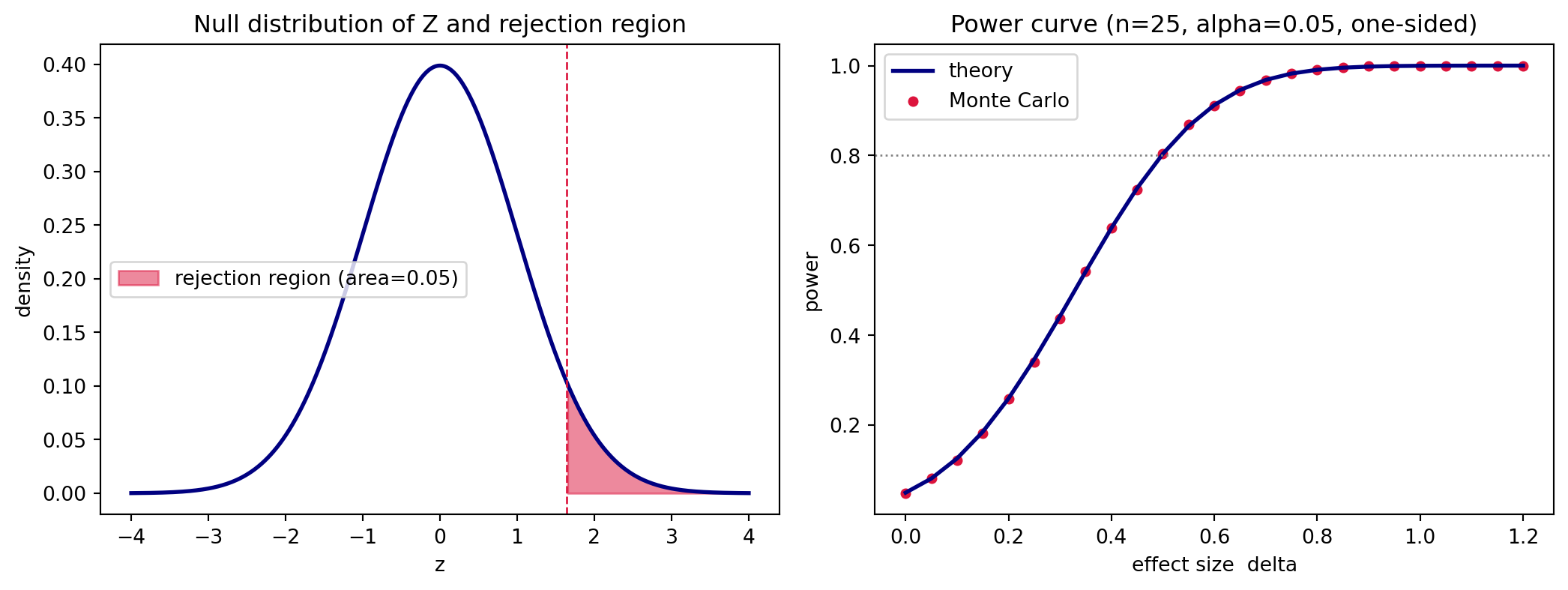
For example, to detect \(\delta = 0.5\) with \(80\%\) power at \(\alpha = 0.05\) one-sided, we have \(z_{0.95} \approx 1.645\) and \(z_{0.80} \approx 0.842\), giving \(n = ((1.645 + 0.842)/0.5)^2 \approx 24.7\), so \(25\) observations. The power curve in the code below plots this \(\Phi(\delta\sqrt{n} - z_{1-\alpha})\) relationship and overlays a Monte Carlo estimate.
38.5.3 5.2 Why power analysis matters before and after
A power analysis run before data collection answers the question: how many samples do I need to have, say, an eighty percent chance of detecting an effect of a given size at \(\alpha = 0.05\)? Skipping this step is how studies end up underpowered, unable to detect the very effects they were designed to find. Underpowered studies are doubly harmful: they miss real effects, and when they do produce a significant result by chance, that result is more likely to be an overstatement of the true effect, a phenomenon known as the winner’s curse or Type M (magnitude) error [3]. In machine learning, the analog is running a comparison on a test set too small to distinguish the models, then reporting whichever model happened to win as the better one.
38.6 6. Common Tests
38.6.1 6.1 The t-test
The \(t\)-test is the workhorse for comparing means. Its one-sample form, given above, tests whether a single sample mean differs from a hypothesized value. The two-sample form tests whether two groups have different means. When the two samples are independent, the statistic is
in the Welch formulation that does not assume equal variances, which is the safer default. The \(t\)-test assumes the data are drawn from approximately normal populations, though by the central limit theorem the test of means is fairly robust to non-normality once sample sizes are moderate.
A crucial variant for ML evaluation is the paired \(t\)-test. When two models are evaluated on the same test instances, the measurements are not independent: a hard example is hard for both models. By taking the per-instance difference \(d_i = a_i - b_i\) and running a one-sample test on the differences against zero, the paired test removes the instance-to-instance variability and is far more powerful than treating the two score sets as independent. Pairing is almost always the right structure when comparing models on a shared benchmark.
38.6.2 6.2 The chi-squared test
The chi-squared test addresses categorical data rather than means. In its goodness-of-fit form it asks whether observed counts in \(k\) categories match expected counts under a hypothesized distribution. In its test-of-independence form, applied to a contingency table, it asks whether two categorical variables are associated. The statistic compares observed counts \(O_i\) to expected counts \(E_i\),
\[\chi^2 = \sum_{i} \frac{(O_i - E_i)^2}{E_i},\]
which under the null follows a chi-squared distribution whose degrees of freedom depend on the table dimensions. For a contingency table with \(r\) rows and \(c\) columns, the degrees of freedom are \((r-1)(c-1)\). The approximation degrades when expected counts are small, conventionally below five, in which case an exact test such as Fisher’s exact test is preferred. For comparing two classifiers on the same test set, McNemar’s test, itself a chi-squared test on the discordant pairs where the models disagree, is the standard choice [4].
38.6.3 6.3 Nonparametric and resampling alternatives
When distributional assumptions are doubtful, rank-based tests such as the Mann-Whitney \(U\) and the Wilcoxon signed-rank test replace the \(t\)-test and require only ordinal structure. More flexibly still, permutation tests build the null distribution directly by repeatedly shuffling labels or signs and recomputing the statistic, making minimal assumptions and adapting naturally to the bespoke metrics common in ML, where there is often no closed-form sampling distribution for, say, an F1 score or a BLEU score.
38.7 7. The Multiple Comparisons Problem
38.7.1 7.1 How error inflates
Everything above concerns a single test with a single \(\alpha\). The moment we run many tests, the guarantee unravels. If we perform \(m\) independent tests, each at level \(\alpha\), and the null is true for all of them, the probability that at least one comes up significant by chance is
\[P(\text{at least one false positive}) = 1 - (1 - \alpha)^m.\]
For \(\alpha = 0.05\) and \(m = 20\) tests, this is \(1 - 0.95^{20} \approx 0.64\). With twenty comparisons we are more likely than not to find at least one spurious significant result. This is the multiple comparisons problem, and it is the statistical engine behind much irreproducible research. The probability of at least one false positive across a family of tests is called the family-wise error rate.
38.7.2 7.2 Corrections
The simplest remedy is the Bonferroni correction, which tests each hypothesis at the stricter level \(\alpha / m\), guaranteeing that the family-wise error rate stays below \(\alpha\). Bonferroni is conservative, sacrificing power, and many refinements exist, such as the Holm step-down procedure, which is uniformly more powerful while offering the same family-wise guarantee.
When the number of comparisons is very large, as in screening thousands of features, controlling the family-wise error rate is too strict and kills all power. The modern alternative is to control the false discovery rate, the expected proportion of false positives among the rejected hypotheses, using the Benjamini-Hochberg procedure [5]. Controlling the false discovery rate accepts some false positives in exchange for far greater sensitivity, which is the right trade-off when the goal is discovery rather than confirmation.
38.7.3 7.3 Researcher degrees of freedom
The multiple comparisons problem is not only about explicit tests. Every analytic choice, which metric to report, which outliers to drop, when to stop collecting data, constitutes an implicit comparison. These researcher degrees of freedom, exploited consciously or not, vastly inflate the true false positive rate, a practice known as p-hacking. The cleanest defense is to preregister the analysis plan, fixing the hypotheses and tests before seeing the data, so that the reported p-values mean what they claim to mean.
38.8 8. Hypothesis Testing in Machine Learning Model Comparison
38.8.1 8.1 The proper use
When we claim model \(A\) outperforms model \(B\), we are asserting that the observed gap in some metric is larger than the variability we would expect from chance alone. Making this rigorous requires identifying the sources of that variability. There are at least three: the finite test set, the randomness of training (initialization, data ordering, augmentation), and the randomness of data splits. A single accuracy number on a single test set, reported without any measure of variability, is not evidence of superiority; it is an anecdote.
The right practice depends on the setting. For comparing two models on one shared test set, the paired structure applies, and McNemar’s test or a paired test on per-example losses is appropriate. For comparing learning algorithms, where the randomness of training matters, multiple training runs with different seeds and cross-validation give the relevant variability, and corrected resampled tests account for the dependence that ordinary cross-validation folds induce [6]. For comparing many classifiers across many datasets, the recommended procedure is the Friedman test followed by a post-hoc Nemenyi test, a framework laid out in detail by Demsar [7].
38.8.2 8.2 The common abuses
The misuses are unfortunately routine. The most pervasive is reporting a single run with no confidence interval and no test, so that a difference of a few tenths of a percent on a benchmark is presented as a meaningful advance when it lies well within run-to-run noise. Reproductions of well-known results have repeatedly shown that hyperparameter tuning budget and random seed can swamp the claimed architectural gains [8].
A second abuse is the multiple comparisons problem in disguise. A leaderboard with hundreds of submissions evaluated against a fixed test set is running hundreds of implicit tests, and the top entry is selected precisely because it scored highest, the winner’s curse again. The reported test accuracy of the leaderboard champion is an optimistically biased estimate of its true performance, because the test set has been used, collectively, for model selection.
A third abuse is conflating statistical and practical significance. On a benchmark with a million test examples, almost any difference becomes statistically significant, so a significant p-value alone certifies nothing about whether the gap matters. The remedy is to report effect sizes and confidence intervals alongside, or instead of, p-values, so that readers can judge the magnitude of the improvement, not merely its detectability.
38.8.3 8.3 Practical guidance
A defensible model comparison reports more than a point estimate. It states the source of variability being accounted for, runs the appropriate paired or corrected test, corrects for multiple comparisons when several models or datasets are involved, distinguishes statistical from practical significance by reporting effect sizes and intervals, and ideally fixes the evaluation protocol in advance. None of this is exotic; it is the same discipline that the rest of empirical science has had to learn, applied to a field whose enormous sample sizes and rapid iteration make the failure modes especially easy to fall into. Treating hypothesis testing as a ritual to be performed produces the abuses; treating it as a tool for honest reasoning about uncertainty produces credible claims.
38.9 9. Simulating the Theory
The derivations above make two falsifiable claims: that the rejection region of a \(z\)-test traps exactly an \(\alpha\) fraction of the null distribution, and that power follows \(\Phi(\delta\sqrt{n} - z_{1-\alpha})\). The following sections check both claims by simulation across three languages. The Python version is executable and produces the figures and printed numbers; the Julia and Rust versions are illustrative ports of the same logic.
38.9.1 9.1 Python (executable)
Code
import numpy as npimport matplotlib.pyplot as pltfrom scipy import statsrng = np.random.default_rng(20260620)# --- Setup: one-sided z-test of H0: mu = 0, known sigma = 1 ---mu0, sigma, n, alpha =0.0, 1.0, 25, 0.05z_crit = stats.norm.ppf(1- alpha) # one-sided critical value ~ 1.645crit_xbar = mu0 + z_crit * sigma / np.sqrt(n)# --- 1. Empirical Type I error: simulate the null distribution ---n_sim =200_000xbar_null = rng.normal(mu0, sigma / np.sqrt(n), size=n_sim)z_null = (xbar_null - mu0) / (sigma / np.sqrt(n))emp_type1 = np.mean(z_null > z_crit)print(f"Nominal alpha : {alpha:.4f}")print(f"Empirical Type I error : {emp_type1:.4f}")# --- 2. p-values are Uniform(0,1) under H0 (two-sided) ---p_null =2* (1- stats.norm.cdf(np.abs(z_null)))print(f"Fraction of p <= 0.05 : {np.mean(p_null <=0.05):.4f} (expect ~0.05)")# --- 3. Power: theory vs Monte Carlo over a grid of effect sizes ---deltas = np.linspace(0.0, 1.2, 25)power_theory = stats.norm.cdf(deltas * np.sqrt(n) - z_crit)power_mc = np.empty_like(deltas)for i, d inenumerate(deltas): xbar_alt = rng.normal(mu0 + d * sigma, sigma / np.sqrt(n), size=20_000) power_mc[i] = np.mean(xbar_alt > crit_xbar)d_check =0.5print(f"Power at delta=0.5 (theory): "f"{stats.norm.cdf(d_check*np.sqrt(n)-z_crit):.4f}")# --- Plots: null distribution with rejection region, and power curve ---fig, (ax1, ax2) = plt.subplots(1, 2, figsize=(11, 4.2))grid = np.linspace(-4, 4, 400)ax1.plot(grid, stats.norm.pdf(grid), color="navy", lw=2)mask = grid > z_critax1.fill_between(grid[mask], stats.norm.pdf(grid[mask]), color="crimson", alpha=0.5, label=f"rejection region (area={alpha})")ax1.axvline(z_crit, color="crimson", ls="--", lw=1)ax1.set_title("Null distribution of Z and rejection region")ax1.set_xlabel("z"); ax1.set_ylabel("density"); ax1.legend()ax2.plot(deltas, power_theory, color="navy", lw=2, label="theory")ax2.scatter(deltas, power_mc, color="crimson", s=18, label="Monte Carlo")ax2.axhline(0.8, color="grey", ls=":", lw=1)ax2.set_title(f"Power curve (n={n}, alpha={alpha}, one-sided)")ax2.set_xlabel("effect size delta"); ax2.set_ylabel("power")ax2.legend()plt.tight_layout()plt.show()
Nominal alpha          : 0.0500
Empirical Type I error : 0.0497
Fraction of p <= 0.05  : 0.0501  (expect ~0.05)
Power at delta=0.5 (theory): 0.8038
The empirical Type I error lands on the nominal \(\alpha\), the null p-values are uniform so the same \(5\%\) fraction falls below the threshold, and the Monte Carlo power points trace the theoretical curve, confirming the derivation in section 5.1a.
38.9.2 9.2 Julia
usingDistributions, Statistics, Randomrng =MersenneTwister(20260620)mu0, sigma, n, alpha =0.0, 1.0, 25, 0.05z_crit =quantile(Normal(), 1- alpha)crit_xbar = mu0 + z_crit * sigma /sqrt(n)# Empirical Type I error from the simulated null distributionnsim =200_000xbar_null =rand(rng, Normal(mu0, sigma /sqrt(n)), nsim)z_null = (xbar_null .- mu0) ./ (sigma /sqrt(n))emp_type1 =mean(z_null .> z_crit)println("Empirical Type I error: ", round(emp_type1, digits=4))# Power: theory vs Monte Carlodeltas =range(0.0, 1.2, length=25)power_theory =cdf.(Normal(), deltas .*sqrt(n) .- z_crit)power_mc = [mean(rand(rng, Normal(mu0 + d*sigma, sigma/sqrt(n)), 20_000) .> crit_xbar) for d in deltas]println("Power at delta=0.5: ", round(cdf(Normal(), 0.5*sqrt(n) - z_crit), digits=4))
38.9.3 9.3 Rust
// Illustrative: requires the `statrs` and `rand` crates.usestatrs::distribution::{Normal, ContinuousCDF};userand::SeedableRng;userand_distr::{Distribution, Normal as RandNormal};fn main() {let (mu0, sigma, n, alpha) = (0.0_f64,1.0_f64,25.0_f64,0.05_f64);let std_normal =Normal::new(0.0,1.0).unwrap();let z_crit = std_normal.inverse_cdf(1.0- alpha);// ~1.645let crit_xbar = mu0 + z_crit * sigma / n.sqrt();letmut rng =rand::rngs::StdRng::seed_from_u64(20260620);let null_dist =RandNormal::new(mu0, sigma / n.sqrt()).unwrap();// Empirical Type I errorlet nsim =200_000;let hits = (0..nsim).filter(|_| null_dist.sample(&mut rng) > crit_xbar).count();println!("Empirical Type I error: {:.4}", hits asf64/ nsim asf64);// Theoretical power at delta = 0.5let delta =0.5_f64;let power = std_normal.cdf(delta * n.sqrt() - z_crit);println!("Power at delta=0.5: {:.4}", power);}
38.10 References
Neyman, J. and Pearson, E. S. (1933). On the Problem of the Most Efficient Tests of Statistical Hypotheses. Philosophical Transactions of the Royal Society of London A, 231, 289-337. https://doi.org/10.1098/rsta.1933.0009
Wasserstein, R. L. and Lazar, N. A. (2016). The ASA Statement on p-Values: Context, Process, and Purpose. The American Statistician, 70(2), 129-133. https://doi.org/10.1080/00031305.2016.1154108
Gelman, A. and Carlin, J. (2014). Beyond Power Calculations: Assessing Type S (Sign) and Type M (Magnitude) Errors. Perspectives on Psychological Science, 9(6), 641-651. https://doi.org/10.1177/1745691614551642
Dietterich, T. G. (1998). Approximate Statistical Tests for Comparing Supervised Classification Learning Algorithms. Neural Computation, 10(7), 1895-1923. https://doi.org/10.1162/089976698300017197
Benjamini, Y. and Hochberg, Y. (1995). Controlling the False Discovery Rate: A Practical and Powerful Approach to Multiple Testing. Journal of the Royal Statistical Society: Series B, 57(1), 289-300. https://doi.org/10.1111/j.2517-6161.1995.tb02031.x
Nadeau, C. and Bengio, Y. (2003). Inference for the Generalization Error. Machine Learning, 52(3), 239-281. https://doi.org/10.1023/A:1024068626366
Demsar, J. (2006). Statistical Comparisons of Classifiers over Multiple Data Sets. Journal of Machine Learning Research, 7, 1-30. https://www.jmlr.org/papers/v7/demsar06a.html
Henderson, P., Islam, R., Bachman, P., Pineau, J., Precup, D. and Meger, D. (2018). Deep Reinforcement Learning that Matters. Proceedings of the AAAI Conference on Artificial Intelligence, 32(1). https://doi.org/10.1609/aaai.v32i1.11694
Source Code
# Hypothesis TestingHypothesis testing is the formal machinery that statistics offers for deciding whether a pattern in data reflects a real effect or could plausibly be the product of chance alone. For practitioners of machine learning, this machinery is both indispensable and dangerous. It is indispensable because almost every claim we make about a model, that one architecture beats another, that a feature improves accuracy, that a deployment shift is real and not noise, is at bottom a statistical claim. It is dangerous because the formalism is widely misunderstood, and the misunderstandings are precisely the ones that lead to overconfident, irreproducible conclusions. This chapter develops the logic of hypothesis testing carefully, defines its core quantities, catalogs the most common tests, and then turns to how the framework is applied and abused when we compare machine learning models.## 1. The Logic of Null and Alternative Hypotheses### 1.1 The two hypothesesA hypothesis test begins by partitioning the possible states of the world into two complementary claims. The null hypothesis, written $H_0$, is a specific statement that there is no effect, no difference, or no relationship. The alternative hypothesis, written $H_1$ or $H_a$, is the claim we entertain if the null is found implausible. The asymmetry between them is deliberate and important. The null is the default, the position of skepticism that we hold until the data force us to abandon it. The test is constructed so that we either reject $H_0$ in favor of $H_1$, or fail to reject $H_0$. We never accept $H_0$ as proven true.Concretely, suppose we measure the difference in mean accuracy between two classifiers across a set of test instances. A natural null is that the true mean difference is zero,$$H_0: \mu_A - \mu_B = 0,$$against the two-sided alternative$$H_1: \mu_A - \mu_B \neq 0.$$If we had a directional prior belief, for instance that model $A$ can only help, we might instead use the one-sided alternative $H_1: \mu_A - \mu_B > 0$. The choice of one-sided versus two-sided must be made before seeing the data, because switching after the fact silently doubles the effective error rate.### 1.2 Why we reason from the nullThe reason we frame everything around a null of no effect is that the null is usually a sharp, fully specified hypothesis. Under $H_0$ we can often compute, exactly or approximately, the distribution of any statistic we choose to measure. The alternative, by contrast, is typically composite: it covers a whole range of possible effect sizes, and we cannot compute a single sampling distribution for it without committing to one specific value. Hypothesis testing therefore proceeds by assuming the null is true, asking how surprising the observed data would be under that assumption, and rejecting the null only when the data are surprising enough.### 1.3 The Neyman-Pearson frameworkTwo distinct philosophies underlie modern testing, and conflating them is the root of much confusion. Fisher treated the p-value as a continuous measure of evidence against the null, to be weighed by judgment. Neyman and Pearson recast testing as a decision procedure with controlled long-run error rates [1]. In their formulation we fix in advance a significance level $\alpha$, partition the sample space into a rejection region $R$ and its complement, and adopt the rule: reject $H_0$ if and only if the data fall in $R$. The region is chosen so that the false positive rate is controlled,$$P(\text{data} \in R \mid H_0) \leq \alpha,$$and, subject to that constraint, the power $P(\text{data} \in R \mid H_1)$ is made as large as possible.The cornerstone result is the Neyman-Pearson lemma. For testing a simple null $H_0: \theta = \theta_0$ against a simple alternative $H_1: \theta = \theta_1$, the most powerful test of level $\alpha$ rejects when the likelihood ratio exceeds a threshold,$$\Lambda(x) = \frac{L(\theta_1 \mid x)}{L(\theta_0 \mid x)} \geq k,$$with $k$ chosen so that $P(\Lambda \geq k \mid H_0) = \alpha$. No other test with the same Type I error rate achieves higher power. This lemma is why so many standard tests, the $z$-test and $t$-test among them, take the form of comparing a statistic against a critical threshold: they are likelihood-ratio tests in disguise, and their rejection regions are optimal. The practical reading is that a test is a fixed rule chosen before the data arrive, and its quality is judged by two numbers, its size $\alpha$ and its power, not by the particular p-value it happens to return on one dataset.## 2. Test Statistics and Their Sampling Distributions### 2.1 From data to a single numberA test statistic is a function of the data that summarizes the evidence relevant to the hypotheses into a single number, and whose distribution under $H_0$ is known. The art of designing a test lies in choosing a statistic that is sensitive to the alternative, large when $H_1$ holds, yet has a tractable distribution when $H_0$ holds.The canonical example is the one-sample $t$ statistic. Given $n$ observations $x_1, \dots, x_n$ with sample mean $\bar{x}$ and sample standard deviation $s$, and a null value $\mu_0$, we form$$t = \frac{\bar{x} - \mu_0}{s / \sqrt{n}}.$$The numerator measures how far the observed mean sits from the null value, and the denominator, the standard error of the mean, rescales that distance into units of sampling variability. If the null holds and the data are approximately normal, this statistic follows a Student $t$ distribution with $n - 1$ degrees of freedom.### 2.2 The sampling distributionThe key conceptual object is the sampling distribution: the distribution of the test statistic across hypothetical repetitions of the experiment, assuming $H_0$ is true. We almost never observe this distribution directly. Instead we derive it from theory, as with the $t$ and chi-squared families, or we approximate it through resampling methods such as the permutation test and the bootstrap. Once we know the sampling distribution, the observed value of the statistic can be placed on it, and we can ask how far into the tail it falls.The simplest null distribution to reason about is that of the $z$-statistic. Suppose we observe $n$ independent draws from a population with unknown mean $\mu$ but known standard deviation $\sigma$, and we test $H_0: \mu = \mu_0$. The standardized statistic$$Z = \frac{\bar{X} - \mu_0}{\sigma / \sqrt{n}}$$has, under $H_0$, exactly the standard normal distribution $Z \sim \mathcal{N}(0, 1)$, because $\bar{X} \sim \mathcal{N}(\mu_0, \sigma^2/n)$ and subtracting the mean and dividing by the standard deviation of a normal random variable produces a standard normal. When $\sigma$ is unknown and replaced by the sample standard deviation $s$, the extra estimation noise in the denominator broadens the tails and the statistic follows a Student $t$ distribution with $n-1$ degrees of freedom, converging to the normal as $n$ grows. This pair, the $z$ when the scale is known and the $t$ when it is estimated, is the backbone of the worked derivations below.## 3. P-values and Their Correct Interpretation### 3.1 DefinitionThe p-value is the probability, computed under the assumption that $H_0$ is true, of obtaining a test statistic at least as extreme as the one actually observed. Writing $T$ for the random test statistic and $t_{\text{obs}}$ for the observed value, a two-sided p-value is$$p = P\big(|T| \geq |t_{\text{obs}}| \;\big|\; H_0\big).$$A small p-value means the observed data are unlikely under the null, which we take as evidence against the null. The conventional threshold $\alpha = 0.05$ is a social convention inherited from Fisher, not a law of nature, and there is nothing magical about it.### 3.1a Deriving a p-value for a simple caseConsider the cleanest possible setting: a known-variance $z$-test of $H_0: \mu = \mu_0$ against the two-sided alternative $H_1: \mu \neq \mu_0$. We observe the statistic $z_{\text{obs}} = (\bar{x} - \mu_0)/(\sigma/\sqrt{n})$. Under $H_0$ the random version $Z$ is standard normal, so the two-sided p-value is the probability that a standard normal lands at least as far from zero as $z_{\text{obs}}$,$$p = P\big(|Z| \geq |z_{\text{obs}}|\big) = 2\big(1 - \Phi(|z_{\text{obs}}|)\big),$$where $\Phi$ is the standard normal cumulative distribution function. The factor of two accounts for the two tails of the symmetric distribution. For a concrete number, suppose $z_{\text{obs}} = 1.96$. Then $\Phi(1.96) \approx 0.975$, so $p \approx 2(1 - 0.975) = 0.05$. This is exactly why $1.96$ is the familiar critical value for a two-sided test at $\alpha = 0.05$: it is the point beyond which each tail holds $2.5\%$ of the mass. A crucial structural fact follows from this construction. Under $H_0$ the p-value is itself a random variable, and because $p = 2(1 - \Phi(|Z|))$ is a monotone transformation of a continuous statistic, it is uniformly distributed on $[0, 1]$. That uniformity is the engine behind the whole framework: rejecting whenever $p \leq \alpha$ then yields $P(p \leq \alpha \mid H_0) = \alpha$, so the test has exactly the intended size. The simulation below checks this property empirically.### 3.2 What the p-value is notThe p-value is one of the most misinterpreted quantities in all of science, and the American Statistical Association issued a formal statement in 2016 to combat the confusion [2]. Several errors are worth naming explicitly.The p-value is not the probability that the null hypothesis is true. That would be $P(H_0 \mid \text{data})$, a posterior quantity, whereas the p-value is $P(\text{data or more extreme} \mid H_0)$, a likelihood-like quantity computed in the opposite direction. Confusing the two is the transposed conditional fallacy, and the two probabilities can differ enormously.The p-value is not the probability that the result is due to chance. The result either reflects a real effect or it does not; the p-value quantifies how compatible the data are with the chance-only model, not the probability that chance is the explanation.A non-significant p-value, say $p = 0.4$, does not establish that $H_0$ is true. Absence of evidence is not evidence of absence. It may simply mean the study had too little power to detect a real effect. Finally, the p-value says nothing on its own about the size or practical importance of an effect. With a large enough sample, a trivially small and meaningless difference can produce an arbitrarily small p-value. Statistical significance and practical significance are different things, and conflating them is a recurring source of error in large-scale ML evaluation, where sample sizes are huge.## 4. Type I and Type II Errors### 4.1 The two ways to be wrongBecause a test reaches a verdict on the basis of finite, noisy data, it can be wrong in two distinct ways. A Type I error occurs when we reject a null hypothesis that is in fact true: a false positive, a claim of an effect that is not there. A Type II error occurs when we fail to reject a null that is in fact false: a false negative, a missed real effect. The structure is summarized below.|| $H_0$ true | $H_0$ false ||---|---|---|| Reject $H_0$ | Type I error (prob. $\alpha$) | Correct (prob. $1 - \beta$) || Fail to reject $H_0$ | Correct (prob. $1 - \alpha$) | Type II error (prob. $\beta$) |### 4.2 The significance level and the trade-offThe significance level $\alpha$ is the probability of a Type I error that we are willing to tolerate, fixed in advance. By choosing $\alpha = 0.05$ we are saying that, when the null is true, we will wrongly reject it at most five percent of the time across repeated experiments. The probability of a Type II error is denoted $\beta$.These two error rates are in tension. Holding the sample size and the true effect fixed, making the test more conservative, lowering $\alpha$, makes it harder to reject the null and therefore raises $\beta$. We cannot drive both errors to zero simultaneously with finite data. The only way to reduce both at once is to collect more information, which is why sample size is the lever that matters most. The asymmetry in how we treat the two errors reflects a value judgment: in the classical framework we regard a false positive as more costly than a false negative, and we control $\alpha$ tightly while letting $\beta$ float.## 5. Statistical Power### 5.1 Definition and determinantsThe power of a test is the probability that it correctly rejects a false null hypothesis,$$\text{power} = 1 - \beta = P(\text{reject } H_0 \mid H_1 \text{ true}).$$Power is the test's sensitivity, its ability to detect a real effect when one exists. Four quantities are bound together in a single relationship, so that fixing any three determines the fourth: the significance level $\alpha$, the true effect size, the sample size $n$, and the power $1 - \beta$. Power increases as the effect size grows, as the sample size grows, as the noise shrinks, and as we relax $\alpha$.For a comparison of two means, the relevant effect size is often Cohen's $d$, the difference in means divided by the pooled standard deviation,$$d = \frac{\mu_A - \mu_B}{\sigma}.$$A common convention takes $d \approx 0.2$ as small, $0.5$ as medium, and $0.8$ as large, though these labels should be treated as rough anchors rather than universal truths.### 5.1a Deriving the power of a z-testPower is not a vague notion; for the $z$-test it has a closed form, and deriving it shows exactly how the four quantities lock together. Take the one-sided test of $H_0: \mu = \mu_0$ against $H_1: \mu = \mu_1$ with $\mu_1 > \mu_0$, known variance $\sigma^2$, and sample size $n$. We reject when $Z = (\bar{X} - \mu_0)/(\sigma/\sqrt{n})$ exceeds the critical value $z_{1-\alpha}$, the $(1-\alpha)$ quantile of the standard normal. Equivalently, we reject when$$\bar{X} > \mu_0 + z_{1-\alpha}\,\frac{\sigma}{\sqrt{n}}.$$Power is the probability of this event computed under the alternative, where $\bar{X} \sim \mathcal{N}(\mu_1, \sigma^2/n)$. Standardizing with respect to $\mu_1$ rather than $\mu_0$,$$\text{power} = P\!\left(\bar{X} > \mu_0 + z_{1-\alpha}\frac{\sigma}{\sqrt{n}} \;\Big|\; \mu = \mu_1\right) = P\!\left(\frac{\bar{X} - \mu_1}{\sigma/\sqrt{n}} > z_{1-\alpha} - \frac{\mu_1 - \mu_0}{\sigma/\sqrt{n}}\right).$$The quantity inside is again standard normal under $H_1$, so writing the effect size as $\delta = (\mu_1 - \mu_0)/\sigma$ and using $1 - \Phi(x) = \Phi(-x)$,$$\text{power} = 1 - \Phi\!\left(z_{1-\alpha} - \delta\sqrt{n}\right) = \Phi\!\left(\delta\sqrt{n} - z_{1-\alpha}\right).$$This single formula contains every qualitative claim made earlier. Power rises with the effect size $\delta$, rises with the sample size $n$ through the $\sqrt{n}$ term, and rises as we relax $\alpha$ (which lowers $z_{1-\alpha}$). Inverting it gives the sample size needed for a target power $1 - \beta$: setting $\delta\sqrt{n} - z_{1-\alpha} = z_{1-\beta}$ yields$$n = \left(\frac{z_{1-\alpha} + z_{1-\beta}}{\delta}\right)^{2}.$$For example, to detect $\delta = 0.5$ with $80\%$ power at $\alpha = 0.05$ one-sided, we have $z_{0.95} \approx 1.645$ and $z_{0.80} \approx 0.842$, giving $n = ((1.645 + 0.842)/0.5)^2 \approx 24.7$, so $25$ observations. The power curve in the code below plots this $\Phi(\delta\sqrt{n} - z_{1-\alpha})$ relationship and overlays a Monte Carlo estimate.### 5.2 Why power analysis matters before and afterA power analysis run before data collection answers the question: how many samples do I need to have, say, an eighty percent chance of detecting an effect of a given size at $\alpha = 0.05$? Skipping this step is how studies end up underpowered, unable to detect the very effects they were designed to find. Underpowered studies are doubly harmful: they miss real effects, and when they do produce a significant result by chance, that result is more likely to be an overstatement of the true effect, a phenomenon known as the winner's curse or Type M (magnitude) error [3]. In machine learning, the analog is running a comparison on a test set too small to distinguish the models, then reporting whichever model happened to win as the better one.## 6. Common Tests### 6.1 The t-testThe $t$-test is the workhorse for comparing means. Its one-sample form, given above, tests whether a single sample mean differs from a hypothesized value. The two-sample form tests whether two groups have different means. When the two samples are independent, the statistic is$$t = \frac{\bar{x}_A - \bar{x}_B}{\sqrt{\dfrac{s_A^2}{n_A} + \dfrac{s_B^2}{n_B}}},$$in the Welch formulation that does not assume equal variances, which is the safer default. The $t$-test assumes the data are drawn from approximately normal populations, though by the central limit theorem the test of means is fairly robust to non-normality once sample sizes are moderate.A crucial variant for ML evaluation is the paired $t$-test. When two models are evaluated on the same test instances, the measurements are not independent: a hard example is hard for both models. By taking the per-instance difference $d_i = a_i - b_i$ and running a one-sample test on the differences against zero, the paired test removes the instance-to-instance variability and is far more powerful than treating the two score sets as independent. Pairing is almost always the right structure when comparing models on a shared benchmark.### 6.2 The chi-squared testThe chi-squared test addresses categorical data rather than means. In its goodness-of-fit form it asks whether observed counts in $k$ categories match expected counts under a hypothesized distribution. In its test-of-independence form, applied to a contingency table, it asks whether two categorical variables are associated. The statistic compares observed counts $O_i$ to expected counts $E_i$,$$\chi^2 = \sum_{i} \frac{(O_i - E_i)^2}{E_i},$$which under the null follows a chi-squared distribution whose degrees of freedom depend on the table dimensions. For a contingency table with $r$ rows and $c$ columns, the degrees of freedom are $(r-1)(c-1)$. The approximation degrades when expected counts are small, conventionally below five, in which case an exact test such as Fisher's exact test is preferred. For comparing two classifiers on the same test set, McNemar's test, itself a chi-squared test on the discordant pairs where the models disagree, is the standard choice [4].### 6.3 Nonparametric and resampling alternativesWhen distributional assumptions are doubtful, rank-based tests such as the Mann-Whitney $U$ and the Wilcoxon signed-rank test replace the $t$-test and require only ordinal structure. More flexibly still, permutation tests build the null distribution directly by repeatedly shuffling labels or signs and recomputing the statistic, making minimal assumptions and adapting naturally to the bespoke metrics common in ML, where there is often no closed-form sampling distribution for, say, an F1 score or a BLEU score.## 7. The Multiple Comparisons Problem### 7.1 How error inflatesEverything above concerns a single test with a single $\alpha$. The moment we run many tests, the guarantee unravels. If we perform $m$ independent tests, each at level $\alpha$, and the null is true for all of them, the probability that at least one comes up significant by chance is$$P(\text{at least one false positive}) = 1 - (1 - \alpha)^m.$$For $\alpha = 0.05$ and $m = 20$ tests, this is $1 - 0.95^{20} \approx 0.64$. With twenty comparisons we are more likely than not to find at least one spurious significant result. This is the multiple comparisons problem, and it is the statistical engine behind much irreproducible research. The probability of at least one false positive across a family of tests is called the family-wise error rate.### 7.2 CorrectionsThe simplest remedy is the Bonferroni correction, which tests each hypothesis at the stricter level $\alpha / m$, guaranteeing that the family-wise error rate stays below $\alpha$. Bonferroni is conservative, sacrificing power, and many refinements exist, such as the Holm step-down procedure, which is uniformly more powerful while offering the same family-wise guarantee.When the number of comparisons is very large, as in screening thousands of features, controlling the family-wise error rate is too strict and kills all power. The modern alternative is to control the false discovery rate, the expected proportion of false positives among the rejected hypotheses, using the Benjamini-Hochberg procedure [5]. Controlling the false discovery rate accepts some false positives in exchange for far greater sensitivity, which is the right trade-off when the goal is discovery rather than confirmation.### 7.3 Researcher degrees of freedomThe multiple comparisons problem is not only about explicit tests. Every analytic choice, which metric to report, which outliers to drop, when to stop collecting data, constitutes an implicit comparison. These researcher degrees of freedom, exploited consciously or not, vastly inflate the true false positive rate, a practice known as p-hacking. The cleanest defense is to preregister the analysis plan, fixing the hypotheses and tests before seeing the data, so that the reported p-values mean what they claim to mean.## 8. Hypothesis Testing in Machine Learning Model Comparison### 8.1 The proper useWhen we claim model $A$ outperforms model $B$, we are asserting that the observed gap in some metric is larger than the variability we would expect from chance alone. Making this rigorous requires identifying the sources of that variability. There are at least three: the finite test set, the randomness of training (initialization, data ordering, augmentation), and the randomness of data splits. A single accuracy number on a single test set, reported without any measure of variability, is not evidence of superiority; it is an anecdote.The right practice depends on the setting. For comparing two models on one shared test set, the paired structure applies, and McNemar's test or a paired test on per-example losses is appropriate. For comparing learning algorithms, where the randomness of training matters, multiple training runs with different seeds and cross-validation give the relevant variability, and corrected resampled tests account for the dependence that ordinary cross-validation folds induce [6]. For comparing many classifiers across many datasets, the recommended procedure is the Friedman test followed by a post-hoc Nemenyi test, a framework laid out in detail by Demsar [7].### 8.2 The common abusesThe misuses are unfortunately routine. The most pervasive is reporting a single run with no confidence interval and no test, so that a difference of a few tenths of a percent on a benchmark is presented as a meaningful advance when it lies well within run-to-run noise. Reproductions of well-known results have repeatedly shown that hyperparameter tuning budget and random seed can swamp the claimed architectural gains [8].A second abuse is the multiple comparisons problem in disguise. A leaderboard with hundreds of submissions evaluated against a fixed test set is running hundreds of implicit tests, and the top entry is selected precisely because it scored highest, the winner's curse again. The reported test accuracy of the leaderboard champion is an optimistically biased estimate of its true performance, because the test set has been used, collectively, for model selection.A third abuse is conflating statistical and practical significance. On a benchmark with a million test examples, almost any difference becomes statistically significant, so a significant p-value alone certifies nothing about whether the gap matters. The remedy is to report effect sizes and confidence intervals alongside, or instead of, p-values, so that readers can judge the magnitude of the improvement, not merely its detectability.### 8.3 Practical guidanceA defensible model comparison reports more than a point estimate. It states the source of variability being accounted for, runs the appropriate paired or corrected test, corrects for multiple comparisons when several models or datasets are involved, distinguishes statistical from practical significance by reporting effect sizes and intervals, and ideally fixes the evaluation protocol in advance. None of this is exotic; it is the same discipline that the rest of empirical science has had to learn, applied to a field whose enormous sample sizes and rapid iteration make the failure modes especially easy to fall into. Treating hypothesis testing as a ritual to be performed produces the abuses; treating it as a tool for honest reasoning about uncertainty produces credible claims.## 9. Simulating the TheoryThe derivations above make two falsifiable claims: that the rejection region of a $z$-test traps exactly an $\alpha$ fraction of the null distribution, and that power follows $\Phi(\delta\sqrt{n} - z_{1-\alpha})$. The following sections check both claims by simulation across three languages. The Python version is executable and produces the figures and printed numbers; the Julia and Rust versions are illustrative ports of the same logic.### 9.1 Python (executable)```{python}import numpy as npimport matplotlib.pyplot as pltfrom scipy import statsrng = np.random.default_rng(20260620)# --- Setup: one-sided z-test of H0: mu = 0, known sigma = 1 ---mu0, sigma, n, alpha =0.0, 1.0, 25, 0.05z_crit = stats.norm.ppf(1- alpha) # one-sided critical value ~ 1.645crit_xbar = mu0 + z_crit * sigma / np.sqrt(n)# --- 1. Empirical Type I error: simulate the null distribution ---n_sim =200_000xbar_null = rng.normal(mu0, sigma / np.sqrt(n), size=n_sim)z_null = (xbar_null - mu0) / (sigma / np.sqrt(n))emp_type1 = np.mean(z_null > z_crit)print(f"Nominal alpha : {alpha:.4f}")print(f"Empirical Type I error : {emp_type1:.4f}")# --- 2. p-values are Uniform(0,1) under H0 (two-sided) ---p_null =2* (1- stats.norm.cdf(np.abs(z_null)))print(f"Fraction of p <= 0.05 : {np.mean(p_null <=0.05):.4f} (expect ~0.05)")# --- 3. Power: theory vs Monte Carlo over a grid of effect sizes ---deltas = np.linspace(0.0, 1.2, 25)power_theory = stats.norm.cdf(deltas * np.sqrt(n) - z_crit)power_mc = np.empty_like(deltas)for i, d inenumerate(deltas): xbar_alt = rng.normal(mu0 + d * sigma, sigma / np.sqrt(n), size=20_000) power_mc[i] = np.mean(xbar_alt > crit_xbar)d_check =0.5print(f"Power at delta=0.5 (theory): "f"{stats.norm.cdf(d_check*np.sqrt(n)-z_crit):.4f}")# --- Plots: null distribution with rejection region, and power curve ---fig, (ax1, ax2) = plt.subplots(1, 2, figsize=(11, 4.2))grid = np.linspace(-4, 4, 400)ax1.plot(grid, stats.norm.pdf(grid), color="navy", lw=2)mask = grid > z_critax1.fill_between(grid[mask], stats.norm.pdf(grid[mask]), color="crimson", alpha=0.5, label=f"rejection region (area={alpha})")ax1.axvline(z_crit, color="crimson", ls="--", lw=1)ax1.set_title("Null distribution of Z and rejection region")ax1.set_xlabel("z"); ax1.set_ylabel("density"); ax1.legend()ax2.plot(deltas, power_theory, color="navy", lw=2, label="theory")ax2.scatter(deltas, power_mc, color="crimson", s=18, label="Monte Carlo")ax2.axhline(0.8, color="grey", ls=":", lw=1)ax2.set_title(f"Power curve (n={n}, alpha={alpha}, one-sided)")ax2.set_xlabel("effect size delta"); ax2.set_ylabel("power")ax2.legend()plt.tight_layout()plt.show()```The empirical Type I error lands on the nominal $\alpha$, the null p-values are uniform so the same $5\%$ fraction falls below the threshold, and the Monte Carlo power points trace the theoretical curve, confirming the derivation in section 5.1a.### 9.2 Julia```juliausingDistributions, Statistics, Randomrng =MersenneTwister(20260620)mu0, sigma, n, alpha =0.0, 1.0, 25, 0.05z_crit =quantile(Normal(), 1- alpha)crit_xbar = mu0 + z_crit * sigma /sqrt(n)# Empirical Type I error from the simulated null distributionnsim =200_000xbar_null =rand(rng, Normal(mu0, sigma /sqrt(n)), nsim)z_null = (xbar_null .- mu0) ./ (sigma /sqrt(n))emp_type1 =mean(z_null .> z_crit)println("Empirical Type I error: ", round(emp_type1, digits=4))# Power: theory vs Monte Carlodeltas =range(0.0, 1.2, length=25)power_theory =cdf.(Normal(), deltas .*sqrt(n) .- z_crit)power_mc = [mean(rand(rng, Normal(mu0 + d*sigma, sigma/sqrt(n)), 20_000) .> crit_xbar) for d in deltas]println("Power at delta=0.5: ", round(cdf(Normal(), 0.5*sqrt(n) - z_crit), digits=4))```### 9.3 Rust```rust// Illustrative: requires the `statrs` and `rand` crates.use statrs::distribution::{Normal, ContinuousCDF};use rand::SeedableRng;use rand_distr::{Distribution, Normal as RandNormal};fn main() {let (mu0, sigma, n, alpha) = (0.0_f64, 1.0_f64, 25.0_f64, 0.05_f64); let std_normal = Normal::new(0.0, 1.0).unwrap(); let z_crit =std_normal.inverse_cdf(1.0- alpha); //~1.645 let crit_xbar = mu0 + z_crit * sigma /n.sqrt(); let mut rng = rand::rngs::StdRng::seed_from_u64(20260620); let null_dist = RandNormal::new(mu0, sigma /n.sqrt()).unwrap();// Empirical Type I error let nsim =200_000; let hits = (0..nsim).filter(|_|null_dist.sample(&mut rng) > crit_xbar).count(); println!("Empirical Type I error: {:.4}", hits as f64 / nsim as f64);// Theoretical power at delta =0.5 let delta =0.5_f64; let power =std_normal.cdf(delta *n.sqrt() - z_crit); println!("Power at delta=0.5: {:.4}", power);}```## References1. Neyman, J. and Pearson, E. S. (1933). On the Problem of the Most Efficient Tests of Statistical Hypotheses. Philosophical Transactions of the Royal Society of London A, 231, 289-337. https://doi.org/10.1098/rsta.1933.00092. Wasserstein, R. L. and Lazar, N. A. (2016). The ASA Statement on p-Values: Context, Process, and Purpose. The American Statistician, 70(2), 129-133. https://doi.org/10.1080/00031305.2016.11541083. Gelman, A. and Carlin, J. (2014). Beyond Power Calculations: Assessing Type S (Sign) and Type M (Magnitude) Errors. Perspectives on Psychological Science, 9(6), 641-651. https://doi.org/10.1177/17456916145516424. Dietterich, T. G. (1998). Approximate Statistical Tests for Comparing Supervised Classification Learning Algorithms. Neural Computation, 10(7), 1895-1923. https://doi.org/10.1162/0899766983000171975. Benjamini, Y. and Hochberg, Y. (1995). Controlling the False Discovery Rate: A Practical and Powerful Approach to Multiple Testing. Journal of the Royal Statistical Society: Series B, 57(1), 289-300. https://doi.org/10.1111/j.2517-6161.1995.tb02031.x6. Nadeau, C. and Bengio, Y. (2003). Inference for the Generalization Error. Machine Learning, 52(3), 239-281. https://doi.org/10.1023/A:10240686263667. Demsar, J. (2006). Statistical Comparisons of Classifiers over Multiple Data Sets. Journal of Machine Learning Research, 7, 1-30. https://www.jmlr.org/papers/v7/demsar06a.html8. Henderson, P., Islam, R., Bachman, P., Pineau, J., Precup, D. and Meger, D. (2018). Deep Reinforcement Learning that Matters. Proceedings of the AAAI Conference on Artificial Intelligence, 32(1). https://doi.org/10.1609/aaai.v32i1.11694