Stochastic gradient descent reduces a loss function by stepping in the direction of the negative gradient, but a single global learning rate rarely suits every parameter at once. In deep networks the curvature of the loss surface varies wildly across coordinates, gradients arrive with very different magnitudes, and the scale of those magnitudes drifts as training proceeds. Adam, short for adaptive moment estimation, addresses these difficulties by maintaining running estimates of the gradient and its squared magnitude, then using those estimates to scale each parameter update individually. Introduced by Kingma and Ba in 2015, Adam has become the default optimizer for a large fraction of deep learning practice, from transformers to generative models. This chapter develops Adam from its two parent algorithms, derives its moment estimates and the bias correction that makes them trustworthy early in training, states the full update rule, and closes with the practical defaults that have proven durable.
201.1 1. Background: Two Ideas Adam Inherits
Adam is best understood as the fusion of two earlier refinements of plain stochastic gradient descent. Each solves a distinct problem, and Adam keeps both solutions.
201.1.1 1.1 Momentum
Plain SGD updates parameters \(\theta\) by
\[
\theta_t = \theta_{t-1} - \alpha \, g_t,
\]
where \(g_t = \nabla_\theta f_t(\theta_{t-1})\) is the stochastic gradient of the minibatch loss at step \(t\) and \(\alpha\) is the learning rate. When the loss surface forms a long narrow ravine, this update oscillates across the steep walls while crawling slowly along the gentle floor. Momentum damps the oscillation by accumulating an exponentially weighted average of past gradients,
with \(\beta\) typically near \(0.9\). The averaged direction \(v_t\) reinforces components that point consistently the same way and cancels components that flip sign, so the trajectory accelerates along the ravine floor. This is the first moment idea: track the mean of the gradient.
201.1.2 1.2 RMSProp
A separate problem is that a fixed \(\alpha\) is too large for parameters with big gradients and too small for parameters with tiny gradients. RMSProp, proposed by Tieleman and Hinton, adapts the step size per coordinate by dividing the gradient by the square root of a running average of squared gradients,
where \(g_t^2\) denotes the elementwise square. Coordinates whose gradients have been large get a small effective learning rate, and coordinates whose gradients have been small get a large one. This normalization keeps the update roughly the same scale across parameters regardless of raw gradient magnitude. This is the second moment idea: track the mean of the squared gradient.
Adam combines momentum, which smooths the direction, with RMSProp, which rescales the magnitude per coordinate.
201.2 2. The First and Second Moment Estimates
Adam maintains two exponential moving averages, one for the gradient and one for its elementwise square. At step \(t\), given the gradient \(g_t\), the updates are
initialized at \(m_0 = 0\) and \(v_0 = 0\). The vector \(m_t\) estimates the first moment of the gradient, its mean, and \(v_t\) estimates the second raw moment, the mean of the squared gradient. The decay rates \(\beta_1, \beta_2 \in [0, 1)\) control how much history each average retains. A larger \(\beta\) gives a longer memory and a smoother estimate; a smaller \(\beta\) tracks recent gradients more responsively.
It is useful to see why \(m_t\) and \(v_t\) deserve the name moment estimates. Unrolling the recursion for the first moment gives a weighted sum of all past gradients,
The weights \((1 - \beta_1)\beta_1^{\,t-i}\) are nonnegative and, in the limit of many steps, sum to one. So \(m_t\) is a properly normalized weighted average of the gradient history, with the most recent gradients weighted most heavily and older gradients decaying geometrically. The identical argument applies to \(v_t\) with \(\beta_2\) and \(g_i^2\). Both quantities are therefore exponentially weighted estimates of the corresponding moments of the gradient distribution under the minibatch sampling.
201.3 3. Why Bias Correction Is Needed
The moving averages are initialized to zero, and that initialization introduces a systematic bias toward zero in the early steps. Consider the first moment at step one:
If \(\beta_1 = 0.9\), then \(m_1 = 0.1\, g_1\), only a tenth of the gradient. The estimate is badly shrunk toward zero precisely because there is no accumulated history to fill the average. The same shrinkage afflicts \(v_t\) even more severely, since \(\beta_2\) is usually closer to one.
We can quantify the bias exactly. Suppose the gradients \(g_i\) are drawn so that the second moment is approximately stationary, \(\mathbb{E}[g_i^2] = \mathbb{E}[g_t^2]\) over the relevant window. Taking the expectation of the unrolled second moment estimate,
The factor \(1 - \beta_2^{\,t}\) is the source of the bias. Early in training it is much less than one, so \(v_t\) underestimates the true second moment. As \(t\) grows, \(\beta_2^{\,t} \to 0\) and the factor approaches one, so the bias vanishes asymptotically. The analogous result holds for the first moment, \(\mathbb{E}[m_t] = \mathbb{E}[g_t]\,(1 - \beta_1^{\,t})\).
The remedy follows immediately. Dividing each estimate by its bias factor produces a corrected estimate whose expectation matches the true moment:
These corrected quantities \(\hat{m}_t\) and \(\hat{v}_t\) are what Adam actually uses in its step. The correction matters most in the opening hundreds or thousands of iterations; once \(\beta_1^{\,t}\) and \(\beta_2^{\,t}\) have decayed to negligible values, the corrected and uncorrected estimates coincide. Without it, the first updates would be artificially tiny and the per-coordinate scaling would be distorted, which can slow or destabilize the start of training.
The plot below traces the two bias-correction denominators across the first thousand steps. The first moment, with \(\beta_1 = 0.9\), recovers in a few dozen steps, while the second moment, with \(\beta_2 = 0.999\), takes far longer, which is exactly why its early estimate is the more fragile of the two.
At t=1:    1-b1^t=0.100, 1-b2^t=0.0010
At t=100:  1-b1^t=1.000, 1-b2^t=0.0952
At t=1000: 1-b1^t=1.000, 1-b2^t=0.6323
201.4 4. The Adam Update Rule
Assembling the pieces gives the complete algorithm. At each step Adam computes the gradient, updates both moving averages, applies bias correction, and takes a scaled step.
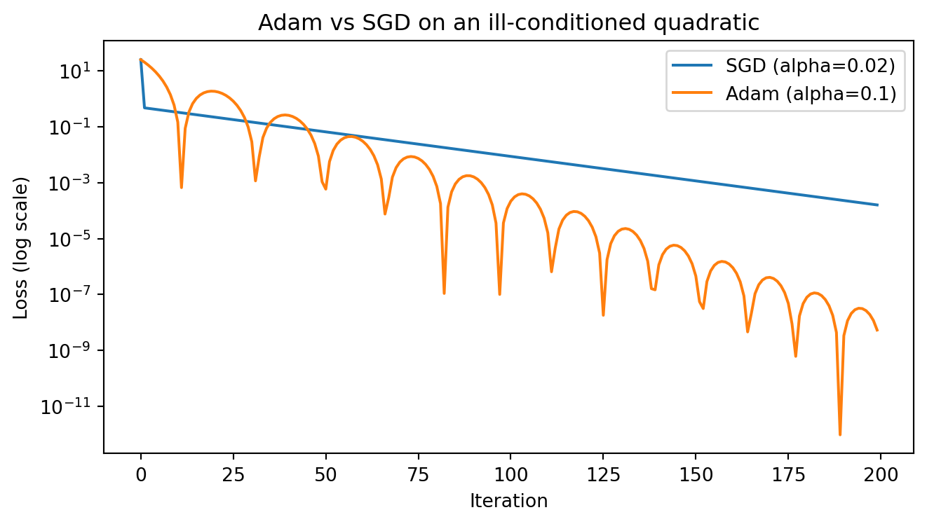
The algorithm in full is a from-scratch numpy optimizer of only a few lines. The cell below implements both Adam and plain SGD, then runs them on an ill-conditioned quadratic, the long narrow ravine described earlier, where the curvature along one axis is fifty times that along the other. Adam’s per-coordinate scaling lets it descend the floor of the ravine far faster than SGD, which must use a small global step to avoid oscillating across the steep walls.
Code
import numpy as npimport matplotlib.pyplot as pltnp.random.seed(0)def loss_and_grad(theta):# Ill-conditioned ravine: f = 0.5*(a*x^2 + b*y^2), curvature ratio 50:1 a, b =1.0, 50.0 x, y = theta f =0.5* (a * x**2+ b * y**2) g = np.array([a * x, b * y])return f, gdef run_sgd(theta0, alpha, steps): theta = theta0.copy() hist = []for _ inrange(steps): f, g = loss_and_grad(theta) hist.append(f) theta = theta - alpha * greturn np.array(hist)def run_adam(theta0, alpha, steps, beta1=0.9, beta2=0.999, eps=1e-8): theta = theta0.copy() m = np.zeros_like(theta) v = np.zeros_like(theta) hist = []for t inrange(1, steps +1): f, g = loss_and_grad(theta) hist.append(f) m = beta1 * m + (1- beta1) * g v = beta2 * v + (1- beta2) * g * g m_hat = m / (1- beta1**t) v_hat = v / (1- beta2**t) theta = theta - alpha * m_hat / (np.sqrt(v_hat) + eps)return np.array(hist)theta0 = np.array([1.0, 1.0])steps =200sgd_hist = run_sgd(theta0, alpha=0.02, steps=steps)adam_hist = run_adam(theta0, alpha=0.1, steps=steps)print(f"SGD final loss: {sgd_hist[-1]:.3e}")print(f"Adam final loss: {adam_hist[-1]:.3e}")plt.figure(figsize=(7, 4))plt.semilogy(sgd_hist, label="SGD (alpha=0.02)")plt.semilogy(adam_hist, label="Adam (alpha=0.1)")plt.xlabel("Iteration")plt.ylabel("Loss (log scale)")plt.title("Adam vs SGD on an ill-conditioned quadratic")plt.legend()plt.tight_layout()plt.show()
SGD  final loss: 1.610e-04
Adam final loss: 5.349e-09
Several features of this rule deserve comment. The numerator \(\hat{m}_t\) is the momentum smoothed gradient, supplying direction and acceleration. The denominator \(\sqrt{\hat{v}_t}\) is the RMSProp normalizer, supplying per-coordinate adaptive scaling. The constant \(\epsilon\), a small positive number, prevents division by zero and bounds the maximum effective step when a coordinate has seen only near-zero gradients.
A revealing way to read the rule is through the ratio \(\hat{m}_t / \sqrt{\hat{v}_t}\), sometimes called the signal to noise ratio of the gradient estimate. When recent gradients agree in sign and magnitude, \(\hat{m}_t\) is large relative to \(\sqrt{\hat{v}_t}\) and the step is close to \(\pm \alpha\) per coordinate. When gradients are noisy and inconsistent, the squared magnitude in \(\hat{v}_t\) stays large while the signed average \(\hat{m}_t\) shrinks through cancellation, so the ratio drops and Adam takes smaller, more cautious steps. This automatic annealing near regions of high gradient noise, often the neighborhood of a minimum, is one reason Adam is robust without manual tuning.
A further consequence is that the update is approximately invariant to the scale of the gradient. If the loss is rescaled by a constant \(c\), then both \(\hat{m}_t\) and \(\sqrt{\hat{v}_t}\) scale by \(c\) and the ratio is unchanged up to the \(\epsilon\) term. This scale invariance is why a single learning rate transfers reasonably well across architectures and loss scalings, in sharp contrast to plain SGD.
201.4.1 4.1 A Convenient Reformulation
Implementations often fold the bias correction into an effective step size to avoid computing \(\hat{m}_t\) and \(\hat{v}_t\) separately. Define
which is algebraically equivalent for an appropriately adjusted \(\hat{\epsilon}\). This form makes clear that bias correction acts as a time varying multiplier on the learning rate, large warmup style scaling at the start that relaxes to the constant \(\alpha\) once the moment estimates have stabilized.
201.5 5. Practical Defaults and Usage
The original paper proposed a set of default hyperparameters that have proven remarkably durable across tasks and remain the recommended starting point.
Hyperparameter
Symbol
Default
Learning rate
\(\alpha\)
\(0.001\)
First moment decay
\(\beta_1\)
\(0.9\)
Second moment decay
\(\beta_2\)
\(0.999\)
Numerical constant
\(\epsilon\)
\(10^{-8}\)
A few notes guide their use in practice.
The learning rate \(\alpha\) is the hyperparameter most worth tuning. Although \(0.001\) is a sound default, large language model training commonly uses values in the range \(10^{-4}\) to \(3 \times 10^{-4}\), and a learning rate schedule, typically linear warmup followed by cosine or inverse square root decay, usually outperforms a constant rate. Warmup is especially helpful with Adam because the second moment estimate is unreliable in the first steps even after bias correction, since it rests on very few samples.
The decay \(\beta_1 = 0.9\) gives the first moment an effective memory of roughly \(1/(1-\beta_1) = 10\) recent gradients, while \(\beta_2 = 0.999\) gives the second moment a memory of about \(1000\), a deliberately longer window so that the per-coordinate scale changes slowly and smoothly. Some large scale transformer recipes lower \(\beta_2\) to \(0.95\) to make the variance estimate more responsive and to improve stability with large batches.
The constant \(\epsilon\) guards against division by zero and caps the largest effective step. The default \(10^{-8}\) suits most cases, but very small values can cause instability when \(\hat{v}_t\) is tiny, and some practitioners raise it to \(10^{-6}\) or higher, particularly in mixed precision training where small denominators interact badly with limited numerical range.
201.5.1 5.1 Weight Decay and AdamW
A common pitfall concerns L2 regularization. Adding a penalty \(\tfrac{\lambda}{2}\lVert\theta\rVert^2\) to the loss injects a term \(\lambda\theta\) into the gradient, which then flows through both moment estimates and gets rescaled by \(\sqrt{\hat{v}_t}\). The result is that the effective regularization strength varies per coordinate and couples to the gradient history, which is rarely the intended behavior. AdamW, due to Loshchilov and Hutter, decouples weight decay from the adaptive update by applying it directly to the parameters,
This decoupled form regularizes every parameter uniformly and generalizes better in practice. For most modern deep learning, AdamW rather than the original Adam is the optimizer of choice, and the decoupled decay is enabled by default in many frameworks.
201.5.2 5.2 When Adam Helps and When It Does Not
Adam excels on problems with sparse or noisy gradients, ill conditioned loss surfaces, and architectures where careful per parameter learning rate tuning would otherwise be required, which describes most large neural networks. Its adaptivity gets training off the ground quickly with little tuning. There is a well documented countervailing observation that on some vision benchmarks well tuned SGD with momentum reaches better final test accuracy than Adam, an apparent generalization gap that motivated AdamW and a line of analysis on the implicit regularization of adaptive methods. The practical takeaway is to treat AdamW as a strong, low friction default, to tune the learning rate and its schedule before anything else, and to remember that the bias correction and decoupled weight decay are not optional refinements but parts of what makes the method behave as intended.
201.6 6. References
Kingma, D. P. and Ba, J. Adam: A Method for Stochastic Optimization. International Conference on Learning Representations, 2015. https://arxiv.org/abs/1412.6980
Tieleman, T. and Hinton, G. Lecture 6.5: RMSProp. Coursera, Neural Networks for Machine Learning, 2012. https://www.cs.toronto.edu/~tijmen/csc321/slides/lecture_slides_lec6.pdf
Loshchilov, I. and Hutter, F. Decoupled Weight Decay Regularization. International Conference on Learning Representations, 2019. https://arxiv.org/abs/1711.05101
Reddi, S. J., Kale, S., and Kumar, S. On the Convergence of Adam and Beyond. International Conference on Learning Representations, 2018. https://arxiv.org/abs/1904.09237
Goodfellow, I., Bengio, Y., and Courville, A. Deep Learning, Chapter 8: Optimization for Training Deep Models. MIT Press, 2016. https://www.deeplearningbook.org/contents/optimization.html
Ruder, S. An Overview of Gradient Descent Optimization Algorithms. 2016. https://arxiv.org/abs/1609.04747
Source Code
# Adaptive Learning Rates: The Adam OptimizerStochastic gradient descent reduces a loss function by stepping in the direction of the negative gradient, but a single global learning rate rarely suits every parameter at once. In deep networks the curvature of the loss surface varies wildly across coordinates, gradients arrive with very different magnitudes, and the scale of those magnitudes drifts as training proceeds. Adam, short for adaptive moment estimation, addresses these difficulties by maintaining running estimates of the gradient and its squared magnitude, then using those estimates to scale each parameter update individually. Introduced by Kingma and Ba in 2015, Adam has become the default optimizer for a large fraction of deep learning practice, from transformers to generative models. This chapter develops Adam from its two parent algorithms, derives its moment estimates and the bias correction that makes them trustworthy early in training, states the full update rule, and closes with the practical defaults that have proven durable.## 1. Background: Two Ideas Adam InheritsAdam is best understood as the fusion of two earlier refinements of plain stochastic gradient descent. Each solves a distinct problem, and Adam keeps both solutions.### 1.1 MomentumPlain SGD updates parameters $\theta$ by$$\theta_t = \theta_{t-1} - \alpha \, g_t,$$where $g_t = \nabla_\theta f_t(\theta_{t-1})$ is the stochastic gradient of the minibatch loss at step $t$ and $\alpha$ is the learning rate. When the loss surface forms a long narrow ravine, this update oscillates across the steep walls while crawling slowly along the gentle floor. Momentum damps the oscillation by accumulating an exponentially weighted average of past gradients,$$v_t = \beta v_{t-1} + (1 - \beta) g_t, \qquad \theta_t = \theta_{t-1} - \alpha \, v_t,$$with $\beta$ typically near $0.9$. The averaged direction $v_t$ reinforces components that point consistently the same way and cancels components that flip sign, so the trajectory accelerates along the ravine floor. This is the first moment idea: track the mean of the gradient.### 1.2 RMSPropA separate problem is that a fixed $\alpha$ is too large for parameters with big gradients and too small for parameters with tiny gradients. RMSProp, proposed by Tieleman and Hinton, adapts the step size per coordinate by dividing the gradient by the square root of a running average of squared gradients,$$s_t = \beta s_{t-1} + (1 - \beta) g_t^2, \qquad \theta_t = \theta_{t-1} - \frac{\alpha}{\sqrt{s_t} + \epsilon}\, g_t,$$where $g_t^2$ denotes the elementwise square. Coordinates whose gradients have been large get a small effective learning rate, and coordinates whose gradients have been small get a large one. This normalization keeps the update roughly the same scale across parameters regardless of raw gradient magnitude. This is the second moment idea: track the mean of the squared gradient.Adam combines momentum, which smooths the direction, with RMSProp, which rescales the magnitude per coordinate.## 2. The First and Second Moment EstimatesAdam maintains two exponential moving averages, one for the gradient and one for its elementwise square. At step $t$, given the gradient $g_t$, the updates are$$m_t = \beta_1 m_{t-1} + (1 - \beta_1)\, g_t,$$$$v_t = \beta_2 v_{t-1} + (1 - \beta_2)\, g_t^2,$$initialized at $m_0 = 0$ and $v_0 = 0$. The vector $m_t$ estimates the first moment of the gradient, its mean, and $v_t$ estimates the second raw moment, the mean of the squared gradient. The decay rates $\beta_1, \beta_2 \in [0, 1)$ control how much history each average retains. A larger $\beta$ gives a longer memory and a smoother estimate; a smaller $\beta$ tracks recent gradients more responsively.It is useful to see why $m_t$ and $v_t$ deserve the name moment estimates. Unrolling the recursion for the first moment gives a weighted sum of all past gradients,$$m_t = (1 - \beta_1) \sum_{i=1}^{t} \beta_1^{\,t-i}\, g_i .$$The weights $(1 - \beta_1)\beta_1^{\,t-i}$ are nonnegative and, in the limit of many steps, sum to one. So $m_t$ is a properly normalized weighted average of the gradient history, with the most recent gradients weighted most heavily and older gradients decaying geometrically. The identical argument applies to $v_t$ with $\beta_2$ and $g_i^2$. Both quantities are therefore exponentially weighted estimates of the corresponding moments of the gradient distribution under the minibatch sampling.## 3. Why Bias Correction Is NeededThe moving averages are initialized to zero, and that initialization introduces a systematic bias toward zero in the early steps. Consider the first moment at step one:$$m_1 = \beta_1 \cdot 0 + (1 - \beta_1) g_1 = (1 - \beta_1) g_1 .$$If $\beta_1 = 0.9$, then $m_1 = 0.1\, g_1$, only a tenth of the gradient. The estimate is badly shrunk toward zero precisely because there is no accumulated history to fill the average. The same shrinkage afflicts $v_t$ even more severely, since $\beta_2$ is usually closer to one.We can quantify the bias exactly. Suppose the gradients $g_i$ are drawn so that the second moment is approximately stationary, $\mathbb{E}[g_i^2] = \mathbb{E}[g_t^2]$ over the relevant window. Taking the expectation of the unrolled second moment estimate,$$\mathbb{E}[v_t] = (1 - \beta_2) \sum_{i=1}^{t} \beta_2^{\,t-i}\, \mathbb{E}[g_i^2]= \mathbb{E}[g_t^2] \, (1 - \beta_2) \sum_{i=1}^{t} \beta_2^{\,t-i} .$$The geometric sum evaluates to $(1 - \beta_2^t)/(1 - \beta_2)$, so$$\mathbb{E}[v_t] = \mathbb{E}[g_t^2] \,\bigl(1 - \beta_2^{\,t}\bigr).$$The factor $1 - \beta_2^{\,t}$ is the source of the bias. Early in training it is much less than one, so $v_t$ underestimates the true second moment. As $t$ grows, $\beta_2^{\,t} \to 0$ and the factor approaches one, so the bias vanishes asymptotically. The analogous result holds for the first moment, $\mathbb{E}[m_t] = \mathbb{E}[g_t]\,(1 - \beta_1^{\,t})$.The remedy follows immediately. Dividing each estimate by its bias factor produces a corrected estimate whose expectation matches the true moment:$$\hat{m}_t = \frac{m_t}{1 - \beta_1^{\,t}}, \qquad \hat{v}_t = \frac{v_t}{1 - \beta_2^{\,t}} .$$These corrected quantities $\hat{m}_t$ and $\hat{v}_t$ are what Adam actually uses in its step. The correction matters most in the opening hundreds or thousands of iterations; once $\beta_1^{\,t}$ and $\beta_2^{\,t}$ have decayed to negligible values, the corrected and uncorrected estimates coincide. Without it, the first updates would be artificially tiny and the per-coordinate scaling would be distorted, which can slow or destabilize the start of training.The plot below traces the two bias-correction denominators across the first thousand steps. The first moment, with $\beta_1 = 0.9$, recovers in a few dozen steps, while the second moment, with $\beta_2 = 0.999$, takes far longer, which is exactly why its early estimate is the more fragile of the two.```{python}import numpy as npimport matplotlib.pyplot as pltnp.random.seed(0)t = np.arange(1, 1001)beta1, beta2 =0.9, 0.999corr1 =1- beta1**tcorr2 =1- beta2**tprint(f"At t=1: 1-b1^t={corr1[0]:.3f}, 1-b2^t={corr2[0]:.4f}")print(f"At t=100: 1-b1^t={corr1[99]:.3f}, 1-b2^t={corr2[99]:.4f}")print(f"At t=1000: 1-b1^t={corr1[-1]:.3f}, 1-b2^t={corr2[-1]:.4f}")plt.figure(figsize=(7, 4))plt.plot(t, corr1, label=r"$1-\beta_1^t$($\beta_1=0.9$)")plt.plot(t, corr2, label=r"$1-\beta_2^t$($\beta_2=0.999$)")plt.axhline(1.0, color="gray", ls="--", lw=0.8)plt.xlabel("Step t")plt.ylabel("Bias-correction denominator")plt.title("How fast the initialization bias decays")plt.legend()plt.tight_layout()plt.show()```## 4. The Adam Update RuleAssembling the pieces gives the complete algorithm. At each step Adam computes the gradient, updates both moving averages, applies bias correction, and takes a scaled step.The algorithm in full is a from-scratch numpy optimizer of only a few lines. The cell below implements both Adam and plain SGD, then runs them on an ill-conditioned quadratic, the long narrow ravine described earlier, where the curvature along one axis is fifty times that along the other. Adam's per-coordinate scaling lets it descend the floor of the ravine far faster than SGD, which must use a small global step to avoid oscillating across the steep walls.```{python}import numpy as npimport matplotlib.pyplot as pltnp.random.seed(0)def loss_and_grad(theta):# Ill-conditioned ravine: f = 0.5*(a*x^2 + b*y^2), curvature ratio 50:1 a, b =1.0, 50.0 x, y = theta f =0.5* (a * x**2+ b * y**2) g = np.array([a * x, b * y])return f, gdef run_sgd(theta0, alpha, steps): theta = theta0.copy() hist = []for _ inrange(steps): f, g = loss_and_grad(theta) hist.append(f) theta = theta - alpha * greturn np.array(hist)def run_adam(theta0, alpha, steps, beta1=0.9, beta2=0.999, eps=1e-8): theta = theta0.copy() m = np.zeros_like(theta) v = np.zeros_like(theta) hist = []for t inrange(1, steps +1): f, g = loss_and_grad(theta) hist.append(f) m = beta1 * m + (1- beta1) * g v = beta2 * v + (1- beta2) * g * g m_hat = m / (1- beta1**t) v_hat = v / (1- beta2**t) theta = theta - alpha * m_hat / (np.sqrt(v_hat) + eps)return np.array(hist)theta0 = np.array([1.0, 1.0])steps =200sgd_hist = run_sgd(theta0, alpha=0.02, steps=steps)adam_hist = run_adam(theta0, alpha=0.1, steps=steps)print(f"SGD final loss: {sgd_hist[-1]:.3e}")print(f"Adam final loss: {adam_hist[-1]:.3e}")plt.figure(figsize=(7, 4))plt.semilogy(sgd_hist, label="SGD (alpha=0.02)")plt.semilogy(adam_hist, label="Adam (alpha=0.1)")plt.xlabel("Iteration")plt.ylabel("Loss (log scale)")plt.title("Adam vs SGD on an ill-conditioned quadratic")plt.legend()plt.tight_layout()plt.show()```The parameter update in closed form is$$\theta_t = \theta_{t-1} - \alpha \, \frac{\hat{m}_t}{\sqrt{\hat{v}_t} + \epsilon} .$$Several features of this rule deserve comment. The numerator $\hat{m}_t$ is the momentum smoothed gradient, supplying direction and acceleration. The denominator $\sqrt{\hat{v}_t}$ is the RMSProp normalizer, supplying per-coordinate adaptive scaling. The constant $\epsilon$, a small positive number, prevents division by zero and bounds the maximum effective step when a coordinate has seen only near-zero gradients.A revealing way to read the rule is through the ratio $\hat{m}_t / \sqrt{\hat{v}_t}$, sometimes called the signal to noise ratio of the gradient estimate. When recent gradients agree in sign and magnitude, $\hat{m}_t$ is large relative to $\sqrt{\hat{v}_t}$ and the step is close to $\pm \alpha$ per coordinate. When gradients are noisy and inconsistent, the squared magnitude in $\hat{v}_t$ stays large while the signed average $\hat{m}_t$ shrinks through cancellation, so the ratio drops and Adam takes smaller, more cautious steps. This automatic annealing near regions of high gradient noise, often the neighborhood of a minimum, is one reason Adam is robust without manual tuning.A further consequence is that the update is approximately invariant to the scale of the gradient. If the loss is rescaled by a constant $c$, then both $\hat{m}_t$ and $\sqrt{\hat{v}_t}$ scale by $c$ and the ratio is unchanged up to the $\epsilon$ term. This scale invariance is why a single learning rate transfers reasonably well across architectures and loss scalings, in sharp contrast to plain SGD.### 4.1 A Convenient ReformulationImplementations often fold the bias correction into an effective step size to avoid computing $\hat{m}_t$ and $\hat{v}_t$ separately. Define$$\alpha_t = \alpha \, \frac{\sqrt{1 - \beta_2^{\,t}}}{1 - \beta_1^{\,t}} .$$The update can then be written using the uncorrected moments directly,$$\theta_t = \theta_{t-1} - \alpha_t \, \frac{m_t}{\sqrt{v_t} + \hat{\epsilon}},$$which is algebraically equivalent for an appropriately adjusted $\hat{\epsilon}$. This form makes clear that bias correction acts as a time varying multiplier on the learning rate, large warmup style scaling at the start that relaxes to the constant $\alpha$ once the moment estimates have stabilized.## 5. Practical Defaults and UsageThe original paper proposed a set of default hyperparameters that have proven remarkably durable across tasks and remain the recommended starting point.| Hyperparameter | Symbol | Default || ---| ---| ---|| Learning rate | $\alpha$ | $0.001$ || First moment decay | $\beta_1$ | $0.9$ || Second moment decay | $\beta_2$ | $0.999$ || Numerical constant | $\epsilon$ | $10^{-8}$ |A few notes guide their use in practice.The learning rate $\alpha$ is the hyperparameter most worth tuning. Although $0.001$ is a sound default, large language model training commonly uses values in the range $10^{-4}$ to $3 \times 10^{-4}$, and a learning rate schedule, typically linear warmup followed by cosine or inverse square root decay, usually outperforms a constant rate. Warmup is especially helpful with Adam because the second moment estimate is unreliable in the first steps even after bias correction, since it rests on very few samples.The decay $\beta_1 = 0.9$ gives the first moment an effective memory of roughly $1/(1-\beta_1) = 10$ recent gradients, while $\beta_2 = 0.999$ gives the second moment a memory of about $1000$, a deliberately longer window so that the per-coordinate scale changes slowly and smoothly. Some large scale transformer recipes lower $\beta_2$ to $0.95$ to make the variance estimate more responsive and to improve stability with large batches.The constant $\epsilon$ guards against division by zero and caps the largest effective step. The default $10^{-8}$ suits most cases, but very small values can cause instability when $\hat{v}_t$ is tiny, and some practitioners raise it to $10^{-6}$ or higher, particularly in mixed precision training where small denominators interact badly with limited numerical range.### 5.1 Weight Decay and AdamWA common pitfall concerns L2 regularization. Adding a penalty $\tfrac{\lambda}{2}\lVert\theta\rVert^2$ to the loss injects a term $\lambda\theta$ into the gradient, which then flows through both moment estimates and gets rescaled by $\sqrt{\hat{v}_t}$. The result is that the effective regularization strength varies per coordinate and couples to the gradient history, which is rarely the intended behavior. AdamW, due to Loshchilov and Hutter, decouples weight decay from the adaptive update by applying it directly to the parameters,$$\theta_t = \theta_{t-1} - \alpha \left( \frac{\hat{m}_t}{\sqrt{\hat{v}_t} + \epsilon} + \lambda\,\theta_{t-1} \right).$$This decoupled form regularizes every parameter uniformly and generalizes better in practice. For most modern deep learning, AdamW rather than the original Adam is the optimizer of choice, and the decoupled decay is enabled by default in many frameworks.### 5.2 When Adam Helps and When It Does NotAdam excels on problems with sparse or noisy gradients, ill conditioned loss surfaces, and architectures where careful per parameter learning rate tuning would otherwise be required, which describes most large neural networks. Its adaptivity gets training off the ground quickly with little tuning. There is a well documented countervailing observation that on some vision benchmarks well tuned SGD with momentum reaches better final test accuracy than Adam, an apparent generalization gap that motivated AdamW and a line of analysis on the implicit regularization of adaptive methods. The practical takeaway is to treat AdamW as a strong, low friction default, to tune the learning rate and its schedule before anything else, and to remember that the bias correction and decoupled weight decay are not optional refinements but parts of what makes the method behave as intended.## 6. References1. Kingma, D. P. and Ba, J. Adam: A Method for Stochastic Optimization. International Conference on Learning Representations, 2015. https://arxiv.org/abs/1412.69802. Tieleman, T. and Hinton, G. Lecture 6.5: RMSProp. Coursera, Neural Networks for Machine Learning, 2012. https://www.cs.toronto.edu/~tijmen/csc321/slides/lecture_slides_lec6.pdf3. Loshchilov, I. and Hutter, F. Decoupled Weight Decay Regularization. International Conference on Learning Representations, 2019. https://arxiv.org/abs/1711.051014. Reddi, S. J., Kale, S., and Kumar, S. On the Convergence of Adam and Beyond. International Conference on Learning Representations, 2018. https://arxiv.org/abs/1904.092375. Goodfellow, I., Bengio, Y., and Courville, A. Deep Learning, Chapter 8: Optimization for Training Deep Models. MIT Press, 2016. https://www.deeplearningbook.org/contents/optimization.html6. Ruder, S. An Overview of Gradient Descent Optimization Algorithms. 2016. https://arxiv.org/abs/1609.04747