The single linear classifier carved a decision surface out of input space with one hyperplane. It is a sharp instrument, but a blunt thinker. Many problems of interest are not solvable by any single hyperplane, and the most famous of these is also one of the simplest: the exclusive-or. The multilayer perceptron (MLP) is the architectural response. By stacking affine transformations and interleaving them with nonlinearities, the MLP learns its own internal coordinate system, a sequence of hidden representations in which a problem that was tangled becomes linearly separable. This chapter develops the MLP from first principles: why stacking matters, how hidden layers reshape geometry, how the forward pass is function composition, and what theory and practice say about trading depth against width.
183.1 1. From One Layer to Many
183.1.1 1.1 The Limits of a Single Affine Map
A single-layer perceptron computes a function of the form
where \(\mathbf{x} \in \mathbb{R}^d\), \(\mathbf{w} \in \mathbb{R}^d\), \(b \in \mathbb{R}\), and \(\sigma\) is a threshold or sigmoid. The decision boundary \(\{\mathbf{x} : \mathbf{w}^\top \mathbf{x} + b = 0\}\) is a hyperplane. The set of functions expressible this way is exactly the set of linearly separable classifications. This is a severe restriction, and it is the restriction that stalled neural network research for over a decade after Minsky and Papert formalized it in 1969 [1].
A natural idea is to chain two affine maps. Let \(\mathbf{h} = W_1 \mathbf{x} + \mathbf{b}_1\) and \(\mathbf{y} = W_2 \mathbf{h} + \mathbf{b}_2\). Composing,
The composition collapses to a single affine map with weight \(W_2 W_1\) and bias \(W_2 \mathbf{b}_1 + \mathbf{b}_2\). No matter how many affine layers we stack, the result is affine. Depth without nonlinearity buys nothing. The nonlinearity is not a cosmetic detail; it is the load-bearing component that makes stacking meaningful.
183.1.2 1.2 The Hidden Layer
The multilayer perceptron repairs this by applying an elementwise nonlinear activation \(\phi\) after each affine map. A one-hidden-layer network is
Here \(W_1 \in \mathbb{R}^{m \times d}\) maps the \(d\) input features to \(m\) hidden units, \(\phi\) acts coordinatewise, and \(W_2 \in \mathbb{R}^{k \times m}\) maps the hidden activations to \(k\) outputs. The vector \(\mathbf{h}\) is the hidden representation. It is neither input nor output. It is a learned intermediate code in which the network reexpresses the data.
The activation \(\phi\) can be the logistic sigmoid \(\phi(z) = 1/(1 + e^{-z})\), the hyperbolic tangent, or, most commonly in modern practice, the rectified linear unit \(\phi(z) = \max(0, z)\) [2]. What every useful choice shares is nonlinearity. Once \(\phi\) is nonlinear, the composition no longer collapses, and the family of representable functions grows dramatically.
183.2 2. Solving XOR
183.2.1 2.1 Why XOR Resists a Line
The exclusive-or function on two binary inputs is defined by
Plot the four points in the unit square. The two positive points \((0,1)\) and \((1,0)\) sit on one diagonal; the two negative points \((0,0)\) and \((1,1)\) sit on the other. No straight line can place both positives on one side and both negatives on the other. Formally, suppose a line \(w_1 x_1 + w_2 x_2 + b = 0\) separated them. The positive cases require \(w_1 + b > 0\) and \(w_2 + b > 0\), while the negative cases require \(b < 0\) and \(w_1 + w_2 + b < 0\). Adding the two positive inequalities gives \(w_1 + w_2 + 2b > 0\), hence \(w_1 + w_2 + b > -b > 0\), contradicting \(w_1 + w_2 + b < 0\). XOR is not linearly separable.
183.2.2 2.2 A Two-Unit Hidden Layer That Works
A single hidden layer with two ReLU units solves it. Consider
with \(\phi(z) = \max(0, z)\). Trace the four inputs. Let \(s = x_1 + x_2\). The first hidden unit computes \(\max(0, s)\) and the second \(\max(0, s - 1)\).
\(\mathbf{x}\)
\(s\)
\(h_1 = \max(0,s)\)
\(h_2 = \max(0,s-1)\)
\(y = h_1 - 2 h_2\)
\((0,0)\)
0
0
0
0
\((0,1)\)
1
1
0
1
\((1,0)\)
1
1
0
1
\((1,1)\)
2
2
1
0
The output reproduces XOR exactly. The mechanism is worth dwelling on. The hidden layer maps the four input points into a new two-dimensional space \((h_1, h_2)\). In that space the positive cases land at \((1,0)\) and the negatives at \((0,0)\) and \((2,1)\). The point \((2,1)\) has been pulled down and to the right, off the diagonal, and now a single output hyperplane \(h_1 - 2 h_2 = 0.5\) cleanly separates the classes. The hidden layer did not classify. It bent the space so that the final linear classifier could.
183.2.3 2.3 The General Lesson
This is the central intuition behind all deep networks. Each hidden layer is a learned change of coordinates. Problems that are entangled in the raw input geometry can become separable, or otherwise tractable, after one or more nonlinear remappings. The network is not memorizing the four XOR points; it is discovering a representation. Scale this idea from four points in two dimensions to millions of images in tens of thousands of dimensions and the same principle drives modern perception systems.
183.3 3. The Forward Pass as Function Composition
183.3.1 3.1 Layers as Functions
An \(L\)-layer MLP is a composition of \(L\) simple functions. Write layer \(\ell\) as
The forward pass is the literal evaluation of this composition. Denoting activations \(\mathbf{a}^{(0)} = \mathbf{x}\) and \(\mathbf{a}^{(\ell)} = f_\ell(\mathbf{a}^{(\ell-1)})\), we compute
and read \(F(\mathbf{x}) = \mathbf{a}^{(L)}\). It is convenient to separate the pre-activation \(\mathbf{z}^{(\ell)} = W_\ell \mathbf{a}^{(\ell-1)} + \mathbf{b}_\ell\) from the post-activation \(\mathbf{a}^{(\ell)} = \phi_\ell(\mathbf{z}^{(\ell)})\), a split that becomes essential when deriving gradients by the chain rule.
The forward pass is a single loop. The cell below builds the hand-derived XOR network from Section 2.2 explicitly and runs it on all four inputs, confirming it reproduces the exclusive-or.
Viewing the network as \(f_L \circ \cdots \circ f_1\) is not merely tidy notation. It clarifies three things at once.
First, it explains training. Because the network is a composition of differentiable functions, its Jacobian factors as a product of per-layer Jacobians by the chain rule. Backpropagation is exactly the reverse-mode accumulation of this product, which is why the pre-activation and post-activation split matters.
Second, it explains representation. The intermediate activations \(\mathbf{a}^{(1)}, \dots, \mathbf{a}^{(L-1)}\) are a hierarchy of representations, each derived from the previous. Empirically, early layers in deep vision networks learn edges and simple textures, while later layers compose these into object parts and whole objects [3]. Composition in the mathematics mirrors composition in the features.
Third, it explains modularity. Layers are interchangeable building blocks. A convolutional layer, an attention block, and a fully connected layer are all just choices of \(f_\ell\). The compositional view is the conceptual interface that lets architectures be assembled from heterogeneous parts.
183.3.3 3.3 Universal Approximation
How expressive is even a single hidden layer? The universal approximation theorem answers this. In the version due to Cybenko [4] and Hornik [5], a feedforward network with one hidden layer and a suitable nonlinear activation can approximate any continuous function on a compact subset of \(\mathbb{R}^d\) to arbitrary accuracy, given enough hidden units. Formally, for any continuous \(g\) on a compact set \(K\) and any \(\varepsilon > 0\), there exist \(m\), weights, and biases such that
This is a reassuring existence result, but it is silent on two practical questions. It does not say how many hidden units \(m\) are required, and that number can be astronomically large. It does not say whether gradient descent can find the needed weights. Universality guarantees that a wide enough shallow network can represent the target. It says nothing about whether that representation is economical or learnable. This gap is precisely what motivates depth.
183.4 4. Depth Versus Width
183.4.1 4.1 Two Ways to Grow a Network
Given a fixed budget of parameters or units, one can spend it on width, many units in few layers, or on depth, fewer units in many layers. Universal approximation says width alone suffices in principle. The theory and practice of the last decade say depth is usually the better investment. The reason is that depth provides exponential expressive efficiency for many natural function classes.
183.4.2 4.2 The Expressive Power of Depth
Consider a deep ReLU network. Each ReLU unit partitions its input space with a hyperplane; a layer of such units carves the space into convex regions, on each of which the network is affine. The number of these linear regions is a useful proxy for the complexity of functions a network can represent. A key result is that the number of linear regions a deep ReLU network can produce grows polynomially in width but exponentially in depth [6]. A network of depth \(L\) and width \(n\) over \(d\) inputs can realize on the order of
\[
\left(\frac{n}{d}\right)^{d(L-1)} n^{d}
\]
linear regions, an expression exponential in \(L\). Intuitively, each layer can fold the input space onto itself, and folds compound multiplicatively through composition. A shallow network must enumerate complex structure piece by piece; a deep network can reuse and recombine intermediate features.
A clean separation theorem makes this concrete. Telgarsky exhibited functions computable by a deep network of \(\Theta(L)\) layers and constant width that require any shallow network to have width exponential in \(L\) to approximate [7]. There exist functions that depth represents compactly and that width can match only at exponential cost. Depth is not just convenient; for some targets it is exponentially more parameter-efficient.
183.4.3 4.3 Why Depth Helps in Practice
The theoretical advantage aligns with an empirical one. Hierarchical, compositional structure is pervasive in real data. Language is characters forming words forming phrases forming meaning; images are pixels forming edges forming parts forming objects. A deep network’s layered representations match this hierarchy, letting each layer build on the abstractions of the previous one rather than reconstructing them from scratch. The breakthrough deep vision models that displaced shallow methods did so largely by going deep, stacking many layers of learned features [3].
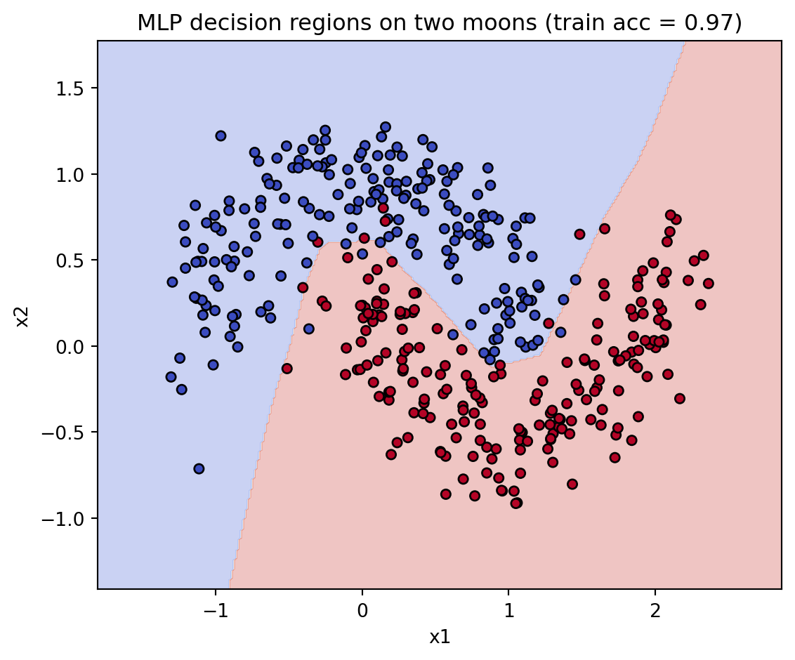
A trained MLP makes the geometry concrete. The cell below fits a small two-hidden-layer network to the two-moons dataset, a problem no single line can separate, and plots the curved decision regions it carves out. The hidden layers bend the space until the two interleaving crescents fall on opposite sides of a learned boundary.
Depth is not free. As networks deepen, gradients propagated back through many layers can shrink toward zero or blow up, the vanishing and exploding gradient problems. Early sigmoid-based deep networks were nearly untrainable for this reason. The practical viability of depth rested on a cluster of innovations: the ReLU activation, which keeps gradients from saturating on the positive side [2]; careful initialization schemes that preserve activation and gradient variance across layers [8]; normalization layers that stabilize the distribution of pre-activations during training; and residual connections that give gradients a direct path backward, enabling networks hundreds of layers deep [9]. Width and depth are therefore not interchangeable knobs. Width tends to be easier to optimize but less efficient, while depth is more expressive but demands architectural care to train.
183.4.5 4.5 A Practical Synthesis
The working guidance that emerges is pragmatic. Enough width is necessary so that no single layer becomes an information bottleneck that discards features the next layer needs. Enough depth is necessary to compose features into the abstractions the task requires. For most modern problems the productive regime is moderately wide and substantially deep, equipped with the stabilizing machinery that makes depth trainable.
The cell below contrasts the two ways of spending a parameter budget on the concentric-circles problem. A single wide hidden layer and a stack of narrow ones both reach the same accuracy here, but the comparison shows that depth and width are distinct allocation choices rather than the same knob.
import numpy as np from sklearn.datasets import make_circles from sklearn.neural_network import MLPClassifier
configs = { “shallow wide (1 x 64)”: (64,), “deep narrow (4 x 10)”: (10, 10, 10, 10), } for name, hidden in configs.items(): m = MLPClassifier(hidden_layer_sizes=hidden, activation=“relu”, max_iter=3000, random_state=rng) m.fit(Xc, yc) n_params = sum(c.size for c in m.coefs_) print(f”{name}: weight params = {n_params}, train acc = {m.score(Xc, yc):.3f}“) ``` The multilayer perceptron, in this light, is the minimal architecture that already exhibits every essential idea of deep learning: stacked affine maps, interleaved nonlinearities, learned hidden representations, the forward pass as composition, and the depth-versus-width tension that governs how that composition is allocated.
183.5 5. Summary
The multilayer perceptron earns its power from a single structural commitment: alternate affine maps with nonlinear activations, and stack the result. Without the nonlinearity, stacking is illusory and the network collapses to one linear map. With it, hidden layers become learned changes of coordinates, as the two-unit solution to XOR shows by bending an inseparable problem into a separable one. The forward pass is the evaluation of a function composition, a frame that simultaneously explains backpropagation, the emergence of hierarchical features, and architectural modularity. Universal approximation guarantees that even a shallow network can represent any continuous target, but depth is what makes the representation efficient and learnable, offering exponential gains in expressivity at the price of optimization difficulties that modern techniques have largely tamed.
183.6 References
M. Minsky and S. Papert, Perceptrons: An Introduction to Computational Geometry, MIT Press, 1969. https://mitpress.mit.edu/9780262630221/perceptrons/
V. Nair and G. E. Hinton, “Rectified Linear Units Improve Restricted Boltzmann Machines,” ICML, 2010. https://www.cs.toronto.edu/~fritz/absps/reluICML.pdf
A. Krizhevsky, I. Sutskever, and G. E. Hinton, “ImageNet Classification with Deep Convolutional Neural Networks,” NeurIPS, 2012. https://papers.nips.cc/paper/4824-imagenet-classification-with-deep-convolutional-neural-networks
G. Cybenko, “Approximation by Superpositions of a Sigmoidal Function,” Mathematics of Control, Signals and Systems, vol. 2, pp. 303 to 314, 1989. https://link.springer.com/article/10.1007/BF02551274
K. Hornik, “Approximation Capabilities of Multilayer Feedforward Networks,” Neural Networks, vol. 4, no. 2, pp. 251 to 257, 1991. https://doi.org/10.1016/0893-6080(91)90009-T
G. Montufar, R. Pascanu, K. Cho, and Y. Bengio, “On the Number of Linear Regions of Deep Neural Networks,” NeurIPS, 2014. https://papers.nips.cc/paper/5422-on-the-number-of-linear-regions-of-deep-neural-networks
M. Telgarsky, “Benefits of Depth in Neural Networks,” COLT, 2016. https://proceedings.mlr.press/v49/telgarsky16.html
X. Glorot and Y. Bengio, “Understanding the Difficulty of Training Deep Feedforward Neural Networks,” AISTATS, 2010. https://proceedings.mlr.press/v9/glorot10a.html
K. He, X. Zhang, S. Ren, and J. Sun, “Deep Residual Learning for Image Recognition,” CVPR, 2016. https://openaccess.thecvf.com/content_cvpr_2016/html/He_Deep_Residual_Learning_CVPR_2016_paper.html
Source Code
# Multilayer PerceptronsThe single linear classifier carved a decision surface out of input space with one hyperplane. It is a sharp instrument, but a blunt thinker. Many problems of interest are not solvable by any single hyperplane, and the most famous of these is also one of the simplest: the exclusive-or. The multilayer perceptron (MLP) is the architectural response. By stacking affine transformations and interleaving them with nonlinearities, the MLP learns its own internal coordinate system, a sequence of hidden representations in which a problem that was tangled becomes linearly separable. This chapter develops the MLP from first principles: why stacking matters, how hidden layers reshape geometry, how the forward pass is function composition, and what theory and practice say about trading depth against width.## 1. From One Layer to Many### 1.1 The Limits of a Single Affine MapA single-layer perceptron computes a function of the form$$f(\mathbf{x}) = \sigma(\mathbf{w}^\top \mathbf{x} + b),$$where $\mathbf{x} \in \mathbb{R}^d$, $\mathbf{w} \in \mathbb{R}^d$, $b \in \mathbb{R}$, and $\sigma$ is a threshold or sigmoid. The decision boundary $\{\mathbf{x} : \mathbf{w}^\top \mathbf{x} + b = 0\}$ is a hyperplane. The set of functions expressible this way is exactly the set of linearly separable classifications. This is a severe restriction, and it is the restriction that stalled neural network research for over a decade after Minsky and Papert formalized it in 1969 [1].A natural idea is to chain two affine maps. Let $\mathbf{h} = W_1 \mathbf{x} + \mathbf{b}_1$ and $\mathbf{y} = W_2 \mathbf{h} + \mathbf{b}_2$. Composing,$$\mathbf{y} = W_2 (W_1 \mathbf{x} + \mathbf{b}_1) + \mathbf{b}_2 = (W_2 W_1)\mathbf{x} + (W_2 \mathbf{b}_1 + \mathbf{b}_2).$$The composition collapses to a single affine map with weight $W_2 W_1$ and bias $W_2 \mathbf{b}_1 + \mathbf{b}_2$. No matter how many affine layers we stack, the result is affine. Depth without nonlinearity buys nothing. The nonlinearity is not a cosmetic detail; it is the load-bearing component that makes stacking meaningful.### 1.2 The Hidden LayerThe multilayer perceptron repairs this by applying an elementwise nonlinear activation $\phi$ after each affine map. A one-hidden-layer network is$$\mathbf{h} = \phi(W_1 \mathbf{x} + \mathbf{b}_1), \qquad\mathbf{y} = W_2 \mathbf{h} + \mathbf{b}_2.$$Here $W_1 \in \mathbb{R}^{m \times d}$ maps the $d$ input features to $m$ hidden units, $\phi$ acts coordinatewise, and $W_2 \in \mathbb{R}^{k \times m}$ maps the hidden activations to $k$ outputs. The vector $\mathbf{h}$ is the hidden representation. It is neither input nor output. It is a learned intermediate code in which the network reexpresses the data.The activation $\phi$ can be the logistic sigmoid $\phi(z) = 1/(1 + e^{-z})$, the hyperbolic tangent, or, most commonly in modern practice, the rectified linear unit $\phi(z) = \max(0, z)$ [2]. What every useful choice shares is nonlinearity. Once $\phi$ is nonlinear, the composition no longer collapses, and the family of representable functions grows dramatically.## 2. Solving XOR### 2.1 Why XOR Resists a LineThe exclusive-or function on two binary inputs is defined by$$\text{XOR}(0,0) = 0, \quad \text{XOR}(0,1) = 1, \quad \text{XOR}(1,0) = 1, \quad \text{XOR}(1,1) = 0.$$Plot the four points in the unit square. The two positive points $(0,1)$ and $(1,0)$ sit on one diagonal; the two negative points $(0,0)$ and $(1,1)$ sit on the other. No straight line can place both positives on one side and both negatives on the other. Formally, suppose a line $w_1 x_1 + w_2 x_2 + b = 0$ separated them. The positive cases require $w_1 + b > 0$ and $w_2 + b > 0$, while the negative cases require $b < 0$ and $w_1 + w_2 + b < 0$. Adding the two positive inequalities gives $w_1 + w_2 + 2b > 0$, hence $w_1 + w_2 + b > -b > 0$, contradicting $w_1 + w_2 + b < 0$. XOR is not linearly separable.### 2.2 A Two-Unit Hidden Layer That WorksA single hidden layer with two ReLU units solves it. Consider$$\mathbf{h} = \phi\!\left(\begin{bmatrix} 1 & 1 \\ 1 & 1 \end{bmatrix} \mathbf{x}+ \begin{bmatrix} 0 \\ -1 \end{bmatrix}\right), \qquady = \begin{bmatrix} 1 & -2 \end{bmatrix} \mathbf{h} + 0,$$with $\phi(z) = \max(0, z)$. Trace the four inputs. Let $s = x_1 + x_2$. The first hidden unit computes $\max(0, s)$ and the second $\max(0, s - 1)$.| $\mathbf{x}$ | $s$ | $h_1 = \max(0,s)$ | $h_2 = \max(0,s-1)$ | $y = h_1 - 2 h_2$ ||---|---|---|---|---|| $(0,0)$ | 0 | 0 | 0 | 0 || $(0,1)$ | 1 | 1 | 0 | 1 || $(1,0)$ | 1 | 1 | 0 | 1 || $(1,1)$ | 2 | 2 | 1 | 0 |The output reproduces XOR exactly. The mechanism is worth dwelling on. The hidden layer maps the four input points into a new two-dimensional space $(h_1, h_2)$. In that space the positive cases land at $(1,0)$ and the negatives at $(0,0)$ and $(2,1)$. The point $(2,1)$ has been pulled down and to the right, off the diagonal, and now a single output hyperplane $h_1 - 2 h_2 = 0.5$ cleanly separates the classes. The hidden layer did not classify. It bent the space so that the final linear classifier could.### 2.3 The General LessonThis is the central intuition behind all deep networks. Each hidden layer is a learned change of coordinates. Problems that are entangled in the raw input geometry can become separable, or otherwise tractable, after one or more nonlinear remappings. The network is not memorizing the four XOR points; it is discovering a representation. Scale this idea from four points in two dimensions to millions of images in tens of thousands of dimensions and the same principle drives modern perception systems.## 3. The Forward Pass as Function Composition### 3.1 Layers as FunctionsAn $L$-layer MLP is a composition of $L$ simple functions. Write layer $\ell$ as$$f_\ell(\mathbf{a}) = \phi_\ell(W_\ell \mathbf{a} + \mathbf{b}_\ell).$$Each $f_\ell$ is an affine map followed by an elementwise nonlinearity. The full network is$$F(\mathbf{x}) = f_L \circ f_{L-1} \circ \cdots \circ f_1 (\mathbf{x}).$$The forward pass is the literal evaluation of this composition. Denoting activations $\mathbf{a}^{(0)} = \mathbf{x}$ and $\mathbf{a}^{(\ell)} = f_\ell(\mathbf{a}^{(\ell-1)})$, we compute$$\mathbf{a}^{(\ell)} = \phi_\ell\!\left(W_\ell \mathbf{a}^{(\ell-1)} + \mathbf{b}_\ell\right), \qquad \ell = 1, \dots, L,$$and read $F(\mathbf{x}) = \mathbf{a}^{(L)}$. It is convenient to separate the pre-activation $\mathbf{z}^{(\ell)} = W_\ell \mathbf{a}^{(\ell-1)} + \mathbf{b}_\ell$ from the post-activation $\mathbf{a}^{(\ell)} = \phi_\ell(\mathbf{z}^{(\ell)})$, a split that becomes essential when deriving gradients by the chain rule.The forward pass is a single loop. The cell below builds the hand-derived XOR network from Section 2.2 explicitly and runs it on all four inputs, confirming it reproduces the exclusive-or.```{python}import numpy as npX = np.array([[0, 0], [0, 1], [1, 0], [1, 1]], dtype=float)W1 = np.array([[1.0, 1.0], [1.0, 1.0]])b1 = np.array([0.0, -1.0])W2 = np.array([1.0, -2.0])b2 =0.0def relu(z):return np.maximum(0.0, z)# forward pass as composition: affine, nonlinearity, affineH = relu(X @ W1.T + b1)y = H @ W2 + b2print("input -> hidden -> output")for xi, hi, yi inzip(X, H, y):print(f"{xi.astype(int)} h={hi} y={yi:.1f}")print("XOR reproduced:", np.allclose(y, [0, 1, 1, 0]))```### 3.2 Why Composition Is the Right FrameViewing the network as $f_L \circ \cdots \circ f_1$ is not merely tidy notation. It clarifies three things at once.First, it explains training. Because the network is a composition of differentiable functions, its Jacobian factors as a product of per-layer Jacobians by the chain rule. Backpropagation is exactly the reverse-mode accumulation of this product, which is why the pre-activation and post-activation split matters.Second, it explains representation. The intermediate activations $\mathbf{a}^{(1)}, \dots, \mathbf{a}^{(L-1)}$ are a hierarchy of representations, each derived from the previous. Empirically, early layers in deep vision networks learn edges and simple textures, while later layers compose these into object parts and whole objects [3]. Composition in the mathematics mirrors composition in the features.Third, it explains modularity. Layers are interchangeable building blocks. A convolutional layer, an attention block, and a fully connected layer are all just choices of $f_\ell$. The compositional view is the conceptual interface that lets architectures be assembled from heterogeneous parts.### 3.3 Universal ApproximationHow expressive is even a single hidden layer? The universal approximation theorem answers this. In the version due to Cybenko [4] and Hornik [5], a feedforward network with one hidden layer and a suitable nonlinear activation can approximate any continuous function on a compact subset of $\mathbb{R}^d$ to arbitrary accuracy, given enough hidden units. Formally, for any continuous $g$ on a compact set $K$ and any $\varepsilon > 0$, there exist $m$, weights, and biases such that$$\sup_{\mathbf{x} \in K} \left| g(\mathbf{x}) - \sum_{i=1}^{m} c_i \, \phi(\mathbf{w}_i^\top \mathbf{x} + b_i) \right| < \varepsilon.$$This is a reassuring existence result, but it is silent on two practical questions. It does not say how many hidden units $m$ are required, and that number can be astronomically large. It does not say whether gradient descent can find the needed weights. Universality guarantees that a wide enough shallow network can represent the target. It says nothing about whether that representation is economical or learnable. This gap is precisely what motivates depth.## 4. Depth Versus Width### 4.1 Two Ways to Grow a NetworkGiven a fixed budget of parameters or units, one can spend it on width, many units in few layers, or on depth, fewer units in many layers. Universal approximation says width alone suffices in principle. The theory and practice of the last decade say depth is usually the better investment. The reason is that depth provides exponential expressive efficiency for many natural function classes.### 4.2 The Expressive Power of DepthConsider a deep ReLU network. Each ReLU unit partitions its input space with a hyperplane; a layer of such units carves the space into convex regions, on each of which the network is affine. The number of these linear regions is a useful proxy for the complexity of functions a network can represent. A key result is that the number of linear regions a deep ReLU network can produce grows polynomially in width but exponentially in depth [6]. A network of depth $L$ and width $n$ over $d$ inputs can realize on the order of$$\left(\frac{n}{d}\right)^{d(L-1)} n^{d}$$linear regions, an expression exponential in $L$. Intuitively, each layer can fold the input space onto itself, and folds compound multiplicatively through composition. A shallow network must enumerate complex structure piece by piece; a deep network can reuse and recombine intermediate features.A clean separation theorem makes this concrete. Telgarsky exhibited functions computable by a deep network of $\Theta(L)$ layers and constant width that require any shallow network to have width exponential in $L$ to approximate [7]. There exist functions that depth represents compactly and that width can match only at exponential cost. Depth is not just convenient; for some targets it is exponentially more parameter-efficient.### 4.3 Why Depth Helps in PracticeThe theoretical advantage aligns with an empirical one. Hierarchical, compositional structure is pervasive in real data. Language is characters forming words forming phrases forming meaning; images are pixels forming edges forming parts forming objects. A deep network's layered representations match this hierarchy, letting each layer build on the abstractions of the previous one rather than reconstructing them from scratch. The breakthrough deep vision models that displaced shallow methods did so largely by going deep, stacking many layers of learned features [3].A trained MLP makes the geometry concrete. The cell below fits a small two-hidden-layer network to the two-moons dataset, a problem no single line can separate, and plots the curved decision regions it carves out. The hidden layers bend the space until the two interleaving crescents fall on opposite sides of a learned boundary.```{python}import numpy as npimport matplotlib.pyplot as pltfrom sklearn.datasets import make_moonsfrom sklearn.neural_network import MLPClassifierrng =42Xm, ym = make_moons(n_samples=400, noise=0.20, random_state=rng)clf = MLPClassifier(hidden_layer_sizes=(16, 16), activation="relu", max_iter=2000, random_state=rng)clf.fit(Xm, ym)acc = clf.score(Xm, ym)x_min, x_max = Xm[:, 0].min() -0.5, Xm[:, 0].max() +0.5y_min, y_max = Xm[:, 1].min() -0.5, Xm[:, 1].max() +0.5xx, yy = np.meshgrid(np.linspace(x_min, x_max, 300), np.linspace(y_min, y_max, 300))Z = clf.predict(np.c_[xx.ravel(), yy.ravel()]).reshape(xx.shape)fig, ax = plt.subplots(figsize=(6, 5))ax.contourf(xx, yy, Z, alpha=0.3, cmap="coolwarm")ax.scatter(Xm[:, 0], Xm[:, 1], c=ym, cmap="coolwarm", edgecolor="k", s=25)ax.set_title(f"MLP decision regions on two moons (train acc = {acc:.2f})")ax.set_xlabel("x1")ax.set_ylabel("x2")plt.tight_layout()plt.show()```### 4.4 The Costs of DepthDepth is not free. As networks deepen, gradients propagated back through many layers can shrink toward zero or blow up, the vanishing and exploding gradient problems. Early sigmoid-based deep networks were nearly untrainable for this reason. The practical viability of depth rested on a cluster of innovations: the ReLU activation, which keeps gradients from saturating on the positive side [2]; careful initialization schemes that preserve activation and gradient variance across layers [8]; normalization layers that stabilize the distribution of pre-activations during training; and residual connections that give gradients a direct path backward, enabling networks hundreds of layers deep [9]. Width and depth are therefore not interchangeable knobs. Width tends to be easier to optimize but less efficient, while depth is more expressive but demands architectural care to train.### 4.5 A Practical SynthesisThe working guidance that emerges is pragmatic. Enough width is necessary so that no single layer becomes an information bottleneck that discards features the next layer needs. Enough depth is necessary to compose features into the abstractions the task requires. For most modern problems the productive regime is moderately wide and substantially deep, equipped with the stabilizing machinery that makes depth trainable.The cell below contrasts the two ways of spending a parameter budget on the concentric-circles problem. A single wide hidden layer and a stack of narrow ones both reach the same accuracy here, but the comparison shows that depth and width are distinct allocation choices rather than the same knob.```{python}import numpy as npfrom sklearn.datasets import make_circlesfrom sklearn.neural_network import MLPClassifierrng =0Xc, yc = make_circles(n_samples=500, noise=0.10, factor=0.4, random_state=rng)configs = {"shallow wide (1 x 64)": (64,),"deep narrow (4 x 10)": (10, 10, 10, 10),}for name, hidden in configs.items(): m = MLPClassifier(hidden_layer_sizes=hidden, activation="relu", max_iter=3000, random_state=rng) m.fit(Xc, yc) n_params =sum(c.size for c in m.coefs_)print(f"{name}: weight params = {n_params}, train acc = {m.score(Xc, yc):.3f}")``` The multilayer perceptron, in this light, is the minimal architecture that already exhibits every essential idea of deep learning: stacked affine maps, interleaved nonlinearities, learned hidden representations, the forward passas composition, and the depth-versus-width tension that governs how that composition is allocated.## 5. SummaryThe multilayer perceptron earns its power from a single structural commitment: alternate affine maps with nonlinear activations, and stack the result. Without the nonlinearity, stacking is illusory and the network collapses to one linear map. With it, hidden layers become learned changes of coordinates, as the two-unit solution to XOR shows by bending an inseparable problem into a separable one. The forward passis the evaluation of a function composition, a frame that simultaneously explains backpropagation, the emergence of hierarchical features, and architectural modularity. Universal approximation guarantees that even a shallow network can represent any continuous target, but depth is what makes the representation efficient and learnable, offering exponential gains in expressivity at the price of optimization difficulties that modern techniques have largely tamed.## References1. M. Minsky and S. Papert, *Perceptrons: An Introduction to Computational Geometry*, MIT Press, 1969. https://mitpress.mit.edu/9780262630221/perceptrons/2. V. Nair and G. E. Hinton, "Rectified Linear Units Improve Restricted Boltzmann Machines," ICML, 2010. https://www.cs.toronto.edu/~fritz/absps/reluICML.pdf3. A. Krizhevsky, I. Sutskever, and G. E. Hinton, "ImageNet Classification with Deep Convolutional Neural Networks," NeurIPS, 2012. https://papers.nips.cc/paper/4824-imagenet-classification-with-deep-convolutional-neural-networks4. G. Cybenko, "Approximation by Superpositions of a Sigmoidal Function,"*Mathematics of Control, Signals and Systems*, vol. 2, pp. 303 to 314, 1989. https://link.springer.com/article/10.1007/BF025512745. K. Hornik, "Approximation Capabilities of Multilayer Feedforward Networks,"*Neural Networks*, vol. 4, no. 2, pp. 251 to 257, 1991. https://doi.org/10.1016/0893-6080(91)90009-T6. G. Montufar, R. Pascanu, K. Cho, and Y. Bengio, "On the Number of Linear Regions of Deep Neural Networks," NeurIPS, 2014. https://papers.nips.cc/paper/5422-on-the-number-of-linear-regions-of-deep-neural-networks7. M. Telgarsky, "Benefits of Depth in Neural Networks," COLT, 2016. https://proceedings.mlr.press/v49/telgarsky16.html8. X. Glorot and Y. Bengio, "Understanding the Difficulty of Training Deep Feedforward Neural Networks," AISTATS, 2010. https://proceedings.mlr.press/v9/glorot10a.html9. K. He, X. Zhang, S. Ren, and J. Sun, "Deep Residual Learning for Image Recognition," CVPR, 2016. https://openaccess.thecvf.com/content_cvpr_2016/html/He_Deep_Residual_Learning_CVPR_2016_paper.html