Ordinary least squares regression rests on a comfortable but restrictive set of assumptions: the response is continuous, its conditional mean is a linear function of the predictors, and the noise around that mean is Gaussian with constant variance. A great deal of real data violates these assumptions in obvious ways. Counts of events are nonnegative integers. Binary outcomes live in \(\{0, 1\}\). Proportions are bounded between zero and one. Waiting times are positive and skewed. Forcing a linear Gaussian model onto such data produces predictions that fall outside the valid range and standard errors that are simply wrong.
Generalized Linear Models, introduced by Nelder and Wedderburn in 1972, provide a single coherent framework that accommodates all of these cases. The key insight is that linear regression, logistic regression, and Poisson regression are not three unrelated techniques but three instances of one model class, differing only in two choices: the probability distribution assumed for the response and the function that connects the linear predictor to the mean. Once you see the unifying structure, a single estimation algorithm fits all of them, a single notion of residual deviance measures fit across all of them, and the asymptotic inference theory transfers wholesale. This chapter develops that structure from the exponential family upward and shows how it pays off in practice.
95.1 1. The Exponential Family
95.1.1 1.1 Canonical form
A distribution belongs to the one parameter exponential family if its density or mass function can be written as
Here \(\theta\) is the natural or canonical parameter, \(\phi\) is a dispersion parameter, and \(a\), \(b\), \(c\) are known functions that specify the particular distribution. The function \(b(\theta)\) is called the cumulant function and it carries all the information we need about the mean and variance.
This form looks abstract, but many familiar distributions fit it after light algebra. Consider the Gaussian with known variance \(\sigma^2\):
Matching terms gives \(\theta = \mu\), \(b(\theta) = \theta^2/2\), \(a(\phi) = \sigma^2\), and \(c(y, \phi)\) collects the remaining pieces. The Bernoulli, binomial, Poisson, gamma, and inverse Gaussian distributions all admit analogous representations.
95.1.2 1.2 Mean and variance from the cumulant function
The cumulant function earns its name because its derivatives generate the moments of \(Y\). The derivation is worth carrying out, because it shows that the mean and variance are not separate assumptions but consequences of the canonical form. Begin from the log likelihood of a single observation,
The first follows from differentiating \(\int f \, dy = 1\) under the integral sign; the second is the differentiated form of the same identity. The derivatives of \(\ell\) are immediate from the canonical form,
Substituting the first derivative into \(\mathbb{E}[\partial \ell / \partial \theta] = 0\) gives \(\mathbb{E}[y - b'(\theta)] = 0\), hence \(\mu = b'(\theta)\). Substituting both derivatives into the second identity gives
The first identity says the mean is the derivative of the cumulant function with respect to the natural parameter. The second says the variance factors into a dispersion piece \(a(\phi)\) and a piece \(b''(\theta)\) that depends only on the mean. Because \(\mu = b'(\theta)\) is a function of \(\theta\) alone, we can express \(b''(\theta)\) as a function of \(\mu\), which defines the variance function
\[
V(\mu) = b''(\theta(\mu)).
\]
The variance function is the signature of a GLM family. For the Gaussian, \(b''(\theta) = 1\), so \(V(\mu) = 1\) and the variance is constant. For the Poisson, \(V(\mu) = \mu\), so variance equals the mean. For the Bernoulli, \(V(\mu) = \mu(1 - \mu)\), which vanishes at the extremes and peaks at \(\mu = 1/2\). These mean variance relationships are precisely the empirical patterns we observe in counts and binary data, and the exponential family encodes them as a mathematical consequence rather than an ad hoc assumption.
Typically \(a(\phi) = \phi / w\) where \(w\) is a known prior weight, such as the number of binomial trials or a case weight. For the Poisson and binomial the dispersion is fixed at \(\phi = 1\); for the Gaussian and gamma it is a free parameter estimated from the data.
95.2 2. The GLM Framework
95.2.1 2.1 Three components
A generalized linear model is fully specified by three components.
First, a random component: the response \(Y_i\) given covariates is drawn independently from an exponential family distribution with mean \(\mu_i\).
Second, a systematic component: a linear predictor \(\eta_i = \mathbf{x}_i^\top \boldsymbol{\beta}\) combines the covariates through a vector of coefficients \(\boldsymbol{\beta}\).
Third, a link function\(g\) that connects the two through \(g(\mu_i) = \eta_i\). The link is a smooth, monotone, invertible function, so we can also write \(\mu_i = g^{-1}(\eta_i)\), where \(g^{-1}\) is sometimes called the mean function or inverse link.
The separation of these three components is what gives the framework its flexibility. The random component fixes the variance function and the likelihood. The systematic component keeps the convenience of linearity in the parameters. The link function bridges them and, crucially, lets us map an unbounded linear predictor onto a constrained mean.
95.2.2 2.2 Why the link matters
Suppose we model counts. The mean \(\mu_i\) must be positive, but the linear predictor \(\mathbf{x}_i^\top \boldsymbol{\beta}\) ranges over the whole real line. A log link \(g(\mu) = \log \mu\) resolves the tension: \(\mu_i = \exp(\mathbf{x}_i^\top \boldsymbol{\beta})\) is automatically positive for any \(\boldsymbol{\beta}\). For binary data the mean is a probability in \((0, 1)\), and the logit link \(g(\mu) = \log\{\mu / (1 - \mu)\}\) maps that interval onto the real line, with the logistic function as its inverse. The link does the work of respecting the natural constraints of the data while preserving a linear structure for the predictors.
95.2.3 2.3 The canonical link
Among all valid links, one is distinguished. The canonical link sets the linear predictor equal to the natural parameter, \(\eta = \theta\). Equivalently, \(g\) is chosen so that \(g(\mu) = \theta(\mu) = (b')^{-1}(\mu)\). The canonical links are:
Family
Variance \(V(\mu)\)
Canonical link \(g(\mu)\)
Mean function
Gaussian
\(1\)
identity, \(\mu\)
\(\eta\)
Binomial
\(\mu(1-\mu)\)
logit, \(\log\frac{\mu}{1-\mu}\)
\(\frac{1}{1+e^{-\eta}}\)
Poisson
\(\mu\)
log, \(\log\mu\)
\(e^{\eta}\)
Gamma
\(\mu^2\)
inverse, \(-1/\mu\)
\(-1/\eta\)
Canonical links carry several conveniences. The sufficient statistic for \(\boldsymbol{\beta}\) becomes \(\mathbf{X}^\top \mathbf{y}\), the observed and expected information matrices coincide, and the score equations take a particularly clean form. You are not obligated to use the canonical link, and sometimes another choice fits the science better. The probit link for binary data and the identity link for Poisson rates both have legitimate uses. But the canonical link is the default for good reasons, and we exploit its properties when deriving the estimator below.
95.3 3. Maximum Likelihood Estimation
95.3.1 3.1 The log likelihood and score
We estimate \(\boldsymbol{\beta}\) by maximum likelihood. For independent observations the log likelihood is the sum of individual contributions,
To differentiate with respect to \(\boldsymbol{\beta}\) we apply the chain rule through the chain \(\boldsymbol{\beta} \to \eta_i \to \mu_i \to \theta_i\). Using \(\partial \theta_i / \partial \mu_i = 1 / V(\mu_i)\), \(\partial \mu_i / \partial \eta_i = 1 / g'(\mu_i)\), and \(\partial \eta_i / \partial \boldsymbol{\beta} = \mathbf{x}_i\), the score function works out to
Setting this to zero gives the estimating equations. Notice the appealing structure: each observation contributes its residual \(y_i - \mu_i\), weighted by a term that depends on the variance and the slope of the link, projected onto the covariate vector. Under the canonical link the messy weighting simplifies, and the score equations reduce to \(\mathbf{X}^\top (\mathbf{y} - \boldsymbol{\mu}) = \mathbf{0}\), which says the model matches the data in the directions spanned by the covariates.
95.3.2 3.2 No closed form in general
Except for the Gaussian identity link case, which recovers ordinary least squares, these equations are nonlinear in \(\boldsymbol{\beta}\) because \(\mu_i\) depends on \(\boldsymbol{\beta}\) through a nonlinear inverse link. There is no closed form solution. We need an iterative numerical method, and the structure of the exponential family hands us a particularly elegant one.
95.4 4. Iteratively Reweighted Least Squares
95.4.1 4.1 Newton Raphson meets Fisher scoring
The natural way to solve the score equations is Newton Raphson, which iterates
where \(\mathbf{u}\) is the score and \(\mathbf{H}\) is the negative Hessian. Fisher scoring replaces the observed Hessian with its expectation, the Fisher information matrix \(\mathcal{I} = \mathbb{E}[-\mathbf{H}]\). For GLMs this expectation has a clean form, and under the canonical link the observed and expected Hessians are identical, so the two methods coincide. The Fisher information for a GLM is
where \(\mathbf{W}\) is a diagonal matrix of weights \(w_i = 1 / \{ a_i(\phi)\, V(\mu_i)\, g'(\mu_i)^2 \}\).
95.4.2 4.2 The working response
The remarkable fact is that each Fisher scoring step can be rewritten as a weighted least squares regression. To see why, write the Fisher scoring update in full,
where the score from Section 3.1 has been factored as \(\mathbf{u} = \mathbf{X}^\top \mathbf{W} \mathbf{r}\) with residual vector entries \(r_i = (y_i - \mu_i)\, g'(\mu_i)\). This factorization follows by writing the score weight \(1 / \{ a_i(\phi)\, V(\mu_i)\, g'(\mu_i) \}\) as \(w_i \cdot g'(\mu_i)\), with \(w_i = 1 / \{ a_i(\phi)\, V(\mu_i)\, g'(\mu_i)^2 \}\) matching the Fisher information weights. Now pull the leading \(\boldsymbol{\beta}^{(t)}\) inside by noting \(\boldsymbol{\beta}^{(t)} = (\mathbf{X}^\top \mathbf{W} \mathbf{X})^{-1} \mathbf{X}^\top \mathbf{W} \mathbf{X} \boldsymbol{\beta}^{(t)}\) and that \(\mathbf{X}\boldsymbol{\beta}^{(t)} = \boldsymbol{\eta}\), which gives
The bracketed quantity is the working response, sometimes called the adjusted dependent variable,
\[
z_i = \eta_i + (y_i - \mu_i)\, g'(\mu_i).
\]
This is a first order Taylor expansion of the link applied to the data: it linearizes \(g(y_i)\) around the current fitted mean. With the weights \(w_i\) above, the Fisher scoring update is therefore exactly the solution of a weighted least squares problem,
Because both the weights \(\mathbf{W}\) and the working response \(\mathbf{z}\) depend on the current estimate of \(\boldsymbol{\beta}\) through \(\mu_i\) and \(\eta_i\), we recompute them at every iteration. Hence the name: Iteratively Reweighted Least Squares, or IRLS.
95.4.3 4.3 The algorithm
The procedure is compact and the same code fits every family.
The iteratively reweighted least squares (IRLS) procedure is:
Initialize \(\mu\) from the data (often \(\mu = y\), lightly adjusted) and set the linear predictor \(\eta = g(\mu)\).
Repeat until convergence:
Working response: \(z = \eta + (y - \mu)\,g'(\mu)\)
Working weights: \(w = \dfrac{1}{a(\phi)\,V(\mu)\,g'(\mu)^2}\)
Weighted least squares: \(\beta = (X^\top W X)^{-1} X^\top W z\), with \(W = \operatorname{diag}(w)\)
Update: \(\eta = X\beta\), then \(\mu = g^{-1}(\eta)\)
Each iteration is a single weighted regression, which off the shelf linear algebra handles efficiently and stably, for instance through a QR or Cholesky decomposition rather than explicit matrix inversion. Because the GLM log likelihood with a canonical link is concave in \(\boldsymbol{\beta}\), IRLS converges to the global maximum from essentially any starting point, usually in a handful of iterations. This is the practical payoff of the exponential family structure: one algorithm, provably well behaved, for the entire model class.
95.4.4 4.4 Standard errors for free
Convergence yields more than point estimates. The inverse of the Fisher information at the solution, \((\mathbf{X}^\top \mathbf{W} \mathbf{X})^{-1}\) evaluated at \(\hat{\boldsymbol{\beta}}\), is the asymptotic covariance matrix of \(\hat{\boldsymbol{\beta}}\). Its diagonal square roots are the standard errors. The final \(\mathbf{W}\) from IRLS is therefore exactly the object we need for inference, which is why fitting and inference are so tightly integrated in GLM software. Wald tests, confidence intervals, and the large sample normal approximation \(\hat{\boldsymbol{\beta}} \approx \mathcal{N}(\boldsymbol{\beta}, (\mathbf{X}^\top \mathbf{W} \mathbf{X})^{-1})\) all follow directly.
95.5 5. Three Models, One Framework
95.5.1 5.1 Linear regression
Choosing the Gaussian random component with the identity link recovers ordinary least squares. The variance function is constant, \(g'(\mu) = 1\), the working response is just \(z_i = y_i\), and the weights are constant, so IRLS converges in a single step to the familiar normal equations \(\boldsymbol{\beta} = (\mathbf{X}^\top \mathbf{X})^{-1} \mathbf{X}^\top \mathbf{y}\). Linear regression is the degenerate case of the GLM where iteration is unnecessary.
95.5.2 5.2 Logistic regression
Choosing the binomial random component with the logit link gives logistic regression. Here \(\mu_i\) is the probability of success, the mean function is the logistic curve \(\mu_i = 1 / (1 + e^{-\eta_i})\), and the variance function is \(\mu_i(1 - \mu_i)\). The coefficients have a natural interpretation as log odds ratios: a unit increase in a covariate multiplies the odds of the outcome by \(e^{\beta_j}\). IRLS for this model is the standard fitting routine, and the working weights \(w_i = \mu_i(1 - \mu_i)\) down weight observations whose predicted probabilities are near zero or one.
95.5.3 5.3 Poisson regression
Choosing the Poisson random component with the log link gives the standard model for count data. The mean function is \(\mu_i = e^{\eta_i}\), guaranteeing positivity, and the variance function is \(V(\mu) = \mu\), so the model builds in the count data property that variance grows with the mean. Coefficients are interpreted multiplicatively on the rate scale: \(e^{\beta_j}\) is the rate ratio for a unit change in the covariate. When counts arise from exposures of differing sizes, such as accidents per vehicle mile, an offset term \(\log(\text{exposure}_i)\) enters the linear predictor with a fixed coefficient of one, turning the model into a rate model.
A practical caution: real count data often shows variance exceeding the mean, a phenomenon called overdispersion. The Poisson model cannot represent this because its dispersion is fixed at one. Remedies include estimating a free dispersion parameter via quasi Poisson estimation or switching to the negative binomial distribution, which adds a second parameter to decouple the variance from the mean.
95.5.4 5.4 Fitting a Poisson GLM in code
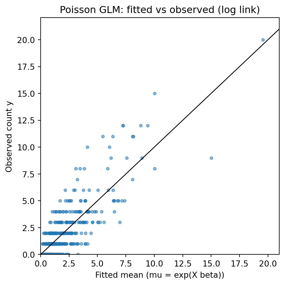
The following example simulates count data with a known log linear mean structure, fits a Poisson GLM by maximum likelihood (which statsmodels solves with IRLS), and plots fitted against observed counts. The fixed seed makes the output reproducible, and the printed coefficients should recover the values used to generate the data.
import numpy as npimport statsmodels.api as smimport matplotlib.pyplot as pltrng = np.random.default_rng(0)# Simulate counts with a known log-linear mean: log(mu) = 0.5 + 0.8*x1 - 0.4*x2n =400x1 = rng.normal(0.0, 1.0, n)x2 = rng.normal(0.0, 1.0, n)beta_true = np.array([0.5, 0.8, -0.4])X = np.column_stack([np.ones(n), x1, x2])mu = np.exp(X @ beta_true)y = rng.poisson(mu)# Fit a Poisson GLM with the canonical log link (solved by IRLS)model = sm.GLM(y, X, family=sm.families.Poisson(link=sm.families.links.Log()))result = model.fit()print("Estimated coefficients:", np.round(result.params, 3))print("Standard errors: ", np.round(result.bse, 3))print("Residual deviance: %.2f on %d df"% (result.deviance, result.df_resid))print("AIC: %.2f"% result.aic)fitted = result.fittedvaluesfig, ax = plt.subplots(figsize=(5, 5))ax.scatter(fitted, y, s=12, alpha=0.5)lims = [0, max(fitted.max(), y.max()) *1.05]ax.plot(lims, lims, color="black", linewidth=1)ax.set_xlabel("Fitted mean (mu = exp(X beta))")ax.set_ylabel("Observed count y")ax.set_title("Poisson GLM: fitted vs observed (log link)")ax.set_xlim(lims)ax.set_ylim(bottom=0)plt.tight_layout()plt.show()
Estimated coefficients: [ 0.456  0.797 -0.382]
Standard errors:        [0.044 0.035 0.033]
Residual deviance:      425.84 on 397 df
AIC:                    1250.11
The diagonal line marks where fitted equals observed. Because the variance of a Poisson grows with the mean, the vertical scatter widens to the right, exactly the mean variance relationship \(V(\mu) = \mu\) that the family encodes. The recovered coefficients sit close to the generating values \((0.5, 0.8, -0.4)\), and exponentiating each one gives a rate ratio: a unit increase in \(x_1\) multiplies the expected count by \(e^{0.8} \approx 2.2\).
usingGLM, DataFrames, Random, DistributionsRandom.seed!(0)# Simulate counts: log(mu) = 0.5 + 0.8*x1 - 0.4*x2n =400x1 =randn(n)x2 =randn(n)mu =exp.(0.5.+0.8.* x1 .-0.4.* x2)y = [rand(Poisson(m)) for m in mu]df =DataFrame(y = y, x1 = x1, x2 = x2)# Fit a Poisson GLM with the canonical log linkmodel =glm(@formula(y ~ x1 + x2), df, Poisson(), LogLink())println(coeftable(model))println("Deviance: ", deviance(model))println("AIC: ", aic(model))
// Illustrative: one IRLS step for a Poisson GLM with the canonical log link.// For production use a crate such as `linregress` or `ndarray-linalg`.// Canonical link: g(mu) = log(mu), g'(mu) = 1/mu, V(mu) = mu.// Working weight w_i = mu_i; working response z_i = eta_i + (y_i - mu_i)/mu_i.fn irls_step( x:&[[f64;3]],// design rows: [1, x1, x2] y:&[f64], beta:&[f64;3],) -> [f64;3] {let n = x.len();// Accumulate X^T W X (3x3) and X^T W z (3).letmut xtwx = [[0.0_f64;3];3];letmut xtwz = [0.0_f64;3];for i in0..n {let eta:f64= (0..3).map(|j| x[i][j] * beta[j]).sum();let mu = eta.exp();// inverse log linklet w = mu;// working weight for Poisson + log linklet z = eta + (y[i] - mu) / mu;// working responsefor a in0..3{ xtwz[a] += x[i][a] * w * z;for b in0..3{ xtwx[a][b] += x[i][a] * w * x[i][b];}}}// Solve xtwx * beta_new = xtwz (omitted: a 3x3 linear solve) solve_3x3(&xtwx,&xtwz)}
95.6 6. Deviance and Goodness of Fit
95.6.1 6.1 Definition
In ordinary regression the residual sum of squares measures lack of fit. The GLM generalization is the deviance, defined by comparing the fitted model to the saturated model, the model that perfectly reproduces the data by giving each observation its own parameter (\(\hat{\mu}_i = y_i\)). Let \(\ell(\hat{\boldsymbol{\mu}})\) be the maximized log likelihood of the fitted model and \(\ell(\mathbf{y})\) that of the saturated model. The deviance is
The quantity \(D / \phi\) is the scaled deviance. Smaller deviance means a fit closer to the data. For the Gaussian family the deviance reduces exactly to the residual sum of squares, confirming that deviance is the honest generalization of that quantity.
95.6.2 6.2 Family specific forms
Each family yields a recognizable deviance. For the Poisson,
These expressions are sums of contributions, one per observation, and the signed square roots of those contributions are the deviance residuals, the GLM analogue of ordinary residuals for diagnostic plots.
95.6.3 6.3 Comparing models
Deviance is most useful for comparing nested models. If model \(A\) is nested in model \(B\), the difference in scaled deviances \(D_A - D_B\) is a likelihood ratio statistic. Under the null hypothesis that the smaller model suffices, it follows asymptotically a chi square distribution with degrees of freedom equal to the difference in the number of parameters,
This is the standard way to test whether a group of covariates contributes to the model, the GLM counterpart of the \(F\) test in linear regression. For models that are not nested, the deviance feeds into information criteria such as \(\mathrm{AIC} = D + 2p\) (up to additive constants), which penalize complexity and allow ranking of non nested candidates.
95.6.4 6.4 Residual deviance as a fit check
The residual deviance of a fitted model, compared against its degrees of freedom, offers a rough overall goodness of fit check. For Poisson and binomial models, where \(\phi = 1\), a residual deviance much larger than the residual degrees of freedom signals overdispersion or a misspecified mean structure, prompting the remedies discussed above. This single diagnostic, available from any GLM fit, is one of the framework’s quiet conveniences.
95.7 7. Practical Considerations
Several issues arise repeatedly in applied work. Separation in logistic regression occurs when a covariate perfectly predicts the outcome, driving coefficients to infinity and IRLS to diverge; penalized likelihood methods such as Firth’s correction restore finite, stable estimates. Choice of link should be guided by both interpretability and fit, and the canonical link is a sensible default but not a mandate. Offsets handle exposure and rate modeling cleanly. And weights allow grouped data, where each row represents many identical cases, to be fit as efficiently as individual records. Throughout, the same IRLS engine and the same deviance based inference apply, so mastering the framework once equips you for an entire family of models rather than a single technique.
The enduring value of the GLM framework is conceptual economy. Rather than memorizing separate recipes for continuous, binary, and count outcomes, you learn one structure with three interchangeable parts. The exponential family supplies the distributions and their variance functions, the link function bridges the constrained mean to an unconstrained linear predictor, IRLS estimates the coefficients and delivers their standard errors in one pass, and deviance measures fit and drives model comparison. This unification, now half a century old, remains a cornerstone of applied statistics and a direct ancestor of the generalized additive models, mixed models, and many machine learning methods that extend it.
95.8 References
Nelder, J. A., and Wedderburn, R. W. M. (1972). Generalized Linear Models. Journal of the Royal Statistical Society, Series A, 135(3), 370 to 384. https://doi.org/10.2307/2344614
McCullagh, P., and Nelder, J. A. (1989). Generalized Linear Models, 2nd edition. Chapman and Hall/CRC. https://doi.org/10.1201/9780203753736
Wedderburn, R. W. M. (1974). Quasi likelihood functions, generalized linear models, and the Gauss Newton method. Biometrika, 61(3), 439 to 447. https://doi.org/10.1093/biomet/61.3.439
Dobson, A. J., and Barnett, A. G. (2018). An Introduction to Generalized Linear Models, 4th edition. Chapman and Hall/CRC. https://doi.org/10.1201/9781315182780
Agresti, A. (2015). Foundations of Linear and Generalized Linear Models. Wiley. ISBN 9781118730034.
Hastie, T., Tibshirani, R., and Friedman, J. (2009). The Elements of Statistical Learning, 2nd edition. Springer. https://doi.org/10.1007/978-0-387-84858-7
Faraway, J. J. (2016). Extending the Linear Model with R, 2nd edition. Chapman and Hall/CRC. https://doi.org/10.1201/9781315382722
Wood, S. N. (2017). Generalized Additive Models: An Introduction with R, 2nd edition. Chapman and Hall/CRC. https://doi.org/10.1201/9781315370279
Source Code
# Generalized Linear ModelsOrdinary least squares regression rests on a comfortable but restrictive set of assumptions: the response is continuous, its conditional mean is a linear function of the predictors, and the noise around that mean is Gaussian with constant variance. A great deal of real data violates these assumptions in obvious ways. Counts of events are nonnegative integers. Binary outcomes live in $\{0, 1\}$. Proportions are bounded between zero and one. Waiting times are positive and skewed. Forcing a linear Gaussian model onto such data produces predictions that fall outside the valid range and standard errors that are simply wrong.Generalized Linear Models, introduced by Nelder and Wedderburn in 1972, provide a single coherent framework that accommodates all of these cases. The key insight is that linear regression, logistic regression, and Poisson regression are not three unrelated techniques but three instances of one model class, differing only in two choices: the probability distribution assumed for the response and the function that connects the linear predictor to the mean. Once you see the unifying structure, a single estimation algorithm fits all of them, a single notion of residual deviance measures fit across all of them, and the asymptotic inference theory transfers wholesale. This chapter develops that structure from the exponential family upward and shows how it pays off in practice.## 1. The Exponential Family### 1.1 Canonical formA distribution belongs to the one parameter exponential family if its density or mass function can be written as$$f(y \mid \theta, \phi) = \exp\!\left\{ \frac{y\theta - b(\theta)}{a(\phi)} + c(y, \phi) \right\}.$$Here $\theta$ is the natural or canonical parameter, $\phi$ is a dispersion parameter, and $a$, $b$, $c$ are known functions that specify the particular distribution. The function $b(\theta)$ is called the cumulant function and it carries all the information we need about the mean and variance.This form looks abstract, but many familiar distributions fit it after light algebra. Consider the Gaussian with known variance $\sigma^2$:$$f(y) = \frac{1}{\sqrt{2\pi\sigma^2}} \exp\!\left\{ -\frac{(y - \mu)^2}{2\sigma^2} \right\}= \exp\!\left\{ \frac{y\mu - \mu^2/2}{\sigma^2} - \frac{y^2}{2\sigma^2} - \frac{1}{2}\log(2\pi\sigma^2) \right\}.$$Matching terms gives $\theta = \mu$, $b(\theta) = \theta^2/2$, $a(\phi) = \sigma^2$, and $c(y, \phi)$ collects the remaining pieces. The Bernoulli, binomial, Poisson, gamma, and inverse Gaussian distributions all admit analogous representations.### 1.2 Mean and variance from the cumulant functionThe cumulant function earns its name because its derivatives generate the moments of $Y$. The derivation is worth carrying out, because it shows that the mean and variance are not separate assumptions but consequences of the canonical form. Begin from the log likelihood of a single observation,$$\ell(\theta) = \log f(y \mid \theta, \phi) = \frac{y\theta - b(\theta)}{a(\phi)} + c(y, \phi),$$and recall two standard score identities that hold for any regular likelihood,$$\mathbb{E}\!\left[\frac{\partial \ell}{\partial \theta}\right] = 0,\qquad\mathbb{E}\!\left[\frac{\partial^2 \ell}{\partial \theta^2}\right] + \mathbb{E}\!\left[\left(\frac{\partial \ell}{\partial \theta}\right)^{\!2}\right] = 0.$$The first follows from differentiating $\int f \, dy = 1$ under the integral sign; the second is the differentiated form of the same identity. The derivatives of $\ell$ are immediate from the canonical form,$$\frac{\partial \ell}{\partial \theta} = \frac{y - b'(\theta)}{a(\phi)},\qquad\frac{\partial^2 \ell}{\partial \theta^2} = -\frac{b''(\theta)}{a(\phi)}.$$Substituting the first derivative into $\mathbb{E}[\partial \ell / \partial \theta] = 0$ gives $\mathbb{E}[y - b'(\theta)] = 0$, hence $\mu = b'(\theta)$. Substituting both derivatives into the second identity gives$$-\frac{b''(\theta)}{a(\phi)} + \frac{\operatorname{Var}[Y]}{a(\phi)^2} = 0\quad\Longrightarrow\quad\operatorname{Var}[Y] = a(\phi)\, b''(\theta).$$So we arrive at two clean identities,$$\mathbb{E}[Y] = \mu = b'(\theta), \qquad \operatorname{Var}[Y] = a(\phi)\, b''(\theta).$$The first identity says the mean is the derivative of the cumulant function with respect to the natural parameter. The second says the variance factors into a dispersion piece $a(\phi)$ and a piece $b''(\theta)$ that depends only on the mean. Because $\mu = b'(\theta)$ is a function of $\theta$ alone, we can express $b''(\theta)$ as a function of $\mu$, which defines the variance function$$V(\mu) = b''(\theta(\mu)).$$The variance function is the signature of a GLM family. For the Gaussian, $b''(\theta) = 1$, so $V(\mu) = 1$ and the variance is constant. For the Poisson, $V(\mu) = \mu$, so variance equals the mean. For the Bernoulli, $V(\mu) = \mu(1 - \mu)$, which vanishes at the extremes and peaks at $\mu = 1/2$. These mean variance relationships are precisely the empirical patterns we observe in counts and binary data, and the exponential family encodes them as a mathematical consequence rather than an ad hoc assumption.Typically $a(\phi) = \phi / w$ where $w$ is a known prior weight, such as the number of binomial trials or a case weight. For the Poisson and binomial the dispersion is fixed at $\phi = 1$; for the Gaussian and gamma it is a free parameter estimated from the data.## 2. The GLM Framework### 2.1 Three componentsA generalized linear model is fully specified by three components.First, a **random component**: the response $Y_i$ given covariates is drawn independently from an exponential family distribution with mean $\mu_i$.Second, a **systematic component**: a linear predictor $\eta_i = \mathbf{x}_i^\top \boldsymbol{\beta}$ combines the covariates through a vector of coefficients $\boldsymbol{\beta}$.Third, a **link function** $g$ that connects the two through $g(\mu_i) = \eta_i$. The link is a smooth, monotone, invertible function, so we can also write $\mu_i = g^{-1}(\eta_i)$, where $g^{-1}$ is sometimes called the mean function or inverse link.The separation of these three components is what gives the framework its flexibility. The random component fixes the variance function and the likelihood. The systematic component keeps the convenience of linearity in the parameters. The link function bridges them and, crucially, lets us map an unbounded linear predictor onto a constrained mean.### 2.2 Why the link mattersSuppose we model counts. The mean $\mu_i$ must be positive, but the linear predictor $\mathbf{x}_i^\top \boldsymbol{\beta}$ ranges over the whole real line. A log link $g(\mu) = \log \mu$ resolves the tension: $\mu_i = \exp(\mathbf{x}_i^\top \boldsymbol{\beta})$ is automatically positive for any $\boldsymbol{\beta}$. For binary data the mean is a probability in $(0, 1)$, and the logit link $g(\mu) = \log\{\mu / (1 - \mu)\}$ maps that interval onto the real line, with the logistic function as its inverse. The link does the work of respecting the natural constraints of the data while preserving a linear structure for the predictors.### 2.3 The canonical linkAmong all valid links, one is distinguished. The canonical link sets the linear predictor equal to the natural parameter, $\eta = \theta$. Equivalently, $g$ is chosen so that $g(\mu) = \theta(\mu) = (b')^{-1}(\mu)$. The canonical links are:| Family | Variance $V(\mu)$ | Canonical link $g(\mu)$ | Mean function ||---|---|---|---|| Gaussian | $1$ | identity, $\mu$ | $\eta$ || Binomial | $\mu(1-\mu)$ | logit, $\log\frac{\mu}{1-\mu}$ | $\frac{1}{1+e^{-\eta}}$ || Poisson | $\mu$ | log, $\log\mu$ | $e^{\eta}$ || Gamma | $\mu^2$ | inverse, $-1/\mu$ | $-1/\eta$ |Canonical links carry several conveniences. The sufficient statistic for $\boldsymbol{\beta}$ becomes $\mathbf{X}^\top \mathbf{y}$, the observed and expected information matrices coincide, and the score equations take a particularly clean form. You are not obligated to use the canonical link, and sometimes another choice fits the science better. The probit link for binary data and the identity link for Poisson rates both have legitimate uses. But the canonical link is the default for good reasons, and we exploit its properties when deriving the estimator below.## 3. Maximum Likelihood Estimation### 3.1 The log likelihood and scoreWe estimate $\boldsymbol{\beta}$ by maximum likelihood. For independent observations the log likelihood is the sum of individual contributions,$$\ell(\boldsymbol{\beta}) = \sum_{i=1}^n \frac{y_i \theta_i - b(\theta_i)}{a_i(\phi)} + c(y_i, \phi).$$To differentiate with respect to $\boldsymbol{\beta}$ we apply the chain rule through the chain $\boldsymbol{\beta} \to \eta_i \to \mu_i \to \theta_i$. Using $\partial \theta_i / \partial \mu_i = 1 / V(\mu_i)$, $\partial \mu_i / \partial \eta_i = 1 / g'(\mu_i)$, and $\partial \eta_i / \partial \boldsymbol{\beta} = \mathbf{x}_i$, the score function works out to$$\frac{\partial \ell}{\partial \boldsymbol{\beta}}= \sum_{i=1}^n \frac{(y_i - \mu_i)}{a_i(\phi)\, V(\mu_i)\, g'(\mu_i)}\, \mathbf{x}_i .$$Setting this to zero gives the estimating equations. Notice the appealing structure: each observation contributes its residual $y_i - \mu_i$, weighted by a term that depends on the variance and the slope of the link, projected onto the covariate vector. Under the canonical link the messy weighting simplifies, and the score equations reduce to $\mathbf{X}^\top (\mathbf{y} - \boldsymbol{\mu}) = \mathbf{0}$, which says the model matches the data in the directions spanned by the covariates.### 3.2 No closed form in generalExcept for the Gaussian identity link case, which recovers ordinary least squares, these equations are nonlinear in $\boldsymbol{\beta}$ because $\mu_i$ depends on $\boldsymbol{\beta}$ through a nonlinear inverse link. There is no closed form solution. We need an iterative numerical method, and the structure of the exponential family hands us a particularly elegant one.## 4. Iteratively Reweighted Least Squares### 4.1 Newton Raphson meets Fisher scoringThe natural way to solve the score equations is Newton Raphson, which iterates$$\boldsymbol{\beta}^{(t+1)} = \boldsymbol{\beta}^{(t)} + \mathbf{H}^{-1} \mathbf{u},$$where $\mathbf{u}$ is the score and $\mathbf{H}$ is the negative Hessian. Fisher scoring replaces the observed Hessian with its expectation, the Fisher information matrix $\mathcal{I} = \mathbb{E}[-\mathbf{H}]$. For GLMs this expectation has a clean form, and under the canonical link the observed and expected Hessians are identical, so the two methods coincide. The Fisher information for a GLM is$$\mathcal{I}(\boldsymbol{\beta}) = \mathbf{X}^\top \mathbf{W} \mathbf{X},$$where $\mathbf{W}$ is a diagonal matrix of weights $w_i = 1 / \{ a_i(\phi)\, V(\mu_i)\, g'(\mu_i)^2 \}$.### 4.2 The working responseThe remarkable fact is that each Fisher scoring step can be rewritten as a weighted least squares regression. To see why, write the Fisher scoring update in full,$$\boldsymbol{\beta}^{(t+1)} = \boldsymbol{\beta}^{(t)} + \mathcal{I}^{-1} \mathbf{u}= \boldsymbol{\beta}^{(t)} + (\mathbf{X}^\top \mathbf{W} \mathbf{X})^{-1} \mathbf{X}^\top \mathbf{W} \mathbf{r},$$where the score from Section 3.1 has been factored as $\mathbf{u} = \mathbf{X}^\top \mathbf{W} \mathbf{r}$ with residual vector entries $r_i = (y_i - \mu_i)\, g'(\mu_i)$. This factorization follows by writing the score weight $1 / \{ a_i(\phi)\, V(\mu_i)\, g'(\mu_i) \}$ as $w_i \cdot g'(\mu_i)$, with $w_i = 1 / \{ a_i(\phi)\, V(\mu_i)\, g'(\mu_i)^2 \}$ matching the Fisher information weights. Now pull the leading $\boldsymbol{\beta}^{(t)}$ inside by noting $\boldsymbol{\beta}^{(t)} = (\mathbf{X}^\top \mathbf{W} \mathbf{X})^{-1} \mathbf{X}^\top \mathbf{W} \mathbf{X} \boldsymbol{\beta}^{(t)}$ and that $\mathbf{X}\boldsymbol{\beta}^{(t)} = \boldsymbol{\eta}$, which gives$$\boldsymbol{\beta}^{(t+1)} = (\mathbf{X}^\top \mathbf{W} \mathbf{X})^{-1} \mathbf{X}^\top \mathbf{W} (\boldsymbol{\eta} + \mathbf{r}).$$The bracketed quantity is the working response, sometimes called the adjusted dependent variable,$$z_i = \eta_i + (y_i - \mu_i)\, g'(\mu_i).$$This is a first order Taylor expansion of the link applied to the data: it linearizes $g(y_i)$ around the current fitted mean. With the weights $w_i$ above, the Fisher scoring update is therefore exactly the solution of a weighted least squares problem,$$\boldsymbol{\beta}^{(t+1)} = (\mathbf{X}^\top \mathbf{W} \mathbf{X})^{-1} \mathbf{X}^\top \mathbf{W} \mathbf{z}.$$Because both the weights $\mathbf{W}$ and the working response $\mathbf{z}$ depend on the current estimate of $\boldsymbol{\beta}$ through $\mu_i$ and $\eta_i$, we recompute them at every iteration. Hence the name: Iteratively Reweighted Least Squares, or IRLS.### 4.3 The algorithmThe procedure is compact and the same code fits every family.The iteratively reweighted least squares (IRLS) procedure is:1. Initialize $\mu$ from the data (often $\mu = y$, lightly adjusted) and set the linear predictor $\eta = g(\mu)$.2. Repeat until convergence: - Working response: $z = \eta + (y - \mu)\,g'(\mu)$ - Working weights: $w = \dfrac{1}{a(\phi)\,V(\mu)\,g'(\mu)^2}$ - Weighted least squares: $\beta = (X^\top W X)^{-1} X^\top W z$, with $W = \operatorname{diag}(w)$ - Update: $\eta = X\beta$, then $\mu = g^{-1}(\eta)$Each iteration is a single weighted regression, which off the shelf linear algebra handles efficiently and stably, for instance through a QR or Cholesky decomposition rather than explicit matrix inversion. Because the GLM log likelihood with a canonical link is concave in $\boldsymbol{\beta}$, IRLS converges to the global maximum from essentially any starting point, usually in a handful of iterations. This is the practical payoff of the exponential family structure: one algorithm, provably well behaved, for the entire model class.### 4.4 Standard errors for freeConvergence yields more than point estimates. The inverse of the Fisher information at the solution, $(\mathbf{X}^\top \mathbf{W} \mathbf{X})^{-1}$ evaluated at $\hat{\boldsymbol{\beta}}$, is the asymptotic covariance matrix of $\hat{\boldsymbol{\beta}}$. Its diagonal square roots are the standard errors. The final $\mathbf{W}$ from IRLS is therefore exactly the object we need for inference, which is why fitting and inference are so tightly integrated in GLM software. Wald tests, confidence intervals, and the large sample normal approximation $\hat{\boldsymbol{\beta}} \approx \mathcal{N}(\boldsymbol{\beta}, (\mathbf{X}^\top \mathbf{W} \mathbf{X})^{-1})$ all follow directly.## 5. Three Models, One Framework### 5.1 Linear regressionChoosing the Gaussian random component with the identity link recovers ordinary least squares. The variance function is constant, $g'(\mu) = 1$, the working response is just $z_i = y_i$, and the weights are constant, so IRLS converges in a single step to the familiar normal equations $\boldsymbol{\beta} = (\mathbf{X}^\top \mathbf{X})^{-1} \mathbf{X}^\top \mathbf{y}$. Linear regression is the degenerate case of the GLM where iteration is unnecessary.### 5.2 Logistic regressionChoosing the binomial random component with the logit link gives logistic regression. Here $\mu_i$ is the probability of success, the mean function is the logistic curve $\mu_i = 1 / (1 + e^{-\eta_i})$, and the variance function is $\mu_i(1 - \mu_i)$. The coefficients have a natural interpretation as log odds ratios: a unit increase in a covariate multiplies the odds of the outcome by $e^{\beta_j}$. IRLS for this model is the standard fitting routine, and the working weights $w_i = \mu_i(1 - \mu_i)$ down weight observations whose predicted probabilities are near zero or one.### 5.3 Poisson regressionChoosing the Poisson random component with the log link gives the standard model for count data. The mean function is $\mu_i = e^{\eta_i}$, guaranteeing positivity, and the variance function is $V(\mu) = \mu$, so the model builds in the count data property that variance grows with the mean. Coefficients are interpreted multiplicatively on the rate scale: $e^{\beta_j}$ is the rate ratio for a unit change in the covariate. When counts arise from exposures of differing sizes, such as accidents per vehicle mile, an offset term $\log(\text{exposure}_i)$ enters the linear predictor with a fixed coefficient of one, turning the model into a rate model.A practical caution: real count data often shows variance exceeding the mean, a phenomenon called overdispersion. The Poisson model cannot represent this because its dispersion is fixed at one. Remedies include estimating a free dispersion parameter via quasi Poisson estimation or switching to the negative binomial distribution, which adds a second parameter to decouple the variance from the mean.### 5.4 Fitting a Poisson GLM in codeThe following example simulates count data with a known log linear mean structure, fits a Poisson GLM by maximum likelihood (which `statsmodels` solves with IRLS), and plots fitted against observed counts. The fixed seed makes the output reproducible, and the printed coefficients should recover the values used to generate the data.::: {.panel-tabset}## Python```{python}import numpy as npimport statsmodels.api as smimport matplotlib.pyplot as pltrng = np.random.default_rng(0)# Simulate counts with a known log-linear mean: log(mu) = 0.5 + 0.8*x1 - 0.4*x2n =400x1 = rng.normal(0.0, 1.0, n)x2 = rng.normal(0.0, 1.0, n)beta_true = np.array([0.5, 0.8, -0.4])X = np.column_stack([np.ones(n), x1, x2])mu = np.exp(X @ beta_true)y = rng.poisson(mu)# Fit a Poisson GLM with the canonical log link (solved by IRLS)model = sm.GLM(y, X, family=sm.families.Poisson(link=sm.families.links.Log()))result = model.fit()print("Estimated coefficients:", np.round(result.params, 3))print("Standard errors: ", np.round(result.bse, 3))print("Residual deviance: %.2f on %d df"% (result.deviance, result.df_resid))print("AIC: %.2f"% result.aic)fitted = result.fittedvaluesfig, ax = plt.subplots(figsize=(5, 5))ax.scatter(fitted, y, s=12, alpha=0.5)lims = [0, max(fitted.max(), y.max()) *1.05]ax.plot(lims, lims, color="black", linewidth=1)ax.set_xlabel("Fitted mean (mu = exp(X beta))")ax.set_ylabel("Observed count y")ax.set_title("Poisson GLM: fitted vs observed (log link)")ax.set_xlim(lims)ax.set_ylim(bottom=0)plt.tight_layout()plt.show()```The diagonal line marks where fitted equals observed. Because the variance of a Poisson grows with the mean, the vertical scatter widens to the right, exactly the mean variance relationship $V(\mu) = \mu$ that the family encodes. The recovered coefficients sit close to the generating values $(0.5, 0.8, -0.4)$, and exponentiating each one gives a rate ratio: a unit increase in $x_1$ multiplies the expected count by $e^{0.8} \approx 2.2$.## Julia```juliausingGLM, DataFrames, Random, DistributionsRandom.seed!(0)# Simulate counts: log(mu) = 0.5 + 0.8*x1 - 0.4*x2n =400x1 =randn(n)x2 =randn(n)mu =exp.(0.5.+0.8.* x1 .-0.4.* x2)y = [rand(Poisson(m)) for m in mu]df =DataFrame(y = y, x1 = x1, x2 = x2)# Fit a Poisson GLM with the canonical log linkmodel =glm(@formula(y ~ x1 + x2), df, Poisson(), LogLink())println(coeftable(model))println("Deviance: ", deviance(model))println("AIC: ", aic(model))```## Rust```rust// Illustrative: one IRLS step for a Poisson GLM with the canonical log link.// For production use a crate such as `linregress` or `ndarray-linalg`.// Canonical link:g(mu) =log(mu), g'(mu) = 1/mu, V(mu) = mu.// Working weight w_i = mu_i; working response z_i = eta_i + (y_i - mu_i)/mu_i.fn irls_step( x: &[[f64; 3]], // design rows: [1, x1, x2] y: &[f64], beta: &[f64; 3],) -> [f64; 3] { let n = x.len(); // Accumulate X^T W X (3x3) and X^T W z (3). let mut xtwx = [[0.0_f64; 3]; 3]; let mut xtwz = [0.0_f64; 3]; for i in 0..n { let eta: f64 = (0..3).map(|j| x[i][j] * beta[j]).sum(); let mu = eta.exp(); // inverse log link let w = mu; // working weight for Poisson + log link let z = eta + (y[i] - mu) / mu; // working response for a in 0..3 { xtwz[a] += x[i][a] * w * z; for b in 0..3 { xtwx[a][b] += x[i][a] * w * x[i][b]; } } } // Solve xtwx * beta_new = xtwz (omitted: a 3x3 linear solve) solve_3x3(&xtwx, &xtwz)}```:::## 6. Deviance and Goodness of Fit### 6.1 DefinitionIn ordinary regression the residual sum of squares measures lack of fit. The GLM generalization is the deviance, defined by comparing the fitted model to the saturated model, the model that perfectly reproduces the data by giving each observation its own parameter ($\hat{\mu}_i = y_i$). Let $\ell(\hat{\boldsymbol{\mu}})$ be the maximized log likelihood of the fitted model and $\ell(\mathbf{y})$ that of the saturated model. The deviance is$$D = 2\,\phi\,\bigl[\ell(\mathbf{y}) - \ell(\hat{\boldsymbol{\mu}})\bigr]= 2 \sum_{i=1}^n w_i \bigl[\, y_i(\theta_i^{\text{sat}} - \hat{\theta}_i) - b(\theta_i^{\text{sat}}) + b(\hat{\theta}_i) \,\bigr].$$The quantity $D / \phi$ is the scaled deviance. Smaller deviance means a fit closer to the data. For the Gaussian family the deviance reduces exactly to the residual sum of squares, confirming that deviance is the honest generalization of that quantity.### 6.2 Family specific formsEach family yields a recognizable deviance. For the Poisson,$$D = 2 \sum_i \left[ y_i \log\frac{y_i}{\hat{\mu}_i} - (y_i - \hat{\mu}_i) \right],$$and for the binomial with $n_i$ trials,$$D = 2 \sum_i \left[ y_i \log\frac{y_i}{\hat{\mu}_i} + (n_i - y_i)\log\frac{n_i - y_i}{n_i - \hat{\mu}_i} \right].$$These expressions are sums of contributions, one per observation, and the signed square roots of those contributions are the deviance residuals, the GLM analogue of ordinary residuals for diagnostic plots.### 6.3 Comparing modelsDeviance is most useful for comparing nested models. If model $A$ is nested in model $B$, the difference in scaled deviances $D_A - D_B$ is a likelihood ratio statistic. Under the null hypothesis that the smaller model suffices, it follows asymptotically a chi square distribution with degrees of freedom equal to the difference in the number of parameters,$$D_A - D_B \;\overset{\cdot}{\sim}\; \chi^2_{p_B - p_A}.$$This is the standard way to test whether a group of covariates contributes to the model, the GLM counterpart of the $F$ test in linear regression. For models that are not nested, the deviance feeds into information criteria such as $\mathrm{AIC} = D + 2p$ (up to additive constants), which penalize complexity and allow ranking of non nested candidates.### 6.4 Residual deviance as a fit checkThe residual deviance of a fitted model, compared against its degrees of freedom, offers a rough overall goodness of fit check. For Poisson and binomial models, where $\phi = 1$, a residual deviance much larger than the residual degrees of freedom signals overdispersion or a misspecified mean structure, prompting the remedies discussed above. This single diagnostic, available from any GLM fit, is one of the framework's quiet conveniences.## 7. Practical ConsiderationsSeveral issues arise repeatedly in applied work. Separation in logistic regression occurs when a covariate perfectly predicts the outcome, driving coefficients to infinity and IRLS to diverge; penalized likelihood methods such as Firth's correction restore finite, stable estimates. Choice of link should be guided by both interpretability and fit, and the canonical link is a sensible default but not a mandate. Offsets handle exposure and rate modeling cleanly. And weights allow grouped data, where each row represents many identical cases, to be fit as efficiently as individual records. Throughout, the same IRLS engine and the same deviance based inference apply, so mastering the framework once equips you for an entire family of models rather than a single technique.The enduring value of the GLM framework is conceptual economy. Rather than memorizing separate recipes for continuous, binary, and count outcomes, you learn one structure with three interchangeable parts. The exponential family supplies the distributions and their variance functions, the link function bridges the constrained mean to an unconstrained linear predictor, IRLS estimates the coefficients and delivers their standard errors in one pass, and deviance measures fit and drives model comparison. This unification, now half a century old, remains a cornerstone of applied statistics and a direct ancestor of the generalized additive models, mixed models, and many machine learning methods that extend it.## References1. Nelder, J. A., and Wedderburn, R. W. M. (1972). Generalized Linear Models. Journal of the Royal Statistical Society, Series A, 135(3), 370 to 384. https://doi.org/10.2307/23446142. McCullagh, P., and Nelder, J. A. (1989). Generalized Linear Models, 2nd edition. Chapman and Hall/CRC. https://doi.org/10.1201/97802037537363. Wedderburn, R. W. M. (1974). Quasi likelihood functions, generalized linear models, and the Gauss Newton method. Biometrika, 61(3), 439 to 447. https://doi.org/10.1093/biomet/61.3.4394. Dobson, A. J., and Barnett, A. G. (2018). An Introduction to Generalized Linear Models, 4th edition. Chapman and Hall/CRC. https://doi.org/10.1201/97813151827805. Agresti, A. (2015). Foundations of Linear and Generalized Linear Models. Wiley. ISBN 9781118730034.6. Hastie, T., Tibshirani, R., and Friedman, J. (2009). The Elements of Statistical Learning, 2nd edition. Springer. https://doi.org/10.1007/978-0-387-84858-77. Faraway, J. J. (2016). Extending the Linear Model with R, 2nd edition. Chapman and Hall/CRC. https://doi.org/10.1201/97813153827228. Wood, S. N. (2017). Generalized Additive Models: An Introduction with R, 2nd edition. Chapman and Hall/CRC. https://doi.org/10.1201/9781315370279