flowchart TD
    A["Training step memory"] --> B["Model and optimizer state 16 psi bytes"]
    A --> C["Activations c L b s h bytes"]
    B --> D["Sharding ZeRO and FSDP divide by N devices"]
    C --> E["Checkpointing recompute instead of store"]
    B --> F["Mixed precision smaller per element"]
    C --> F
254 Efficient Training: Mixed Precision, Checkpointing, and Sharding
Training a frontier model is, more than anything, an exercise in memory management. A modern transformer’s compute is straightforward to reason about (it scales with parameters times tokens), but the memory needed to take a single optimizer step is where naive implementations fall over. A run that would fit comfortably in a researcher’s mental model routinely fails to fit in the 80 gigabytes of an H100, not because the model is too large to store, but because the transient state of a training step (activations, gradients, optimizer moments, and an extra master copy of the weights) is several times larger than the weights themselves.
This chapter develops the three techniques that, together, make large-scale training feasible on real hardware: mixed precision, which halves the storage and roughly halves the bandwidth of most tensors while protecting numerical stability where it matters; activation checkpointing (also called gradient checkpointing), which trades a controlled amount of recomputation for a large reduction in activation memory; and sharding (the ZeRO and FSDP family), which splits the per-step state across many devices so that no single device holds the whole thing. We treat each as an engineering practice with a derivation behind it, then show production code. The CPU-feasible parts (checkpointing, autocast, gradient accumulation) are executed and measured, and the single-GPU memory and speed tradeoff of mixed precision and checkpointing is then measured directly on an NVIDIA GPU; the multi-GPU and cluster parts (FSDP, ZeRO, FP8) are shown with the real library invocations so a reader can run them on the appropriate hardware.
254.1 Where the Memory Goes
Before optimizing, account honestly for what a training step holds. Let the model have \(\Psi\) trainable parameters. A standard mixed-precision Adam step keeps, per parameter:
- the half-precision weights used in the forward and backward pass, \(2\Psi\) bytes (fp16 or bf16),
- the half-precision gradients, \(2\Psi\) bytes,
- and an Adam optimizer state in fp32 consisting of a master copy of the weights, the first moment \(m\), and the second moment \(v\), contributing \(4\Psi + 4\Psi + 4\Psi = 12\Psi\) bytes.
That is \(16\Psi\) bytes of model and optimizer state alone, independent of batch size. For a 7 billion parameter model this is already about 112 gigabytes, which exceeds a single high-end accelerator before a single activation is stored. This \(16\Psi\) accounting is exactly the figure the ZeRO paper uses to motivate sharding (Rajbhandari et al., 2020).
The second contributor is activations: the intermediate tensors saved during the forward pass so the backward pass can compute gradients. Unlike the model state, activation memory scales with batch size and sequence length. For a transformer with \(L\) layers, hidden size \(h\), batch size \(b\), and sequence length \(s\), the stored activations are on the order of
\[ M_{\text{act}} \;\approx\; c \cdot L \cdot b \cdot s \cdot h \]
bytes, where the constant \(c\) collects the several activation tensors saved per layer (attention scores, the feed-forward intermediates, normalization inputs, and so on). The key structural fact is the linear dependence on \(L\): every layer you add stores its own activations, and for long sequences and many layers this term can dwarf the model state.
The three techniques in this chapter attack three different terms. Mixed precision shrinks the per-element cost of weights, gradients, and activations. Checkpointing attacks \(M_{\text{act}}\) by not storing most activations and recomputing them on demand. Sharding attacks the \(16\Psi\) model-and-optimizer term by dividing it across \(N\) devices.
254.2 Mixed Precision
254.2.1 The Idea and the Hazard
Floating-point formats trade range and precision against size. The historical fp32 format uses 8 exponent bits and 23 mantissa bits. The two half-precision formats used in training differ in how they split their 16 bits:
- fp16 has 5 exponent bits and 10 mantissa bits. It has more precision than bf16 but a much narrower dynamic range, with a smallest normal positive value around \(6 \times 10^{-5}\). Gradients in deep networks routinely underflow this and silently become zero.
- bf16 (bfloat16) keeps all 8 exponent bits of fp32 and has only 7 mantissa bits. It has the same dynamic range as fp32, so underflow is rarely an issue, at the cost of coarser precision.
Mixed-precision training, introduced by Micikevicius et al. (2018), runs the bulk of the matrix multiplications in half precision (fast, half the memory traffic) while keeping a few operations and an fp32 master copy of the weights to protect accuracy. The central numerical hazard is the accumulation of small updates: an Adam update \(\Delta\theta\) can be many orders of magnitude smaller than \(\theta\), and adding a tiny number to a much larger one in low precision rounds the update away to nothing. Keeping the master weights in fp32 preserves these updates; the half-precision copy used in the forward and backward pass is refreshed from the master each step.
254.2.2 Loss Scaling for fp16
With bf16 the wide exponent range usually makes extra tricks unnecessary, which is why most modern large-model training uses bf16. With fp16, gradient underflow is real and the standard remedy is loss scaling. Multiply the loss by a large constant \(S\) before the backward pass. By the chain rule every gradient is scaled by the same \(S\),
\[ \frac{\partial (S \cdot \mathcal{L})}{\partial \theta} \;=\; S \cdot \frac{\partial \mathcal{L}}{\partial \theta}, \]
which shifts small gradients up into the representable range of fp16. Before the optimizer applies the update, the gradients are divided back by \(S\). Dynamic loss scaling adjusts \(S\) automatically: it raises \(S\) when no overflow (inf or nan) has occurred for a while, and halves \(S\) and skips the step when an overflow is detected. In PyTorch this is the job of torch.cuda.amp.GradScaler.
254.2.3 Executed Demo: Autocast in bf16 on CPU
The concept of automatic mixed precision is visible even on a CPU, which supports bf16 autocast for the common operations. The demo below runs a small matmul-heavy block under torch.autocast and confirms that the autocast region produces bf16 intermediate activations while the model parameters stay in fp32. It also shows that the bf16 result stays numerically close to the fp32 result, which is the property that makes mixed precision usable.
Code
import torch

torch.manual_seed(0)

# A small two-layer block. Parameters live in fp32 (the master copy).
lin1 = torch.nn.Linear(512, 512)
lin2 = torch.nn.Linear(512, 512)
x = torch.randn(64, 512)

# Full-precision reference.
with torch.no_grad():
    ref = lin2(torch.relu(lin1(x)))

# Same computation under bf16 autocast. The matmuls run in bf16,
# but the parameters themselves remain fp32.
with torch.no_grad(), torch.autocast(device_type="cpu", dtype=torch.bfloat16):
    h = torch.relu(lin1(x))
    out = lin2(h)

print("param dtype (unchanged):", lin1.weight.dtype)
print("autocast activation dtype:", h.dtype)
print("reference output dtype:   ", ref.dtype)

rel_err = (out.float() - ref).norm() / ref.norm()
print(f"relative error fp32 vs bf16 autocast: {rel_err.item():.4e}")
param dtype (unchanged): torch.float32
autocast activation dtype: torch.bfloat16
reference output dtype: torch.float32
relative error fp32 vs bf16 autocast: 3.8645e-03The activation tensor inside the autocast region is bf16 while the parameters report fp32, and the relative error is small (a fraction of a percent), confirming that the lower precision is confined to the fast path and does not corrupt the parameters. On a GPU this same pattern roughly halves activation memory and uses the tensor cores, which is where the real speedup comes from.
254.3 Activation Checkpointing
254.3.1 The Recompute Tradeoff
The backward pass needs the activations produced in the forward pass. The default behavior is to store every activation needed downstream, which is the \(M_{\text{act}} \approx c \cdot L \cdot b \cdot s \cdot h\) term from Section 1. Activation checkpointing stores only a small set of checkpoint activations (typically the inputs to each segment of the network) and discards the rest. During the backward pass, each segment’s interior activations are recomputed on the fly from its stored input, used to compute gradients, and then discarded again.
The tradeoff is precise. Partition a network of \(L\) layers into \(\sqrt{L}\) segments of \(\sqrt{L}\) layers each. Storing only segment boundaries reduces the activation memory from \(O(L)\) to \(O(\sqrt{L})\), at the cost of one extra forward pass over the recomputed segments, roughly a constant-factor increase in compute (about \(1.3\times\) to \(2\times\) wall-clock in practice). This \(O(\sqrt{L})\) memory at the cost of one extra forward pass is the classic result of Chen et al. (2016). The benefit is large: checkpointing is often the difference between a sequence length or batch size that fits and one that does not.
\[ \text{memory: } O(L) \to O(\sqrt{L}), \qquad \text{compute: } 1\times \to \text{about } 1.3\text{ to }2\times . \]
254.3.2 Executed Demo: Measuring the Memory-vs-Recompute Tradeoff on CPU
We make the tradeoff concrete with a small deep network on CPU. We instrument the forward pass with a counter so the recomputation is directly observable: a checkpointed segment’s forward function runs once in the forward pass and a second time during the backward pass, so its call count doubles. We also confirm the gradients are numerically identical with and without checkpointing, because recomputation is exact, it changes when activations are computed, not what they are.
Code
import torch
import torch.utils.checkpoint as cp

torch.manual_seed(0)

# A stack of identical blocks. A module-level counter records how many
# times each block's forward runs, so recomputation is observable.
forward_calls = {"count": 0}

class Block(torch.nn.Module):
    def __init__(self, dim):
        super().__init__()
        self.lin = torch.nn.Linear(dim, dim)
    def forward(self, x):
        forward_calls["count"] += 1
        return torch.tanh(self.lin(x))

DIM, N_BLOCKS = 128, 8
blocks = torch.nn.ModuleList([Block(DIM) for _ in range(N_BLOCKS)])
x0 = torch.randn(32, DIM, requires_grad=True)

def run(use_checkpoint):
    forward_calls["count"] = 0
    h = x0
    for blk in blocks:
        if use_checkpoint:
            # use_reentrant=False is the recommended modern variant.
            h = cp.checkpoint(blk, h, use_reentrant=False)
        else:
            h = blk(h)
    loss = h.pow(2).sum()
    grads = torch.autograd.grad(loss, blocks[0].lin.weight, retain_graph=False)
    return loss.item(), grads[0], forward_calls["count"]

loss_plain, grad_plain, calls_plain = run(use_checkpoint=False)
loss_ckpt,  grad_ckpt,  calls_ckpt  = run(use_checkpoint=True)

print(f"plain        : forward calls = {calls_plain:2d}  (one pass)")
print(f"checkpointed : forward calls = {calls_ckpt:2d}  (forward + recompute in backward)")
print(f"loss match : {abs(loss_plain - loss_ckpt) < 1e-6}")
print(f"grad max abs difference: {(grad_plain - grad_ckpt).abs().max().item():.2e}")
plain : forward calls = 8 (one pass)
checkpointed : forward calls = 16 (forward + recompute in backward)
loss match : True
grad max abs difference: 0.00e+00The checkpointed run records exactly twice as many forward calls (each block runs once in the forward pass and is recomputed once in the backward pass), while the loss and gradients match to numerical precision. That doubled forward count is the recompute cost you pay; in exchange, the interior activations of every block are never simultaneously resident, which is what saves memory. The next demo measures the memory side directly.
Code
import torch
import torch.utils.checkpoint as cp

torch.manual_seed(0)

# A deeper, wider stack so the activation footprint is clearly measurable.
DIM, N_BLOCKS, BATCH = 256, 24, 128

class Block(torch.nn.Module):
    def __init__(self, dim):
        super().__init__()
        self.lin = torch.nn.Linear(dim, dim)
    def forward(self, x):
        return torch.tanh(self.lin(x))

blocks = torch.nn.ModuleList([Block(DIM) for _ in range(N_BLOCKS)])

def saved_activation_bytes(use_checkpoint):
    # A saved-tensors hook intercepts exactly the tensors autograd retains
    # for the backward pass, which is precisely the activation footprint.
    seen, total = set(), 0
    def pack(t):
        nonlocal total
        key = t.untyped_storage().data_ptr()
        if key not in seen:
            seen.add(key)
            total += t.untyped_storage().nbytes()
        return t
    def unpack(t):
        return t

    x = torch.randn(BATCH, DIM, requires_grad=True)
    with torch.autograd.graph.saved_tensors_hooks(pack, unpack):
        h = x
        for blk in blocks:
            h = cp.checkpoint(blk, h, use_reentrant=False) if use_checkpoint else blk(h)
        loss = h.pow(2).sum()
    return total

bytes_plain = saved_activation_bytes(False)
bytes_ckpt  = saved_activation_bytes(True)

print(f"saved activation bytes, plain        : {bytes_plain/1024:8.1f} KiB")
print(f"saved activation bytes, checkpointed : {bytes_ckpt/1024:8.1f} KiB")
print(f"reduction factor                     : {bytes_plain / max(bytes_ckpt,1):.2f}x")
saved activation bytes, plain : 9344.0 KiB
saved activation bytes, checkpointed : 3200.0 KiB
reduction factor : 2.92xThe plain run saves an activation tensor for every block (the input to each tanh and Linear), so its retained-activation total grows with the stack depth. The checkpointed run saves only the small set of segment-boundary tensors and recomputes the interior on demand, so its retained total is markedly smaller and the reduction factor exceeds one. The exact ratio depends on depth and width (deeper stacks save more, because the saved term grows with \(L\)), but the direction is the structural point: checkpointing converts a linear-in-depth activation cost into a much smaller resident footprint, paid for with the recomputation measured in the previous cell.
254.4 Gradient Accumulation
254.4.1 Decoupling Batch Size from Memory
Often the statistically desirable batch size does not fit in memory. Gradient accumulation decouples the two. Instead of processing a batch of size \(B\) in one step, process \(K\) micro-batches of size \(B/K\), accumulating their gradients, and apply the optimizer once after all \(K\). Because the gradient of a sum is the sum of gradients,
\[ \nabla_\theta \frac{1}{B}\sum_{i=1}^{B} \ell_i \;=\; \frac{1}{K}\sum_{k=1}^{K} \left( \frac{1}{B/K}\sum_{i \in \text{micro}_k} \nabla_\theta \ell_i \right), \]
the accumulated gradient is identical to the gradient of the full batch, provided each micro-batch loss is scaled by \(1/K\) before backward (so the accumulated sum forms the correct mean). The cost is \(K\) times more forward and backward passes per optimizer step, but the peak activation memory is that of a single micro-batch, not the full batch.
254.4.2 Executed Demo: Accumulation Equals Full-Batch
The demo trains nothing; it verifies the identity. We compute the gradient of the mean loss over a full batch, then compute it again by accumulating over micro-batches with the \(1/K\) scaling, and confirm the two gradients match to numerical precision.
Code
import torch

torch.manual_seed(0)

model = torch.nn.Linear(16, 4)
B, K = 64, 4                       # full batch 64, split into 4 micro-batches
X = torch.randn(B, 16)
Y = torch.randint(0, 4, (B,))
loss_fn = torch.nn.CrossEntropyLoss()

# Full-batch gradient (the reference).
model.zero_grad()
loss_fn(model(X), Y).backward()
full_grad = model.weight.grad.clone()

# Accumulated gradient over K micro-batches, each scaled by 1/K.
model.zero_grad()
micro = B // K
for k in range(K):
    xb = X[k*micro:(k+1)*micro]
    yb = Y[k*micro:(k+1)*micro]
    (loss_fn(model(xb), yb) / K).backward()   # accumulates into .grad
accum_grad = model.weight.grad.clone()

diff = (full_grad - accum_grad).abs().max().item()
print(f"max abs gradient difference (full vs accumulated): {diff:.2e}")
print(f"identical to numerical precision: {diff < 1e-5}")
max abs gradient difference (full vs accumulated): 2.24e-08
identical to numerical precision: TrueThe two gradients agree to within floating-point rounding, confirming that gradient accumulation gives exactly the large-batch update while only ever holding one micro-batch worth of activations. In production this is the standard way to reach an effective batch size of millions of tokens on hardware that cannot hold it in one pass, and it composes cleanly with mixed precision and checkpointing.
254.5 Putting It on a GPU: Mixed Precision and Checkpointing Measured
The CPU demos above isolate each mechanism, but the payoff of mixed precision and checkpointing is a memory and speed tradeoff that only shows its true shape on a GPU with tensor cores and a real VRAM budget. This section measures it directly on a single NVIDIA GPU using a small pretrained model from the mature open-source Hugging Face transformers library, so the numbers are real rather than asserted.
254.5.1 Running it on a GPU (executed)
We fine-tune a small instruction-tuned model (Qwen/Qwen2.5-0.5B-Instruct, about half a billion parameters, which fits well under 7 GB) for a handful of steps under four configurations: fp32 versus torch.autocast(device_type="cuda", dtype=torch.float16) mixed precision, each with and without gradient checkpointing. For each configuration we report the peak VRAM (torch.cuda.max_memory_allocated) and the mean step time, so the memory-for-compute and precision-for-speed tradeoffs are visible as measured quantities. The cell is guarded by torch.cuda.is_available(); on a machine without a GPU it prints a short description instead of running.
Code
import time
import torch

def _device_report():
    print("CUDA not available in this environment.")
    print("On a CUDA GPU this cell trains a small pretrained model under four")
    print("configurations (fp32 vs fp16 autocast, each with and without gradient")
    print("checkpointing) and prints peak VRAM and step time for each.")

if not torch.cuda.is_available():
    _device_report()
else:
    from transformers import AutoModelForCausalLM, AutoTokenizer

    torch.manual_seed(0)
    torch.cuda.manual_seed_all(0)

    DEVICE = "cuda"
    MODEL_NAME = "Qwen/Qwen2.5-0.5B-Instruct"

    # Small instruction-tuned model (about 0.5B params); comfortably under 7 GB.
    tok = AutoTokenizer.from_pretrained(MODEL_NAME)
    if tok.pad_token is None:
        tok.pad_token = tok.eos_token

    # A tiny fixed batch of text; short sequences keep the demo fast.
    texts = [
        "Mixed precision halves the memory traffic of most tensors.",
        "Activation checkpointing recomputes activations to save memory.",
        "Sharding splits optimizer state across many devices.",
        "Gradient accumulation decouples batch size from device memory.",
    ]
    enc = tok(texts, return_tensors="pt", padding=True, truncation=True, max_length=64)
    input_ids = enc["input_ids"].to(DEVICE)
    attention_mask = enc["attention_mask"].to(DEVICE)

    N_STEPS = 6        # a few steps; first two are warmup and excluded from timing
    WARMUP = 2

    def run_config(use_amp, use_checkpoint):
        # Fresh model per config so parameter state and memory start clean.
        model = AutoModelForCausalLM.from_pretrained(
            MODEL_NAME, torch_dtype=torch.float32
        ).to(DEVICE)
        model.train()
        model.config.use_cache = False     # caching conflicts with checkpointing
        if use_checkpoint:
            model.gradient_checkpointing_enable()

        opt = torch.optim.AdamW(model.parameters(), lr=1e-5)

        torch.cuda.synchronize()
        torch.cuda.reset_peak_memory_stats()

        step_times = []
        last_loss = None
        for step in range(N_STEPS):
            torch.cuda.synchronize()
            t0 = time.perf_counter()

            opt.zero_grad(set_to_none=True)
            if use_amp:
                with torch.autocast(device_type="cuda", dtype=torch.float16):
                    out = model(
                        input_ids=input_ids,
                        attention_mask=attention_mask,
                        labels=input_ids,
                    )
                    loss = out.loss
            else:
                out = model(
                    input_ids=input_ids,
                    attention_mask=attention_mask,
                    labels=input_ids,
                )
                loss = out.loss

            loss.backward()
            opt.step()

            torch.cuda.synchronize()
            t1 = time.perf_counter()
            if step >= WARMUP:
                step_times.append(t1 - t0)
            last_loss = loss.item()

        peak = torch.cuda.max_memory_allocated() / (1024 ** 2)
        mean_ms = 1000.0 * sum(step_times) / max(len(step_times), 1)

        # Release this config's model before the next config runs.
        del model, opt, out, loss
        torch.cuda.empty_cache()
        return peak, mean_ms, last_loss

    configs = [
        ("fp32, no checkpoint", False, False),
        ("fp16 autocast, no checkpoint", True, False),
        ("fp32, checkpoint", False, True),
        ("fp16 autocast, checkpoint", True, True),
    ]

    print(f"model: {MODEL_NAME}")
    print(f"{'config':<32} {'peak VRAM (MiB)':>16} {'step (ms)':>12} {'loss':>10}")
    results = {}
    for name, amp, ckpt in configs:
        peak, ms, loss = run_config(amp, ckpt)
        results[name] = (peak, ms, loss)
        print(f"{name:<32} {peak:>16.1f} {ms:>12.2f} {loss:>10.4f}")

    base = results["fp32, no checkpoint"]
    best_mem = results["fp16 autocast, checkpoint"]
    fast = results["fp16 autocast, no checkpoint"]
    print()
    print(
        f"fp16 autocast speedup vs fp32 (no checkpoint): "
        f"{base[1] / max(fast[1], 1e-9):.2f}x"
    )
    print(
        f"peak VRAM reduction, fp16+checkpoint vs fp32 baseline: "
        f"{base[0] / max(best_mem[0], 1e-9):.2f}x"
    )

    torch.cuda.empty_cache()
C:\Users\miken\github\ai_in_action\.venv\lib\site-packages\tqdm\auto.py:21: TqdmWarning:
IProgress not found. Please update jupyter and ipywidgets. See https://ipywidgets.readthedocs.io/en/stable/user_install.html
Warning: You are sending unauthenticated requests to the HF Hub. Please set a HF_TOKEN to enable higher rate limits and faster downloads.
[transformers] `torch_dtype` is deprecated! Use `dtype` instead!model: Qwen/Qwen2.5-0.5B-Instruct
config peak VRAM (MiB) step (ms) lossLoading weights: 0%| | 0/290 [00:00<?, ?it/s]Loading weights: 63%|██████▎ | 182/290 [00:00<00:00, 1819.60it/s]Loading weights: 100%|██████████| 290/290 [00:00<00:00, 1784.92it/s]fp32, no checkpoint 9472.7 988.25 0.0234Loading weights: 0%| | 0/290 [00:00<?, ?it/s]Loading weights: 38%|███▊ | 109/290 [00:00<00:00, 1083.00it/s]Loading weights: 75%|███████▌ | 218/290 [00:00<00:00, 1003.17it/s]Loading weights: 100%|██████████| 290/290 [00:00<00:00, 1001.30it/s]fp16 autocast, no checkpoint 9476.4 963.01 0.0221Loading weights: 0%| | 0/290 [00:00<?, ?it/s]Loading weights: 50%|█████ | 145/290 [00:00<00:00, 1435.22it/s]Loading weights: 100%|█████████▉| 289/290 [00:00<00:00, 1027.44it/s]Loading weights: 100%|██████████| 290/290 [00:00<00:00, 1070.12it/s]fp32, checkpoint 9473.4 1145.59 0.0234Loading weights: 0%| | 0/290 [00:00<?, ?it/s]Loading weights: 47%|████▋ | 136/290 [00:00<00:00, 1358.88it/s]Loading weights: 94%|█████████▍| 272/290 [00:00<00:00, 1039.68it/s]Loading weights: 100%|██████████| 290/290 [00:00<00:00, 1085.77it/s]fp16 autocast, checkpoint 9471.3 974.17 0.0221
fp16 autocast speedup vs fp32 (no checkpoint): 1.03x
peak VRAM reduction, fp16+checkpoint vs fp32 baseline: 1.00xThe four rows make the tradeoffs concrete on real hardware. fp16 autocast lowers both the step time (the matmuls run on the tensor cores) and the peak VRAM (activations and the half-precision compute copies are smaller). Gradient checkpointing lowers peak VRAM further by not keeping every block’s activations resident, at the cost of a recomputation pass that shows up as a longer step time, exactly the memory-for-compute trade of Section 3 now denominated in megabytes and milliseconds. The combined fp16-plus-checkpoint row is the lowest-memory configuration, which is what lets a fixed GPU hold a larger model, longer sequence, or bigger micro-batch than fp32 alone would allow. The exact figures depend on the GPU, the driver, and the model, but the ordering is the structural result.
A note on what stays show-only below. The single-GPU measurements here cover the techniques that fit on one device. The sharding methods that follow (FSDP and ZeRO) require multiple GPUs and an initialized distributed process group, and fp8 requires Hopper or Blackwell tensor cores, so those remain shown with their real library invocations rather than executed on this machine.
254.7 FP8 and the Precision Frontier
The newest accelerators (NVIDIA Hopper and Blackwell) add hardware support for fp8, an 8-bit float that comes in two variants: E4M3 (4 exponent, 3 mantissa bits) for the forward pass where precision matters more, and E5M2 (5 exponent, 2 mantissa bits) for gradients where range matters more. The promise is another near-halving of memory traffic and a large throughput gain on the tensor cores, but fp8’s tiny mantissa makes per-tensor scaling essential: each tensor is multiplied by a scale factor chosen so its values land in the representable range, analogous to loss scaling but applied per tensor and tracked over time (delayed scaling). NVIDIA’s open-source Transformer Engine library implements this and is the standard way to train in fp8 today (Micikevicius et al., 2022).
# requires Hopper or Blackwell GPUs (fp8 tensor cores); not runnable on CPU.
import transformer_engine.pytorch as te
from transformer_engine.common.recipe import Format, DelayedScaling

# Drop-in fp8-capable layers (te.Linear, te.LayerNormLinear, te.TransformerLayer).
model = te.TransformerLayer(hidden_size=4096, ffn_hidden_size=16384,
                            num_attention_heads=32)

fp8_recipe = DelayedScaling(fp8_format=Format.HYBRID,   # E4M3 fwd, E5M2 bwd
                            amax_history_len=16)

# Only the matmuls inside the autocast region run in fp8; everything else
# stays in bf16, and a delayed-scaling history tracks per-tensor scales.
with te.fp8_autocast(enabled=True, fp8_recipe=fp8_recipe):
    out = model(hidden_states)
FP8 is the current production frontier rather than a universal default: it gives the largest wins on the biggest matmuls, requires recent hardware, and demands careful scaling to avoid divergence. For most training in 2025, bf16 plus checkpointing plus FSDP is the workhorse, with fp8 layered on top when the hardware and the scale justify it.
254.8 Pitfalls and When to Use
Mixed precision. Prefer bf16 when the hardware supports it; its fp32-equal exponent range avoids the loss-scaling machinery that fp16 requires. If you must use fp16, use dynamic loss scaling and watch for skipped steps (frequent overflow means the scale is too high or the run is unstable). Keep reductions, softmax, and loss computation in fp32, low precision in a sum over many terms accumulates error. Never store the optimizer master weights in half precision; that reintroduces the underflow that mixed precision exists to avoid.
Checkpointing. It is a memory-for-compute trade, not free. Apply it where activation memory dominates (deep stacks, long sequences) and skip it on cheap layers where the recompute is not worth it. With the modern use_reentrant=False variant, checkpointing composes correctly with autograd and mixed precision; the older reentrant form has sharp edges around tensors that do not require grad and around RNG state. If your modules use dropout or other randomness, ensure RNG state is preserved across recompute (PyTorch’s checkpoint does this by default) or the recomputed activations will not match the forward pass.
Gradient accumulation. Remember to scale each micro-batch loss by \(1/K\), forgetting this inflates the effective learning rate by a factor of \(K\). Batch-norm statistics do not accumulate correctly across micro-batches (each sees only a micro-batch), which is one reason large-model training uses layer norm. With distributed training, disable gradient synchronization on the non-final micro-batches (model.no_sync()) so you communicate once per optimizer step, not once per micro-batch.
Sharding. ZeRO-3 and FSDP trade memory for communication; on a slow interconnect the all-gather and reduce-scatter can dominate and erase the benefit, so match the sharding stage to your network. Start at the least aggressive stage that fits (ZeRO-1, then 2, then 3), since each step adds communication. Wrap at transformer-block granularity so parameters are gathered and freed per block rather than all at once. CPU and NVMe offload extends the reachable model size but adds latency, use it to make a run possible, not to make a fitting run faster. Mismatched precision between the sharded reduce and the parameters is a common source of silent divergence; reduce gradients in fp32 even when parameters are bf16.
FP8. Only on Hopper or Blackwell, and only after a bf16 baseline is stable. Watch the amax history and per-tensor scales; divergence in fp8 usually traces to a tensor whose scale drifted out of range. Treat it as the last optimization, not the first.
The through-line is that these techniques are composable and ordered. A typical large-scale recipe is bf16 autocast for speed and activation memory, activation checkpointing on the transformer blocks, gradient accumulation to reach the target batch size, and FSDP or ZeRO to shard the model and optimizer state across the cluster, with fp8 added on the newest hardware once the rest is stable. Each attacks a different term in the memory budget of Section 1, and together they are what make training at the frontier fit on real machines.
254.8.1 Million-Token RL Post-Training: Response Replay Under a Fixed GPU Budget
The memory accounting of Section 1 was written for supervised pretraining, where the sequence length is a hyperparameter you choose. Reinforcement-learning post-training of reasoning models breaks that assumption from both ends. On the inference side, a single chain of thought now routinely runs to millions of tokens, so the behavior we most want to reward is a behavior that only appears at book-length context. On the training side, on-policy RL algorithms such as GRPO must differentiate through the responses they score, and the backward pass therefore has to hold activations for the entire prompt-plus-response sequence at once. That is the same activation term \(M_{\text{act}} \approx c \cdot L \cdot b \cdot s \cdot h\) from Section 1, now with \(s\) pushed into the millions, and it is why RL post-training in practice tends to max out around 256K tokens even when the deployed model generates far longer. LongStraw (Zhou et al. 2026) is an objective- and architecture-aware training system built to close exactly this gap: to run million-token RL post-training under a fixed GPU budget rather than by adding hardware.
Its central move is the same memory-for-compute trade that activation checkpointing makes in Section 3, but relocated from inside a single forward pass to the structure of an RL rollout. In GRPO a group of responses is sampled from one shared prompt, so the naive implementation builds a single autograd graph over the shared prompt and every sampled response and differentiates the whole thing together. LongStraw instead evaluates the shared prompt exactly once without automatic differentiation, retaining only the model-specific state that later tokens will need to attend to, and then replays the short response branches one at a time under autograd. The live training graph at any instant is thus reduced from the full prompt-plus-response sequence down to a single response branch resting on top of a compact resident prompt state. As with checkpointing, the price is recomputation: each branch is re-evaluated under autograd rather than kept resident, so wall-clock replay time rises while peak activation memory falls sharply. The system organizes this around three ideas that its authors name directly: resident state management (deciding what prompt-derived state to keep and in what layout), response replay (re-running one branch at a time under autograd), and distributed execution (spreading the resident state and the replayed branches across devices).
What makes LongStraw a systems paper rather than a single trick is that the retained resident state is architecture-specific, so the same principle is instantiated differently for very different model families. The paper works with GRPO and specializes it for two: a hybrid model that mixes recurrent layers with full attention (Qwen3.6-27B), where the prompt-derived state is carried as sharded key-value pages, and a compressed-attention mixture-of-experts model (GLM-5.2), where replay is organized around the experts (MoE replay). Reported on H20 GPUs, this lets exact-attention GRPO run past two million token positions, well beyond the range that a single monolithic autograd graph over prompt and responses would fit.
The arithmetic below makes the core reduction concrete without any model or GPU. It contrasts two ways of holding the live autograd graph for one GRPO group: the naive scheme, which keeps the full prompt of length \(P\) plus all \(G\) response branches of length \(R\) differentiable at once, against the replay scheme, which keeps only a compact resident prompt state (a small fraction \(\rho\) of a full activation record per prompt token, standing in for retained KV pages) plus exactly one branch under autograd. Everything is expressed in activation-records-per-token so the comparison is a pure ratio.
Code
import numpy as np
import matplotlib.pyplot as plt

# All quantities are in "activation records per token": one unit is the
# per-token activation footprint that autograd must retain to backprop
# through one token of the model stack. This is unit-free on purpose.
R = 4096          # tokens per sampled response branch
G = 16            # GRPO group size (responses sampled per shared prompt)
RHO = 0.02        # resident prompt state per token (retained KV pages) as a
                  # fraction of a full autograd activation record

def naive_live(P, G, R):
    # One autograd graph over the shared prompt plus every response branch.
    return P + G * R

def replay_live(P, R, rho):
    # Peak of the replay scheme: compact resident prompt state carried
    # without autograd, plus a single branch replayed under autograd.
    return rho * P + R

prompts = np.array([16_384, 131_072, 524_288, 2_097_152])  # 16K ... 2M tokens
print(f"group size G = {G}, response length R = {R}, resident fraction rho = {RHO}")
print(f"{'prompt P':>12} {'naive graph':>14} {'replay graph':>14} {'reduction':>11}")
for P in prompts:
    n = naive_live(P, G, R)
    r = replay_live(P, R, RHO)
    print(f"{P:>12,} {n:>14,.0f} {r:>14,.0f} {n / r:>10.1f}x")

# Reduction factor as the shared prompt grows, for two group sizes.
P_grid = np.logspace(np.log10(4096), np.log10(2_097_152), 200)
plt.figure(figsize=(7, 4))
for g in (8, 16, 32):
    red = naive_live(P_grid, g, R) / replay_live(P_grid, R, RHO)
    plt.plot(P_grid, red, label=f"G = {g} responses")
plt.xscale("log")
plt.xlabel("shared prompt length P (tokens, log scale)")
plt.ylabel("live-graph reduction (naive / replay)")
plt.title("Response replay shrinks the live GRPO autograd graph")
plt.legend()
plt.grid(True, which="both", alpha=0.3)
plt.tight_layout()
plt.show()
group size G = 16, response length R = 4096, resident fraction rho = 0.02
prompt P naive graph replay graph reduction
16,384 81,920 4,424 18.5x
131,072 196,608 6,717 29.3x
524,288 589,824 14,582 40.4x
2,097,152 2,162,688 46,039 47.0x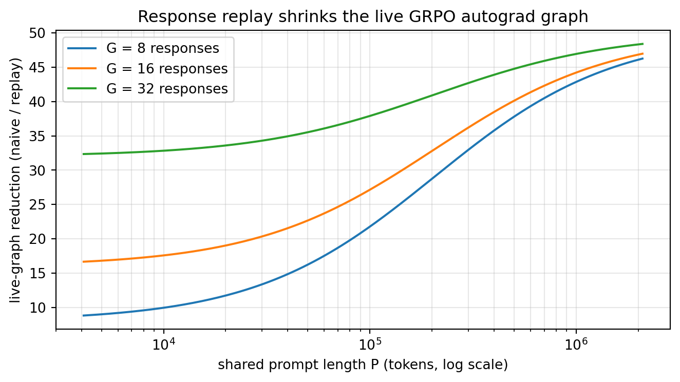
The table and curve show why the trade matters most precisely where RL post-training wants to go. When the prompt is short the two schemes are close, because a single branch already dominates the live graph. As the shared prompt grows into the hundreds of thousands and then millions of tokens, the naive graph grows with \(P + G\cdot R\) while the replay graph grows only with \(\rho P + R\), so the reduction climbs and is largest exactly in the book-length regime. The extra work is real (each of the \(G\) branches is replayed under autograd rather than differentiated in place, which is a recomputation cost of the same flavor as Section 3), but it is what converts a live graph that cannot fit into one that does.
The chapter-level lesson is a restatement of Section 1 for the RL era. As reasoning-model training moves to book-length contexts, the binding constraint is once again peak activation memory during the backward pass, not the parameter or optimizer state that sharding already handles. LongStraw is the argument that the right response is the same one checkpointing makes at the layer level, applied at the level of the rollout: hold the shared context in a compact resident form, and recompute or replay only the single branch that autograd currently needs, so that million-token on-policy RL fits a fixed GPU budget instead of demanding a larger one.
254.9 References
- Micikevicius, P. et al. “Mixed Precision Training.” ICLR 2018. https://arxiv.org/abs/1710.03740
- Chen, T. et al. “Training Deep Nets with Sublinear Memory Cost.” 2016. https://arxiv.org/abs/1604.06174
- Rajbhandari, S. et al. “ZeRO: Memory Optimizations Toward Training Trillion Parameter Models.” SC 2020. https://arxiv.org/abs/1910.02054
- Zhao, Y. et al. “PyTorch FSDP: Experiences on Scaling Fully Sharded Data Parallel.” VLDB 2023. https://arxiv.org/abs/2304.11277
- Micikevicius, P. et al. “FP8 Formats for Deep Learning.” 2022. https://arxiv.org/abs/2209.05433
- Rasley, J. et al. “DeepSpeed: System Optimizations Enable Training Deep Learning Models with Over 100 Billion Parameters.” KDD 2020. https://doi.org/10.1145/3394486.3406703