Most matrices that appear in machine learning are not arbitrary grids of numbers. They carry structure: a covariance matrix is symmetric, a rotation is orthogonal, a kernel Gram matrix is positive semidefinite, and the weight matrix of a graph is sparse. Recognizing and exploiting this structure is one of the most practically valuable skills in applied linear algebra. Structure determines which algorithms apply, how fast they run, how numerically stable they are, and whether a learning problem is even well posed. This chapter surveys the families of special matrices that recur throughout machine learning, the tests that certify membership in each family, and the reasons each structure earns its place in the modeling toolkit.
25.1 1. Symmetric and Hermitian Matrices
25.1.1 1.1 Definitions
A real square matrix \(A \in \mathbb{R}^{n \times n}\) is symmetric when it equals its own transpose:
\[A = A^\top, \qquad \text{equivalently} \qquad a_{ij} = a_{ji} \text{ for all } i, j.\]
The complex generalization replaces the transpose with the conjugate transpose \(A^* = \bar{A}^\top\). A matrix is Hermitian when \(A = A^*\), meaning \(a_{ij} = \overline{a_{ji}}\). Real symmetric matrices are exactly the real Hermitian matrices, so the two notions coincide whenever the entries are real. The diagonal of a Hermitian matrix is always real, since \(a_{ii} = \overline{a_{ii}}\).
25.1.2 1.2 The Spectral Theorem
Symmetry is far more than a notational convenience. The spectral theorem states that every real symmetric matrix admits an orthonormal eigenbasis: there exists an orthogonal matrix \(Q\) and a real diagonal matrix \(\Lambda\) such that
The eigenvalues \(\lambda_i\) are all real, and eigenvectors \(q_i\) corresponding to distinct eigenvalues are orthogonal. For Hermitian matrices the analogous decomposition is \(A = U \Lambda U^*\) with \(U\) unitary and \(\Lambda\) real. No general matrix enjoys such a clean guarantee. The eigenvalues of an arbitrary real matrix can be complex, and its eigenvectors need not be orthogonal or even form a basis. Symmetry removes all of these pathologies at once, which is why so much of machine learning quietly arranges for the matrices it cares about to be symmetric.
The two foundational claims of the spectral theorem deserve short proofs, because they are simple, instructive, and explain exactly where symmetry does its work.
Eigenvalues of a real symmetric matrix are real. Let \(A = A^\top\) be real and let \(\lambda\) be an eigenvalue with (possibly complex) eigenvector \(v \ne 0\), so \(A v = \lambda v\). Take the conjugate transpose of \(A v = \lambda v\) and use \(A^* = A\) (a real symmetric matrix is Hermitian) to get \(v^* A = \bar{\lambda}\, v^*\). Now form the scalar \(v^* A v\) in two ways. Multiplying \(A v = \lambda v\) on the left by \(v^*\) gives \(v^* A v = \lambda\, v^* v\). Multiplying \(v^* A = \bar{\lambda}\, v^*\) on the right by \(v\) gives \(v^* A v = \bar{\lambda}\, v^* v\). Subtracting,
\[(\lambda - \bar{\lambda})\, v^* v = 0.\]
Since \(v \ne 0\), the norm \(v^* v = \|v\|^2 > 0\), so \(\lambda = \bar{\lambda}\), which means \(\lambda\) is real. Because the eigenvalues are real, the eigenvectors can be taken real as well, found in the real null space of \(A - \lambda I\). \(\blacksquare\)
Eigenvectors for distinct eigenvalues are orthogonal. Suppose \(A v_1 = \lambda_1 v_1\) and \(A v_2 = \lambda_2 v_2\) with \(\lambda_1 \ne \lambda_2\), all real. Then
\[\lambda_1\, v_1^\top v_2 = (A v_1)^\top v_2 = v_1^\top A^\top v_2 = v_1^\top A v_2 = \lambda_2\, v_1^\top v_2,\]
where the middle equality uses \(A^\top = A\). Rearranging gives \((\lambda_1 - \lambda_2)\, v_1^\top v_2 = 0\), and since \(\lambda_1 \ne \lambda_2\) we conclude \(v_1^\top v_2 = 0\). When an eigenvalue is repeated, the eigenvectors within its eigenspace can be orthonormalized by the Gram-Schmidt process, so an orthonormal eigenbasis exists in every case. Collecting these orthonormal eigenvectors as the columns of \(Q\) and the eigenvalues on the diagonal of \(\Lambda\) yields \(A = Q \Lambda Q^\top\). \(\blacksquare\)
25.1.3 1.3 Why This Matters in Machine Learning
The covariance matrix of a random vector \(x \in \mathbb{R}^d\),
is symmetric by construction, because \((uv^\top)^\top = vu^\top\) forces the outer-product structure to be self-transposing. Principal component analysis diagonalizes the empirical covariance, and the spectral theorem guarantees that the principal directions are mutually orthogonal and the explained variances (eigenvalues) are real and nonnegative. Hessian matrices of twice-differentiable loss functions are symmetric by the equality of mixed partial derivatives, so second-order optimization methods inherit real eigenvalues that classify critical points as minima, maxima, or saddles. Graph Laplacians, kernel Gram matrices, and the attention-style similarity matrices that arise in many architectures are all symmetric, and algorithms exploit this to halve storage and to use specialized eigensolvers that are both faster and more stable than their general-purpose counterparts.
25.2 2. Orthogonal and Unitary Matrices
25.2.1 2.1 Definitions and Geometric Meaning
A real square matrix \(Q\) is orthogonal when its transpose is its inverse:
\[Q^\top Q = Q Q^\top = I.\]
Equivalently, the columns of \(Q\) form an orthonormal set: each has unit length and any two distinct columns are orthogonal. The complex analog is a unitary matrix \(U\) satisfying \(U^* U = U U^* = I\). Geometrically, orthogonal transformations are exactly the linear maps that preserve inner products, and therefore lengths and angles:
They are the rigid motions of Euclidean space: rotations (when \(\det Q = +1\)) and reflections (when \(\det Q = -1\)). The set of \(n \times n\) orthogonal matrices forms a group under multiplication, the orthogonal group \(O(n)\).
25.2.2 2.2 Key Properties
Every eigenvalue of an orthogonal or unitary matrix has absolute value \(1\), so its action neither amplifies nor shrinks any direction. The determinant is \(\pm 1\), and the condition number with respect to the spectral norm is exactly \(1\), the best possible. This last fact is the deep reason orthogonal matrices are prized in numerical computation: multiplying by \(Q\) cannot amplify rounding error, because \(\|Qx\|_2 = \|x\|_2\) for every vector \(x\). Algorithms built on orthogonal transformations, such as the QR decomposition and the Householder and Givens methods, are numerically stable for precisely this reason.
Orthogonal transformations preserve norms. This is immediate from the defining identity \(Q^\top Q = I\). For any vector \(x\),
\[\|Qx\|_2^2 = (Qx)^\top (Qx) = x^\top Q^\top Q\, x = x^\top I\, x = x^\top x = \|x\|_2^2,\]
so \(\|Qx\|_2 = \|x\|_2\). The converse holds too: if a linear map preserves the norm of every vector, it preserves every inner product through the polarization identity \(\langle x, y \rangle = \tfrac{1}{4}\big(\|x+y\|^2 - \|x-y\|^2\big)\), and a map preserving all inner products must satisfy \(Q^\top Q = I\), hence is orthogonal. Norm preservation and orthogonality are therefore the same property. The eigenvalue claim follows quickly: if \(Qv = \lambda v\) with \(v \ne 0\), then \(\|v\| = \|Qv\| = |\lambda|\,\|v\|\), forcing \(|\lambda| = 1\). \(\blacksquare\)
25.2.3 2.3 Why This Matters in Machine Learning
Orthogonality controls how signals propagate through computation. In deep networks, repeated multiplication by weight matrices can cause activations and gradients to explode or vanish; if the relevant transformations are close to orthogonal, their singular values stay near \(1\) and signal energy is preserved across layers. This motivates orthogonal weight initialization and orthogonal regularization, which penalize departures of \(W^\top W\) from the identity. Recurrent and normalizing-flow models use orthogonal or unitary recurrent maps to keep long-range gradients well conditioned. The QR decomposition \(A = QR\) underlies stable least-squares solvers used in linear regression, and the singular value decomposition \(A = U \Sigma V^\top\), with orthogonal \(U\) and \(V\), is the workhorse behind low-rank approximation, latent semantic analysis, and modern matrix-factorization recommenders. Rotations of coordinate frames in computer vision and robotics are represented by orthogonal matrices precisely because they preserve the geometry of the scene.
25.3 3. Positive Definite and Positive Semidefinite Matrices
25.3.1 3.1 Definitions
Let \(A\) be a real symmetric matrix. We call \(A\)positive semidefinite (PSD), written \(A \succeq 0\), when the associated quadratic form is never negative:
\[x^\top A x \ge 0 \quad \text{for all } x \in \mathbb{R}^n.\]
We call \(A\)positive definite (PD), written \(A \succ 0\), when the form is strictly positive for every nonzero vector:
\[x^\top A x > 0 \quad \text{for all } x \ne 0.\]
Negative definite and negative semidefinite matrices are defined by reversing the inequalities, and an indefinite matrix produces both positive and negative values of the quadratic form. Definiteness is a property of symmetric matrices; for a nonsymmetric matrix one typically applies these notions to its symmetric part \(\tfrac{1}{2}(A + A^\top)\).
25.3.2 3.2 Equivalent Characterizations and Tests
Several conditions are equivalent for a real symmetric matrix, and each gives a practical test:
Eigenvalue test.\(A \succ 0\) if and only if every eigenvalue \(\lambda_i > 0\); \(A \succeq 0\) if and only if every \(\lambda_i \ge 0\). This is the most conceptual characterization but the most expensive to compute.
Cholesky test.\(A \succ 0\) if and only if it admits a Cholesky factorization \(A = L L^\top\) with \(L\) lower triangular and strictly positive diagonal entries. Attempting the factorization and watching for a nonpositive pivot is the fastest reliable numerical check, costing about \(\tfrac{1}{3} n^3\) operations.
Leading minors (Sylvester’s criterion).\(A \succ 0\) if and only if all \(n\) leading principal minors are positive. For semidefiniteness one must check all principal minors, not merely the leading ones.
Gram structure.\(A \succeq 0\) if and only if \(A = B^\top B\) for some matrix \(B\). The matrix is positive definite exactly when \(B\) has full column rank.
The Gram characterization is the one that connects most directly to machine learning, because so many matrices of interest are manifestly of the form \(B^\top B\).
Why the eigenvalue and Gram tests agree. It is worth seeing why these characterizations describe the same matrices. Suppose first that \(A \succeq 0\) in the quadratic-form sense and let \((\lambda, v)\) be an eigenpair with \(\|v\| = 1\). Then
\[\lambda = \lambda\, v^\top v = v^\top (\lambda v) = v^\top A v \ge 0,\]
so every eigenvalue is nonnegative. Conversely, suppose every eigenvalue is nonnegative. Using the spectral decomposition \(A = Q \Lambda Q^\top\) from Section 1, write \(y = Q^\top x\) and expand the quadratic form in the eigenbasis:
\[x^\top A x = x^\top Q \Lambda Q^\top x = y^\top \Lambda y = \sum_{i=1}^{n} \lambda_i\, y_i^2 \ge 0,\]
which is a sum of nonnegative terms. The form is strictly positive for all \(x \ne 0\) exactly when every \(\lambda_i > 0\), giving the positive definite case. The same decomposition supplies the Gram factorization: with \(\lambda_i \ge 0\) we may take square roots and set \(B = \Lambda^{1/2} Q^\top\), where \(\Lambda^{1/2} = \operatorname{diag}(\sqrt{\lambda_1}, \dots, \sqrt{\lambda_n})\). Then
so any PSD matrix is a Gram matrix, and conversely \(x^\top (B^\top B) x = \|Bx\|^2 \ge 0\) shows every \(B^\top B\) is PSD. The eigenvalue test, the Gram test, and the quadratic-form definition are thus three views of one structure. \(\blacksquare\)
25.3.3 3.3 The Covariance Matrix as the Canonical PSD Object
The covariance matrix is the example where all of this structure converges, and it is worth treating explicitly. For a random vector \(x \in \mathbb{R}^d\) with mean \(\mu = \mathbb{E}[x]\), the covariance is \(\Sigma = \mathbb{E}[(x - \mu)(x - \mu)^\top]\). To see that \(\Sigma\) is PSD directly from the definition, fix any direction \(w \in \mathbb{R}^d\) and compute the variance of the scalar projection \(w^\top x\):
The quadratic form \(w^\top \Sigma w\) literally is the variance of the data projected onto \(w\), and a variance can never be negative, so \(\Sigma \succeq 0\) with no further assumptions. The form equals zero only when \(w^\top x\) is constant almost surely, that is, when the data lie in an affine subspace orthogonal to \(w\); ruling out such degenerate directions makes \(\Sigma\) positive definite. The empirical covariance \(\hat{\Sigma} = \tfrac{1}{n} X_c^\top X_c\), where \(X_c\) is the centered data matrix, is manifestly of Gram form \(B^\top B\) with \(B = X_c / \sqrt{n}\), which is a second, purely algebraic proof of the same fact. This single object ties together every theme of the chapter: it is symmetric, so PCA can diagonalize it with a stable eigensolver; its eigenvalues are the principal-direction variances; its Cholesky factor generates Gaussian samples; and its positive definiteness is exactly the condition under which the Gaussian density and the Mahalanobis distance \(\sqrt{(x-\mu)^\top \Sigma^{-1} (x-\mu)}\) are well defined.
We verify positive definiteness by all three tests. Sylvester’s criterion: the leading minors are \(2 > 0\) and \(\det A = 2 \cdot 2 - 1 \cdot 1 = 3 > 0\), so \(A \succ 0\). Eigenvalue test: solving \(\det(A - \lambda I) = (2 - \lambda)^2 - 1 = 0\) gives \(2 - \lambda = \pm 1\), hence \(\lambda_1 = 3\) and \(\lambda_2 = 1\), both positive. The corresponding unit eigenvectors are \(q_1 = \tfrac{1}{\sqrt{2}}(1, 1)^\top\) and \(q_2 = \tfrac{1}{\sqrt{2}}(1, -1)^\top\), which are orthogonal exactly as the spectral theorem predicts for distinct eigenvalues. Cholesky test: seeking \(A = L L^\top\) with \(L = \left[\begin{smallmatrix} \ell_{11} & 0 \\ \ell_{21} & \ell_{22} \end{smallmatrix}\right]\) gives \(\ell_{11} = \sqrt{2}\), then \(\ell_{21} = 1/\sqrt{2}\), and finally \(\ell_{22}^2 = 2 - \tfrac{1}{2} = \tfrac{3}{2}\), so \(\ell_{22} = \sqrt{3/2}\) is real and positive. All three pivots are positive, confirming \(A \succ 0\). The quadratic form expands to \(x^\top A x = 2x_1^2 + 2x_1 x_2 + 2x_2^2 = (x_1 + x_2)^2 + x_1^2 + x_2^2\), visibly a sum of squares and therefore positive for every \(x \ne 0\). Geometrically, the level set \(x^\top A x = 1\) is an ellipse whose axes point along \(q_1\) and \(q_2\) with half-lengths \(1/\sqrt{\lambda_1} = 1/\sqrt{3}\) and \(1/\sqrt{\lambda_2} = 1\).
25.3.5 3.5 Why This Matters in Machine Learning
Positive definiteness is the algebraic signature of convexity and of valid similarity. A twice-differentiable function is convex precisely when its Hessian is positive semidefinite everywhere, and strictly convex when the Hessian is positive definite. Convex losses have a unique global minimum and are tractable to optimize, which is why so much of classical machine learning is engineered to be convex. Covariance matrices are PSD because \(\Sigma = \mathbb{E}[(x-\mu)(x-\mu)^\top]\) has Gram structure, and they are positive definite when no linear combination of features is deterministically constant. A Gaussian density is only well defined when its covariance is positive definite, since the density involves \(\Sigma^{-1}\) and \(\det \Sigma\).
The theory of kernels rests entirely on this structure. A function \(k(x, x')\) is a valid kernel exactly when every Gram matrix \(K_{ij} = k(x_i, x_j)\) it produces is positive semidefinite, by Mercer’s theorem. This guarantees that the kernel corresponds to an inner product in some feature space, which is what makes support vector machines and Gaussian processes well posed. When a Gram matrix loses positive definiteness through rounding, practitioners add a small ridge \(\lambda I\), a transformation that shifts every eigenvalue up by \(\lambda\) and restores a safe margin of positivity. This same trick stabilizes the normal equations \((X^\top X + \lambda I)w = X^\top y\) of ridge regression, where \(X^\top X\) is PSD and the ridge guarantees invertibility.
25.4 4. Diagonal and Triangular Matrices
25.4.1 4.1 Diagonal Matrices
A diagonal matrix \(D\) has \(d_{ij} = 0\) whenever \(i \ne j\). Diagonal matrices are the simplest nontrivial linear maps: they scale each coordinate axis independently by the corresponding diagonal entry. They commute with one another, their product and sum are again diagonal, the inverse (when it exists) is obtained by reciprocating each diagonal entry, and the determinant is the product of the diagonal. Multiplying an \(n \times n\) matrix by a diagonal matrix costs \(O(n^2)\) rather than \(O(n^3)\), because it merely rescales rows or columns.
In machine learning, diagonal matrices encode per-feature scaling and per-coordinate variances. Feature standardization is multiplication by a diagonal matrix of inverse standard deviations. A diagonal covariance assumption (used in naive Bayes and in many variational posteriors) treats features as uncorrelated, trading expressiveness for a dramatic reduction in parameters from \(O(d^2)\) to \(O(d)\). Adaptive optimizers such as Adagrad, RMSProp, and Adam maintain a diagonal preconditioner, approximating the curvature of the loss by a vector of per-parameter scales rather than a full matrix that would be infeasible to store.
25.4.2 4.2 Triangular Matrices
A matrix is lower triangular when all entries above the main diagonal are zero, and upper triangular when all entries below it are zero. Triangular structure is the computational sweet spot of linear algebra: a triangular system \(Lx = b\) is solved directly by forward or backward substitution in \(O(n^2)\) operations, with no need for general elimination. The determinant of a triangular matrix is the product of its diagonal entries, and the product of two lower triangular matrices is lower triangular.
Triangular matrices arise as the outputs of the decompositions that power numerical machine learning. LU decomposition factors a matrix into lower and upper triangular pieces to solve linear systems efficiently. Cholesky decomposition\(A = LL^\top\) produces a single triangular factor for symmetric positive definite matrices and is the standard route to sampling from a multivariate Gaussian: if \(z\) is a standard normal vector, then \(\mu + Lz\) has covariance \(LL^\top = \Sigma\). QR decomposition pairs an orthogonal factor with an upper triangular one to solve least squares stably. In normalizing flows, triangular Jacobians are deliberately engineered so that the log-determinant needed for the change-of-variables formula reduces to a cheap sum of logged diagonal entries.
25.5 5. Sparse Matrices
25.5.1 5.1 What Sparsity Means
A matrix is sparse when the overwhelming majority of its entries are zero, so that the number of nonzeros \(\text{nnz}(A)\) is far smaller than \(n^2\). Sparsity is a property of representation as much as of mathematics: a sparse matrix is stored in formats such as compressed sparse row (CSR), compressed sparse column (CSC), or coordinate list (COO) that record only the nonzero values and their positions. Storage and many operations then scale with \(\text{nnz}(A)\) rather than with \(n^2\). A sparse matrix-vector product, the central operation of iterative solvers, costs \(O(\text{nnz}(A))\), which can be orders of magnitude cheaper than the \(O(n^2)\) dense cost.
25.5.2 5.2 Why This Matters in Machine Learning
Sparsity is pervasive because real data is mostly absences. A bag-of-words or TF-IDF document-term matrix is sparse because any single document uses a tiny fraction of the vocabulary. A user-item interaction matrix in a recommender system is sparse because each user rates a vanishing fraction of the catalog, and the entire enterprise of collaborative filtering is the art of completing this sparse matrix with a low-rank model. One-hot and categorical encodings produce highly sparse design matrices. Graph adjacency matrices are sparse whenever the average degree is small relative to the number of nodes, and graph neural networks lean on sparse matrix multiplication to propagate information along edges at scale.
Sparsity also appears as a modeling goal rather than a given. \(\ell_1\) regularization (the Lasso) drives weight vectors toward sparsity, performing automatic feature selection and yielding models that are smaller, faster, and easier to interpret. Pruning of neural networks removes near-zero weights to produce sparse layers that reduce memory and inference cost. In each case the payoff is the same: exploiting structure to turn an intractable dense computation into a tractable sparse one. Care is required, however, because operations such as matrix inversion or LU factorization can introduce fill-in, converting zeros into nonzeros and destroying the sparsity that motivated the format. Specialized reordering and sparse-direct solvers exist precisely to limit this fill-in.
25.6 6. Special Matrices in Code
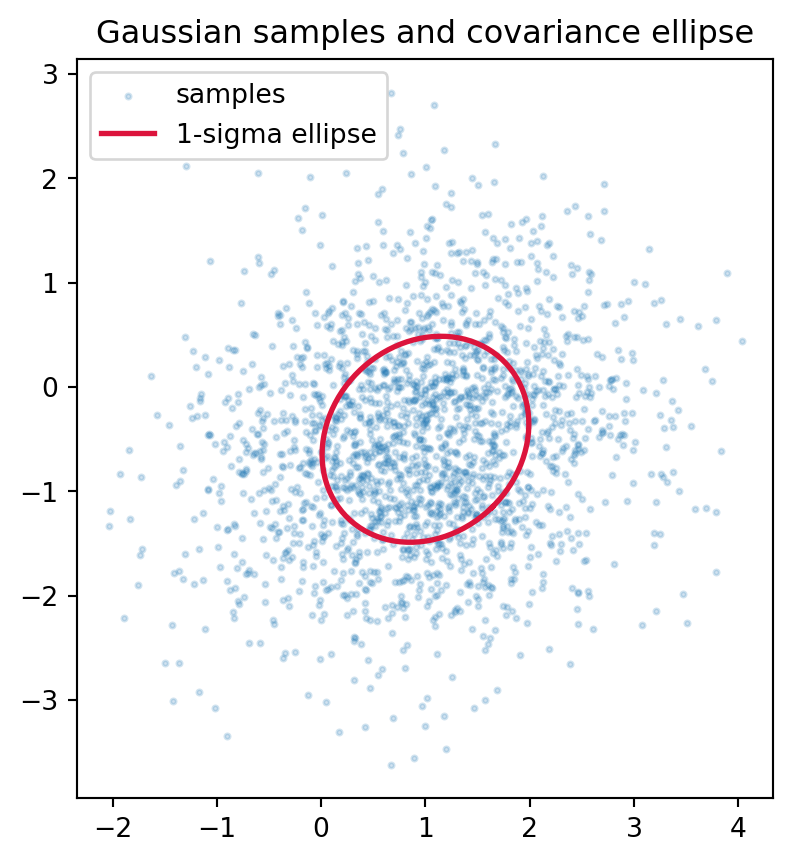
The properties above are most convincing when you can sample a matrix, test it, and watch the geometry appear. The following examples sample an empirical covariance matrix, confirm that it is symmetric and positive definite by both the eigenvalue and Cholesky tests, draw samples from the corresponding Gaussian, and overlay the one-sigma confidence ellipse derived from the eigendecomposition. The Python cell is executable; the Julia and Rust versions are illustrative and show how the same logic reads in each language.
usingLinearAlgebra, RandomRandom.seed!(42)d, n =2, 500B =randn(n, d)Sigma = (B'* B) / n # empirical covariance, PSD by constructionmu = [1.0, -0.5]evals =eigvals(Symmetric(Sigma))is_pd_eig =all(evals .>0)# cholesky throws PosDefException unless strictly positive definite.chol =cholesky(Symmetric(Sigma); check =false)is_pd_chol =issuccess(chol)L = chol.Lprintln("Sigma = ", round.(Sigma, digits =4))println("eigenvalues = ", round.(evals, digits =4))println("PD via eigenvalues = ", is_pd_eig)println("PD via Cholesky = ", is_pd_chol)# Sample from N(mu, Sigma): mu .+ L * z has covariance L L^T.z =randn(d, 2000)samples = mu .+ L * z
// Illustrative: uses the nalgebra crate.// nalgebra = "0.33", rand = "0.8", rand_distr = "0.4"usenalgebra::{DMatrix, DVector};userand::{rngs::StdRng, SeedableRng};userand_distr::{Distribution, StandardNormal};fn main() {letmut rng =StdRng::seed_from_u64(42);let (d, n) = (2usize,500usize);// Empirical covariance Sigma = B^T B / n is PSD by construction.let b =DMatrix::from_fn(n, d,|_, _| StandardNormal.sample(&mut rng));let sigma = (b.transpose() *&b) / (n asf64);// Symmetric eigendecomposition: all eigenvalues must be positive.let eig = sigma.clone().symmetric_eigen();let is_pd_eig = eig.eigenvalues.iter().all(|&l| l >0.0);// Cholesky succeeds iff the matrix is strictly positive definite.let chol = sigma.clone().cholesky();let is_pd_chol = chol.is_some();println!("PD via eigenvalues = {is_pd_eig}");println!("PD via Cholesky = {is_pd_chol}");// Sample from N(mu, Sigma): mu + L z has covariance L L^T.ifletSome(c) = chol {let l = c.l();let mu =DVector::from_vec(vec![1.0,-0.5]);let z =DVector::from_fn(d,|_, _| StandardNormal.sample(&mut rng));let _sample =&mu + l * z;}}
25.7 7. Putting Structure to Work
The families surveyed here overlap and reinforce one another. A covariance matrix is symmetric, positive semidefinite, and often dense; the orthogonal matrix from its spectral decomposition rotates data into principal coordinates; the diagonal matrix of eigenvalues records the variances; a Cholesky factor of the covariance is triangular and generates Gaussian samples; and the design matrix that produced the covariance may itself have been sparse. Each structure narrows the space of possible behaviors and unlocks an algorithm tailored to exploit it.
The practical lesson is to ask, of any matrix encountered in a learning pipeline, what structure it carries and what that structure permits. Is it symmetric, so that a stable eigensolver applies and the eigenvalues are real? Is it positive definite, so that the underlying optimization is convex and a Cholesky factorization will succeed? Is it orthogonal, so that it preserves norms and will not amplify error? Is it sparse, so that linear-time operations replace quadratic ones? The answers determine not only computational cost but also whether the model is well posed at all. Structure is not an incidental property of the matrices in machine learning. It is the reason the field’s core computations remain feasible, stable, and meaningful at scale.
25.8 References
Strang, G. Introduction to Linear Algebra, 6th edition. Wellesley-Cambridge Press, 2023. ISBN 978-1733146678. https://math.mit.edu/~gs/linearalgebra/
Trefethen, L. N., and Bau, D. Numerical Linear Algebra. SIAM, 1997. DOI: 10.1137/1.9780898719574.
Golub, G. H., and Van Loan, C. F. Matrix Computations, 4th edition. Johns Hopkins University Press, 2013. DOI: 10.56021/9781421407944.
Boyd, S., and Vandenberghe, L. Convex Optimization. Cambridge University Press, 2004. DOI: 10.1017/CBO9780511804441.
Horn, R. A., and Johnson, C. R. Matrix Analysis, 2nd edition. Cambridge University Press, 2012. DOI: 10.1017/CBO9781139020411.
Bhatia, R. Positive Definite Matrices. Princeton University Press, 2007. DOI: 10.1515/9781400827787.
Goodfellow, I., Bengio, Y., and Courville, A. Deep Learning, chapter 2 (Linear Algebra). MIT Press, 2016. ISBN 978-0262035613. https://www.deeplearningbook.org/contents/linear_algebra.html
Rasmussen, C. E., and Williams, C. K. I. Gaussian Processes for Machine Learning. MIT Press, 2006. DOI: 10.7551/mitpress/3206.001.0001.
Saad, Y. Iterative Methods for Sparse Linear Systems, 2nd edition. SIAM, 2003. DOI: 10.1137/1.9780898718003.
Source Code
# Special MatricesMost matrices that appear in machine learning are not arbitrary grids of numbers. They carry structure: a covariance matrix is symmetric, a rotation is orthogonal, a kernel Gram matrix is positive semidefinite, and the weight matrix of a graph is sparse. Recognizing and exploiting this structure is one of the most practically valuable skills in applied linear algebra. Structure determines which algorithms apply, how fast they run, how numerically stable they are, and whether a learning problem is even well posed. This chapter surveys the families of special matrices that recur throughout machine learning, the tests that certify membership in each family, and the reasons each structure earns its place in the modeling toolkit.## 1. Symmetric and Hermitian Matrices### 1.1 DefinitionsA real square matrix $A \in \mathbb{R}^{n \times n}$ is **symmetric** when it equals its own transpose:$$A = A^\top, \qquad \text{equivalently} \qquad a_{ij} = a_{ji} \text{ for all } i, j.$$The complex generalization replaces the transpose with the conjugate transpose $A^* = \bar{A}^\top$. A matrix is **Hermitian** when $A = A^*$, meaning $a_{ij} = \overline{a_{ji}}$. Real symmetric matrices are exactly the real Hermitian matrices, so the two notions coincide whenever the entries are real. The diagonal of a Hermitian matrix is always real, since $a_{ii} = \overline{a_{ii}}$.### 1.2 The Spectral TheoremSymmetry is far more than a notational convenience. The **spectral theorem** states that every real symmetric matrix admits an orthonormal eigenbasis: there exists an orthogonal matrix $Q$ and a real diagonal matrix $\Lambda$ such that$$A = Q \Lambda Q^\top = \sum_{i=1}^{n} \lambda_i\, q_i q_i^\top.$$The eigenvalues $\lambda_i$ are all real, and eigenvectors $q_i$ corresponding to distinct eigenvalues are orthogonal. For Hermitian matrices the analogous decomposition is $A = U \Lambda U^*$ with $U$ unitary and $\Lambda$ real. No general matrix enjoys such a clean guarantee. The eigenvalues of an arbitrary real matrix can be complex, and its eigenvectors need not be orthogonal or even form a basis. Symmetry removes all of these pathologies at once, which is why so much of machine learning quietly arranges for the matrices it cares about to be symmetric.The two foundational claims of the spectral theorem deserve short proofs, because they are simple, instructive, and explain exactly where symmetry does its work.**Eigenvalues of a real symmetric matrix are real.** Let $A = A^\top$ be real and let $\lambda$ be an eigenvalue with (possibly complex) eigenvector $v \ne 0$, so $A v = \lambda v$. Take the conjugate transpose of $A v = \lambda v$ and use $A^* = A$ (a real symmetric matrix is Hermitian) to get $v^* A = \bar{\lambda}\, v^*$. Now form the scalar $v^* A v$ in two ways. Multiplying $A v = \lambda v$ on the left by $v^*$ gives $v^* A v = \lambda\, v^* v$. Multiplying $v^* A = \bar{\lambda}\, v^*$ on the right by $v$ gives $v^* A v = \bar{\lambda}\, v^* v$. Subtracting,$$(\lambda - \bar{\lambda})\, v^* v = 0.$$Since $v \ne 0$, the norm $v^* v = \|v\|^2 > 0$, so $\lambda = \bar{\lambda}$, which means $\lambda$ is real. Because the eigenvalues are real, the eigenvectors can be taken real as well, found in the real null space of $A - \lambda I$. $\blacksquare$**Eigenvectors for distinct eigenvalues are orthogonal.** Suppose $A v_1 = \lambda_1 v_1$ and $A v_2 = \lambda_2 v_2$ with $\lambda_1 \ne \lambda_2$, all real. Then$$\lambda_1\, v_1^\top v_2 = (A v_1)^\top v_2 = v_1^\top A^\top v_2 = v_1^\top A v_2 = \lambda_2\, v_1^\top v_2,$$where the middle equality uses $A^\top = A$. Rearranging gives $(\lambda_1 - \lambda_2)\, v_1^\top v_2 = 0$, and since $\lambda_1 \ne \lambda_2$ we conclude $v_1^\top v_2 = 0$. When an eigenvalue is repeated, the eigenvectors within its eigenspace can be orthonormalized by the Gram-Schmidt process, so an orthonormal eigenbasis exists in every case. Collecting these orthonormal eigenvectors as the columns of $Q$ and the eigenvalues on the diagonal of $\Lambda$ yields $A = Q \Lambda Q^\top$. $\blacksquare$### 1.3 Why This Matters in Machine LearningThe **covariance matrix** of a random vector $x \in \mathbb{R}^d$,$$\Sigma = \mathbb{E}\big[(x - \mu)(x - \mu)^\top\big],$$is symmetric by construction, because $(uv^\top)^\top = vu^\top$ forces the outer-product structure to be self-transposing. Principal component analysis diagonalizes the empirical covariance, and the spectral theorem guarantees that the principal directions are mutually orthogonal and the explained variances (eigenvalues) are real and nonnegative. **Hessian matrices** of twice-differentiable loss functions are symmetric by the equality of mixed partial derivatives, so second-order optimization methods inherit real eigenvalues that classify critical points as minima, maxima, or saddles. **Graph Laplacians**, **kernel Gram matrices**, and the attention-style similarity matrices that arise in many architectures are all symmetric, and algorithms exploit this to halve storage and to use specialized eigensolvers that are both faster and more stable than their general-purpose counterparts.## 2. Orthogonal and Unitary Matrices### 2.1 Definitions and Geometric MeaningA real square matrix $Q$ is **orthogonal** when its transpose is its inverse:$$Q^\top Q = Q Q^\top = I.$$Equivalently, the columns of $Q$ form an orthonormal set: each has unit length and any two distinct columns are orthogonal. The complex analog is a **unitary** matrix $U$ satisfying $U^* U = U U^* = I$. Geometrically, orthogonal transformations are exactly the linear maps that preserve inner products, and therefore lengths and angles:$$\langle Qx, Qy \rangle = (Qx)^\top (Qy) = x^\top Q^\top Q\, y = x^\top y.$$They are the rigid motions of Euclidean space: rotations (when $\det Q = +1$) and reflections (when $\det Q = -1$). The set of $n \times n$ orthogonal matrices forms a group under multiplication, the orthogonal group $O(n)$.### 2.2 Key PropertiesEvery eigenvalue of an orthogonal or unitary matrix has absolute value $1$, so its action neither amplifies nor shrinks any direction. The determinant is $\pm 1$, and the condition number with respect to the spectral norm is exactly $1$, the best possible. This last fact is the deep reason orthogonal matrices are prized in numerical computation: multiplying by $Q$ cannot amplify rounding error, because $\|Qx\|_2 = \|x\|_2$ for every vector $x$. Algorithms built on orthogonal transformations, such as the QR decomposition and the Householder and Givens methods, are numerically stable for precisely this reason.**Orthogonal transformations preserve norms.** This is immediate from the defining identity $Q^\top Q = I$. For any vector $x$,$$\|Qx\|_2^2 = (Qx)^\top (Qx) = x^\top Q^\top Q\, x = x^\top I\, x = x^\top x = \|x\|_2^2,$$so $\|Qx\|_2 = \|x\|_2$. The converse holds too: if a linear map preserves the norm of every vector, it preserves every inner product through the polarization identity $\langle x, y \rangle = \tfrac{1}{4}\big(\|x+y\|^2 - \|x-y\|^2\big)$, and a map preserving all inner products must satisfy $Q^\top Q = I$, hence is orthogonal. Norm preservation and orthogonality are therefore the same property. The eigenvalue claim follows quickly: if $Qv = \lambda v$ with $v \ne 0$, then $\|v\| = \|Qv\| = |\lambda|\,\|v\|$, forcing $|\lambda| = 1$. $\blacksquare$### 2.3 Why This Matters in Machine LearningOrthogonality controls how signals propagate through computation. In deep networks, repeated multiplication by weight matrices can cause activations and gradients to explode or vanish; if the relevant transformations are close to orthogonal, their singular values stay near $1$ and signal energy is preserved across layers. This motivates **orthogonal weight initialization** and **orthogonal regularization**, which penalize departures of $W^\top W$ from the identity. Recurrent and normalizing-flow models use orthogonal or unitary recurrent maps to keep long-range gradients well conditioned. The QR decomposition $A = QR$ underlies stable least-squares solvers used in linear regression, and the singular value decomposition $A = U \Sigma V^\top$, with orthogonal $U$ and $V$, is the workhorse behind low-rank approximation, latent semantic analysis, and modern matrix-factorization recommenders. Rotations of coordinate frames in computer vision and robotics are represented by orthogonal matrices precisely because they preserve the geometry of the scene.## 3. Positive Definite and Positive Semidefinite Matrices### 3.1 DefinitionsLet $A$ be a real symmetric matrix. We call $A$ **positive semidefinite** (PSD), written $A \succeq 0$, when the associated quadratic form is never negative:$$x^\top A x \ge 0 \quad \text{for all } x \in \mathbb{R}^n.$$We call $A$ **positive definite** (PD), written $A \succ 0$, when the form is strictly positive for every nonzero vector:$$x^\top A x > 0 \quad \text{for all } x \ne 0.$$Negative definite and negative semidefinite matrices are defined by reversing the inequalities, and an **indefinite** matrix produces both positive and negative values of the quadratic form. Definiteness is a property of symmetric matrices; for a nonsymmetric matrix one typically applies these notions to its symmetric part $\tfrac{1}{2}(A + A^\top)$.### 3.2 Equivalent Characterizations and TestsSeveral conditions are equivalent for a real symmetric matrix, and each gives a practical test:1. **Eigenvalue test.** $A \succ 0$ if and only if every eigenvalue $\lambda_i > 0$; $A \succeq 0$ if and only if every $\lambda_i \ge 0$. This is the most conceptual characterization but the most expensive to compute.2. **Cholesky test.** $A \succ 0$ if and only if it admits a Cholesky factorization $A = L L^\top$ with $L$ lower triangular and strictly positive diagonal entries. Attempting the factorization and watching for a nonpositive pivot is the fastest reliable numerical check, costing about $\tfrac{1}{3} n^3$ operations.3. **Leading minors (Sylvester's criterion).** $A \succ 0$ if and only if all $n$ leading principal minors are positive. For semidefiniteness one must check all principal minors, not merely the leading ones.4. **Gram structure.** $A \succeq 0$ if and only if $A = B^\top B$ for some matrix $B$. The matrix is positive definite exactly when $B$ has full column rank.The Gram characterization is the one that connects most directly to machine learning, because so many matrices of interest are manifestly of the form $B^\top B$.**Why the eigenvalue and Gram tests agree.** It is worth seeing why these characterizations describe the same matrices. Suppose first that $A \succeq 0$ in the quadratic-form sense and let $(\lambda, v)$ be an eigenpair with $\|v\| = 1$. Then$$\lambda = \lambda\, v^\top v = v^\top (\lambda v) = v^\top A v \ge 0,$$so every eigenvalue is nonnegative. Conversely, suppose every eigenvalue is nonnegative. Using the spectral decomposition $A = Q \Lambda Q^\top$ from Section 1, write $y = Q^\top x$ and expand the quadratic form in the eigenbasis:$$x^\top A x = x^\top Q \Lambda Q^\top x = y^\top \Lambda y = \sum_{i=1}^{n} \lambda_i\, y_i^2 \ge 0,$$which is a sum of nonnegative terms. The form is strictly positive for all $x \ne 0$ exactly when every $\lambda_i > 0$, giving the positive definite case. The same decomposition supplies the Gram factorization: with $\lambda_i \ge 0$ we may take square roots and set $B = \Lambda^{1/2} Q^\top$, where $\Lambda^{1/2} = \operatorname{diag}(\sqrt{\lambda_1}, \dots, \sqrt{\lambda_n})$. Then$$B^\top B = Q \Lambda^{1/2} \Lambda^{1/2} Q^\top = Q \Lambda Q^\top = A,$$so any PSD matrix is a Gram matrix, and conversely $x^\top (B^\top B) x = \|Bx\|^2 \ge 0$ shows every $B^\top B$ is PSD. The eigenvalue test, the Gram test, and the quadratic-form definition are thus three views of one structure. $\blacksquare$### 3.3 The Covariance Matrix as the Canonical PSD ObjectThe covariance matrix is the example where all of this structure converges, and it is worth treating explicitly. For a random vector $x \in \mathbb{R}^d$ with mean $\mu = \mathbb{E}[x]$, the covariance is $\Sigma = \mathbb{E}[(x - \mu)(x - \mu)^\top]$. To see that $\Sigma$ is PSD directly from the definition, fix any direction $w \in \mathbb{R}^d$ and compute the variance of the scalar projection $w^\top x$:$$w^\top \Sigma w = w^\top \mathbb{E}\big[(x - \mu)(x - \mu)^\top\big] w = \mathbb{E}\big[w^\top (x - \mu)(x - \mu)^\top w\big] = \mathbb{E}\big[(w^\top (x - \mu))^2\big] = \operatorname{Var}(w^\top x) \ge 0.$$The quadratic form $w^\top \Sigma w$ literally is the variance of the data projected onto $w$, and a variance can never be negative, so $\Sigma \succeq 0$ with no further assumptions. The form equals zero only when $w^\top x$ is constant almost surely, that is, when the data lie in an affine subspace orthogonal to $w$; ruling out such degenerate directions makes $\Sigma$ positive definite. The empirical covariance $\hat{\Sigma} = \tfrac{1}{n} X_c^\top X_c$, where $X_c$ is the centered data matrix, is manifestly of Gram form $B^\top B$ with $B = X_c / \sqrt{n}$, which is a second, purely algebraic proof of the same fact. This single object ties together every theme of the chapter: it is symmetric, so PCA can diagonalize it with a stable eigensolver; its eigenvalues are the principal-direction variances; its Cholesky factor generates Gaussian samples; and its positive definiteness is exactly the condition under which the Gaussian density and the Mahalanobis distance $\sqrt{(x-\mu)^\top \Sigma^{-1} (x-\mu)}$ are well defined.### 3.4 Worked ExampleConsider the symmetric matrix$$A = \begin{bmatrix} 2 & 1 \\ 1 & 2 \end{bmatrix}.$$We verify positive definiteness by all three tests. *Sylvester's criterion:* the leading minors are $2 > 0$ and $\det A = 2 \cdot 2 - 1 \cdot 1 = 3 > 0$, so $A \succ 0$. *Eigenvalue test:* solving $\det(A - \lambda I) = (2 - \lambda)^2 - 1 = 0$ gives $2 - \lambda = \pm 1$, hence $\lambda_1 = 3$ and $\lambda_2 = 1$, both positive. The corresponding unit eigenvectors are $q_1 = \tfrac{1}{\sqrt{2}}(1, 1)^\top$ and $q_2 = \tfrac{1}{\sqrt{2}}(1, -1)^\top$, which are orthogonal exactly as the spectral theorem predicts for distinct eigenvalues. *Cholesky test:* seeking $A = L L^\top$ with $L = \left[\begin{smallmatrix} \ell_{11} & 0 \\ \ell_{21} & \ell_{22} \end{smallmatrix}\right]$ gives $\ell_{11} = \sqrt{2}$, then $\ell_{21} = 1/\sqrt{2}$, and finally $\ell_{22}^2 = 2 - \tfrac{1}{2} = \tfrac{3}{2}$, so $\ell_{22} = \sqrt{3/2}$ is real and positive. All three pivots are positive, confirming $A \succ 0$. The quadratic form expands to $x^\top A x = 2x_1^2 + 2x_1 x_2 + 2x_2^2 = (x_1 + x_2)^2 + x_1^2 + x_2^2$, visibly a sum of squares and therefore positive for every $x \ne 0$. Geometrically, the level set $x^\top A x = 1$ is an ellipse whose axes point along $q_1$ and $q_2$ with half-lengths $1/\sqrt{\lambda_1} = 1/\sqrt{3}$ and $1/\sqrt{\lambda_2} = 1$.### 3.5 Why This Matters in Machine LearningPositive definiteness is the algebraic signature of convexity and of valid similarity. A twice-differentiable function is convex precisely when its Hessian is positive semidefinite everywhere, and strictly convex when the Hessian is positive definite. Convex losses have a unique global minimum and are tractable to optimize, which is why so much of classical machine learning is engineered to be convex. Covariance matrices are PSD because $\Sigma = \mathbb{E}[(x-\mu)(x-\mu)^\top]$ has Gram structure, and they are positive definite when no linear combination of features is deterministically constant. A Gaussian density is only well defined when its covariance is positive definite, since the density involves $\Sigma^{-1}$ and $\det \Sigma$.The theory of **kernels** rests entirely on this structure. A function $k(x, x')$ is a valid kernel exactly when every Gram matrix $K_{ij} = k(x_i, x_j)$ it produces is positive semidefinite, by Mercer's theorem. This guarantees that the kernel corresponds to an inner product in some feature space, which is what makes support vector machines and Gaussian processes well posed. When a Gram matrix loses positive definiteness through rounding, practitioners add a small ridge $\lambda I$, a transformation that shifts every eigenvalue up by $\lambda$ and restores a safe margin of positivity. This same trick stabilizes the normal equations $(X^\top X + \lambda I)w = X^\top y$ of ridge regression, where $X^\top X$ is PSD and the ridge guarantees invertibility.## 4. Diagonal and Triangular Matrices### 4.1 Diagonal MatricesA **diagonal** matrix $D$ has $d_{ij} = 0$ whenever $i \ne j$. Diagonal matrices are the simplest nontrivial linear maps: they scale each coordinate axis independently by the corresponding diagonal entry. They commute with one another, their product and sum are again diagonal, the inverse (when it exists) is obtained by reciprocating each diagonal entry, and the determinant is the product of the diagonal. Multiplying an $n \times n$ matrix by a diagonal matrix costs $O(n^2)$ rather than $O(n^3)$, because it merely rescales rows or columns.In machine learning, diagonal matrices encode per-feature scaling and per-coordinate variances. **Feature standardization** is multiplication by a diagonal matrix of inverse standard deviations. A **diagonal covariance** assumption (used in naive Bayes and in many variational posteriors) treats features as uncorrelated, trading expressiveness for a dramatic reduction in parameters from $O(d^2)$ to $O(d)$. Adaptive optimizers such as Adagrad, RMSProp, and Adam maintain a diagonal preconditioner, approximating the curvature of the loss by a vector of per-parameter scales rather than a full matrix that would be infeasible to store.### 4.2 Triangular MatricesA matrix is **lower triangular** when all entries above the main diagonal are zero, and **upper triangular** when all entries below it are zero. Triangular structure is the computational sweet spot of linear algebra: a triangular system $Lx = b$ is solved directly by forward or backward substitution in $O(n^2)$ operations, with no need for general elimination. The determinant of a triangular matrix is the product of its diagonal entries, and the product of two lower triangular matrices is lower triangular.Triangular matrices arise as the outputs of the decompositions that power numerical machine learning. **LU decomposition** factors a matrix into lower and upper triangular pieces to solve linear systems efficiently. **Cholesky decomposition** $A = LL^\top$ produces a single triangular factor for symmetric positive definite matrices and is the standard route to sampling from a multivariate Gaussian: if $z$ is a standard normal vector, then $\mu + Lz$ has covariance $LL^\top = \Sigma$. **QR decomposition** pairs an orthogonal factor with an upper triangular one to solve least squares stably. In normalizing flows, triangular Jacobians are deliberately engineered so that the log-determinant needed for the change-of-variables formula reduces to a cheap sum of logged diagonal entries.## 5. Sparse Matrices### 5.1 What Sparsity MeansA matrix is **sparse** when the overwhelming majority of its entries are zero, so that the number of nonzeros $\text{nnz}(A)$ is far smaller than $n^2$. Sparsity is a property of representation as much as of mathematics: a sparse matrix is stored in formats such as compressed sparse row (CSR), compressed sparse column (CSC), or coordinate list (COO) that record only the nonzero values and their positions. Storage and many operations then scale with $\text{nnz}(A)$ rather than with $n^2$. A sparse matrix-vector product, the central operation of iterative solvers, costs $O(\text{nnz}(A))$, which can be orders of magnitude cheaper than the $O(n^2)$ dense cost.### 5.2 Why This Matters in Machine LearningSparsity is pervasive because real data is mostly absences. A bag-of-words or TF-IDF document-term matrix is sparse because any single document uses a tiny fraction of the vocabulary. A user-item **interaction matrix** in a recommender system is sparse because each user rates a vanishing fraction of the catalog, and the entire enterprise of collaborative filtering is the art of completing this sparse matrix with a low-rank model. **One-hot** and categorical encodings produce highly sparse design matrices. **Graph adjacency matrices** are sparse whenever the average degree is small relative to the number of nodes, and graph neural networks lean on sparse matrix multiplication to propagate information along edges at scale.Sparsity also appears as a modeling goal rather than a given. **$\ell_1$ regularization** (the Lasso) drives weight vectors toward sparsity, performing automatic feature selection and yielding models that are smaller, faster, and easier to interpret. **Pruning** of neural networks removes near-zero weights to produce sparse layers that reduce memory and inference cost. In each case the payoff is the same: exploiting structure to turn an intractable dense computation into a tractable sparse one. Care is required, however, because operations such as matrix inversion or LU factorization can introduce **fill-in**, converting zeros into nonzeros and destroying the sparsity that motivated the format. Specialized reordering and sparse-direct solvers exist precisely to limit this fill-in.## 6. Special Matrices in CodeThe properties above are most convincing when you can sample a matrix, test it, and watch the geometry appear. The following examples sample an empirical covariance matrix, confirm that it is symmetric and positive definite by both the eigenvalue and Cholesky tests, draw samples from the corresponding Gaussian, and overlay the one-sigma confidence ellipse derived from the eigendecomposition. The Python cell is executable; the Julia and Rust versions are illustrative and show how the same logic reads in each language.::: {.panel-tabset}### Python```{python}import numpy as npfrom numpy.linalg import eigvalsh, cholesky, LinAlgErrorimport matplotlib.pyplot as pltrng = np.random.default_rng(seed=42)# Sample a random positive definite covariance via Gram structure (B^T B),# then verify positive definiteness independently two ways.d, n =2, 500B = rng.standard_normal((n, d))Sigma = (B.T @ B) / n # empirical covariance, PSD by constructionmu = np.array([1.0, -0.5])eigvals = eigvalsh(Sigma) # eigvalsh assumes a symmetric matrixis_pd_eig =bool(np.all(eigvals >0))try: L = cholesky(Sigma) # succeeds iff strictly positive definite is_pd_chol =Trueexcept LinAlgError: L, is_pd_chol =None, Falseprint("Sigma =\n", np.round(Sigma, 4))print("eigenvalues =", np.round(eigvals, 4))print("PD via eigenvalues =", is_pd_eig)print("PD via Cholesky =", is_pd_chol)print("symmetric =", np.allclose(Sigma, Sigma.T))# Sample from N(mu, Sigma): mu + L z has covariance L L^T = Sigma.z = rng.standard_normal((d, 2000))samples = mu[:, None] + L @ z# One-sigma ellipse from the eigendecomposition of Sigma.vals, vecs = np.linalg.eigh(Sigma)theta = np.linspace(0, 2* np.pi, 200)circle = np.stack([np.cos(theta), np.sin(theta)])ellipse = mu[:, None] + vecs @ np.diag(np.sqrt(vals)) @ circlefig, ax = plt.subplots(figsize=(5, 5))ax.scatter(samples[0], samples[1], s=4, alpha=0.2, label="samples")ax.plot(ellipse[0], ellipse[1], color="crimson", lw=2, label="1-sigma ellipse")ax.set_aspect("equal")ax.legend()ax.set_title("Gaussian samples and covariance ellipse")plt.show()```### Julia```juliausingLinearAlgebra, RandomRandom.seed!(42)d, n =2, 500B =randn(n, d)Sigma = (B'* B) / n # empirical covariance, PSD by constructionmu = [1.0, -0.5]evals =eigvals(Symmetric(Sigma))is_pd_eig =all(evals .>0)# cholesky throws PosDefException unless strictly positive definite.chol =cholesky(Symmetric(Sigma); check =false)is_pd_chol =issuccess(chol)L = chol.Lprintln("Sigma = ", round.(Sigma, digits =4))println("eigenvalues = ", round.(evals, digits =4))println("PD via eigenvalues = ", is_pd_eig)println("PD via Cholesky = ", is_pd_chol)# Sample from N(mu, Sigma): mu .+ L * z has covariance L L^T.z =randn(d, 2000)samples = mu .+ L * z```### Rust```rust// Illustrative: uses the nalgebra crate.// nalgebra ="0.33", rand ="0.8", rand_distr ="0.4"use nalgebra::{DMatrix, DVector};use rand::{rngs::StdRng, SeedableRng};use rand_distr::{Distribution, StandardNormal};fn main() { let mut rng = StdRng::seed_from_u64(42);let (d, n) = (2usize, 500usize);// Empirical covariance Sigma = B^T B / n is PSD by construction. let b = DMatrix::from_fn(n, d, |_, _|StandardNormal.sample(&mut rng)); let sigma = (b.transpose() *&b) / (n as f64);// Symmetric eigendecomposition: all eigenvalues must be positive. let eig =sigma.clone().symmetric_eigen(); let is_pd_eig =eig.eigenvalues.iter().all(|&l| l >0.0);// Cholesky succeeds iff the matrix is strictly positive definite. let chol =sigma.clone().cholesky(); let is_pd_chol =chol.is_some(); println!("PD via eigenvalues = {is_pd_eig}"); println!("PD via Cholesky = {is_pd_chol}");// Sample from N(mu, Sigma): mu + L z has covariance L L^T.if let Some(c) = chol { let l =c.l(); let mu = DVector::from_vec(vec![1.0, -0.5]); let z = DVector::from_fn(d, |_, _|StandardNormal.sample(&mut rng)); let _sample =&mu + l * z; }}```:::## 7. Putting Structure to WorkThe families surveyed here overlap and reinforce one another. A covariance matrix is symmetric, positive semidefinite, and often dense; the orthogonal matrix from its spectral decomposition rotates data into principal coordinates; the diagonal matrix of eigenvalues records the variances; a Cholesky factor of the covariance is triangular and generates Gaussian samples; and the design matrix that produced the covariance may itself have been sparse. Each structure narrows the space of possible behaviors and unlocks an algorithm tailored to exploit it.The practical lesson is to ask, of any matrix encountered in a learning pipeline, what structure it carries and what that structure permits. Is it symmetric, so that a stable eigensolver applies and the eigenvalues are real? Is it positive definite, so that the underlying optimization is convex and a Cholesky factorization will succeed? Is it orthogonal, so that it preserves norms and will not amplify error? Is it sparse, so that linear-time operations replace quadratic ones? The answers determine not only computational cost but also whether the model is well posed at all. Structure is not an incidental property of the matrices in machine learning. It is the reason the field's core computations remain feasible, stable, and meaningful at scale.## References1. Strang, G. *Introduction to Linear Algebra*, 6th edition. Wellesley-Cambridge Press, 2023. ISBN 978-1733146678. https://math.mit.edu/~gs/linearalgebra/2. Trefethen, L. N., and Bau, D. *Numerical Linear Algebra*. SIAM, 1997. DOI: 10.1137/1.9780898719574.3. Golub, G. H., and Van Loan, C. F. *Matrix Computations*, 4th edition. Johns Hopkins University Press, 2013. DOI: 10.56021/9781421407944.4. Boyd, S., and Vandenberghe, L. *Convex Optimization*. Cambridge University Press, 2004. DOI: 10.1017/CBO9780511804441.5. Horn, R. A., and Johnson, C. R. *Matrix Analysis*, 2nd edition. Cambridge University Press, 2012. DOI: 10.1017/CBO9781139020411.6. Bhatia, R. *Positive Definite Matrices*. Princeton University Press, 2007. DOI: 10.1515/9781400827787.7. Goodfellow, I., Bengio, Y., and Courville, A. *Deep Learning*, chapter 2 (Linear Algebra). MIT Press, 2016. ISBN 978-0262035613. https://www.deeplearningbook.org/contents/linear_algebra.html8. Rasmussen, C. E., and Williams, C. K. I. *Gaussian Processes for Machine Learning*. MIT Press, 2006. DOI: 10.7551/mitpress/3206.001.0001.9. Saad, Y. *Iterative Methods for Sparse Linear Systems*, 2nd edition. SIAM, 2003. DOI: 10.1137/1.9780898718003.