Backpropagation is the computational engine of modern deep learning. Every time a neural network learns, it adjusts its parameters in a direction that reduces a loss, and the gradient that defines that direction is computed by backpropagation. At its mathematical core, backpropagation is nothing more than a disciplined application of the chain rule from calculus, organized so that the gradient of a scalar loss with respect to millions or billions of parameters can be computed in a single sweep that costs about the same as evaluating the network itself. This chapter builds the idea from the ground up. We begin with the chain rule in one and several variables, formalize the notion of a computational graph, contrast forward-mode and reverse-mode automatic differentiation, derive backpropagation for a feedforward network in full, and then account precisely for its computational cost.
28.1 1. The Chain Rule
28.1.1 1.1 The single-variable chain rule
Suppose \(y = f(u)\) and \(u = g(x)\), so that \(y\) depends on \(x\) through the intermediate quantity \(u\). The composition is \(y = f(g(x))\), and the single-variable chain rule states
The rule says that the sensitivity of the output to the input is the product of the local sensitivities along the path of dependence. If a small change \(\Delta x\) produces a change \(\Delta u \approx g'(x)\,\Delta x\), and that change in turn produces \(\Delta y \approx f'(u)\,\Delta u\), then composing gives \(\Delta y \approx f'(u)\,g'(x)\,\Delta x\). This multiplicative structure is the seed of everything that follows. Backpropagation is the systematic propagation of such local sensitivities backward through a chain of operations.
A longer chain composes more factors. If \(y = f_n(f_{n-1}(\cdots f_1(x)\cdots))\), write \(u_0 = x\) and \(u_k = f_k(u_{k-1})\). Then
A deep network is exactly such a deep composition, with each layer playing the role of one \(f_k\). The product form already hints at a practical concern: when many factors are smaller than one in magnitude the product shrinks toward zero, and when many exceed one it explodes. These are the vanishing and exploding gradient phenomena, and they are direct consequences of multiplying many chain-rule factors.
28.1.2 1.2 The multivariable chain rule
Neural networks operate on vectors and matrices, so we need the chain rule for functions of several variables. Let \(y\) be a scalar that depends on intermediate variables \(u_1, \ldots, u_m\), each of which depends on \(x\). Then the total derivative accumulates contributions along every path:
The single-variable rule multiplies; the multivariable rule multiplies and then sums over all intermediate variables through which influence flows. This sum-over-paths structure is what makes a node with several outgoing edges accumulate gradient from each of them.
The general vector form is cleaner. Let \(\mathbf{f} : \mathbb{R}^n \to \mathbb{R}^m\) and \(\mathbf{g} : \mathbb{R}^m \to \mathbb{R}^p\), and consider the composition \(\mathbf{h} = \mathbf{g} \circ \mathbf{f}\). The Jacobian of \(\mathbf{f}\) at \(\mathbf{x}\) is the \(m \times n\) matrix \(J_{\mathbf{f}}\) with entries \((J_{\mathbf{f}})_{ij} = \partial f_i / \partial x_j\). The chain rule becomes a matrix product:
a \(p \times n\) matrix equal to the product of a \(p \times m\) matrix and an \(m \times n\) matrix. The order matters because matrix multiplication does not commute, and the dimensions must chain through the shared size \(m\). The entire theory of automatic differentiation is a study of how to evaluate such chained Jacobian products efficiently, and in particular how to avoid ever forming the full Jacobians when we only need a single row or a single column of the final result.
28.1.3 1.3 Gradients, Jacobians, and the scalar-output special case
In supervised learning the loss \(L\) is a scalar. When the final output is a scalar, the Jacobian \(J_{\mathbf{h}}\) has a single row, and that row is the gradient \(\nabla L\) transposed. This asymmetry, a scalar output and a high-dimensional input, is precisely the regime in which one direction of evaluating the Jacobian product is dramatically cheaper than the other. Holding this fact in mind motivates the choice of reverse-mode differentiation, which we develop after introducing computational graphs.
It helps to fix two pieces of notation. For a scalar-valued function \(L\) of a vector \(\mathbf{z}\), the gradient \(\nabla_{\mathbf{z}} L\) is the vector of partial derivatives \(\partial L / \partial z_i\). We will write \(\bar{\mathbf{z}} = \nabla_{\mathbf{z}} L\) and call it the adjoint of \(\mathbf{z}\). The adjoint of a variable answers the question: if I perturb this variable slightly, how much does the final loss change? Backpropagation is an algorithm for computing the adjoint of every variable in the graph.
28.2 2. Computational Graphs
28.2.1 2.1 Representing a computation as a graph
A computational graph is a directed acyclic graph in which each node represents a variable produced by an elementary operation, and each edge represents a data dependency. Leaf nodes with no incoming edges are inputs and parameters. Interior nodes are intermediate results. A designated output node holds the final value, the scalar loss in our setting.
Consider the small expression \(L = (wx + b - y)^2\), a single linear unit followed by a squared error against a target \(y\). Decomposing into elementary operations gives
\[
p = w x, \qquad q = p + b, \qquad r = q - y, \qquad L = r^2.
\]
As a graph:
   w ---\
          (*) --> p ---\
   x ---/                (+) --> q ---\
                  b ----/              (-) --> r --> (square) --> L
                              y ------/
Each interior node knows how to compute its value from its inputs (the forward operation) and how to compute the local partial derivative of its output with respect to each input. For the multiply node \(p = wx\), the local partials are \(\partial p / \partial w = x\) and \(\partial p / \partial x = w\). For the square node \(L = r^2\), the local partial is \(\partial L / \partial r = 2r\). These local rules are fixed and known in advance for each operation type. The global derivative emerges from composing them along the graph.
28.2.2 2.2 The forward pass
Evaluating the graph means visiting the nodes in topological order, so that every node is computed only after all of its inputs are available, and recording each intermediate value. For concrete numbers \(w = 2\), \(x = 3\), \(b = 1\), \(y = 4\), the forward pass yields \(p = 6\), \(q = 7\), \(r = 3\), and \(L = 9\). The stored intermediate values are not waste; they are exactly the quantities the backward pass will need, because local derivatives such as \(\partial p / \partial w = x\) and \(\partial L / \partial r = 2r\) depend on the values computed during the forward pass. The trade of memory for the ability to differentiate is fundamental, and it is why training a network has a larger memory footprint than running it for inference.
28.2.3 2.3 Why a graph and not a formula
One could in principle write \(L\) as a single closed-form expression in \(w, x, b, y\) and differentiate symbolically. For a deep network this is hopeless: the symbolic expression for the gradient grows explosively because shared subexpressions are duplicated every time the product rule or chain rule is applied. The graph representation keeps shared subexpressions shared. Each node is computed once, its adjoint is computed once, and intermediate results are reused rather than re-expanded. This reuse is the difference between an algorithm that scales to billions of parameters and one that does not.
28.3 3. Automatic Differentiation: Forward and Reverse Mode
Automatic differentiation, abbreviated autodiff, computes exact derivatives of functions expressed as programs. It is neither numerical differentiation by finite differences, which is approximate and noisy, nor symbolic differentiation, which produces unwieldy expressions. Autodiff evaluates derivatives to machine precision by applying the chain rule to the elementary operations of the program, reusing the computational graph. There are two principal modes, distinguished by the direction in which derivatives propagate.
28.3.1 3.1 Forward-mode differentiation
Forward-mode autodiff propagates derivatives in the same direction as the forward computation, from inputs toward outputs. Alongside each variable \(v\) we carry a tangent \(\dot{v} = \partial v / \partial x\), the derivative of \(v\) with respect to one chosen input \(x\). We seed the input we differentiate with respect to by setting its tangent to one and all other input tangents to zero, then propagate.
For each operation we apply the chain rule forward. With \(p = wx\) and we are differentiating with respect to \(w\), the tangent is \(\dot{p} = \dot{w} x + w \dot{x}\). Seeding \(\dot{w} = 1\) and \(\dot{x} = 0\), we get \(\dot{p} = x\). Carrying tangents through the whole graph yields \(\partial L / \partial w\) at the output. A single forward-mode sweep computes the derivative of all outputs with respect to one input. Equivalently, it computes one column of the Jacobian, namely the Jacobian-vector product \(J \mathbf{v}\) for the seed vector \(\mathbf{v}\).
Forward mode is efficient when the number of inputs is small relative to the number of outputs. To obtain the full gradient of a function with \(n\) inputs you must run \(n\) separate forward sweeps, one per input. For a neural network with millions of parameters as inputs and a single scalar loss as output, this is catastrophically expensive.
28.3.2 3.2 Reverse-mode differentiation
Reverse-mode autodiff propagates derivatives in the opposite direction, from the output back toward the inputs. It computes adjoints \(\bar{v} = \partial L / \partial v\), the sensitivity of the final scalar output to each variable. We seed the output with \(\bar{L} = \partial L / \partial L = 1\) and then sweep backward through the graph in reverse topological order.
The propagation rule is the multivariable chain rule applied locally. If a variable \(v\) feeds into operations producing children \(c_1, \ldots, c_k\), then by summing over all paths,
Each child contributes its own adjoint times the local partial derivative of that child with respect to \(v\), and the contributions add. A single reverse sweep computes the derivative of one output with respect to all inputs. Equivalently it computes one row of the Jacobian, the vector-Jacobian product \(\mathbf{u}^\top J\) for the seed \(\mathbf{u}\).
Reverse mode is efficient when the number of outputs is small relative to the number of inputs. For a scalar loss and many parameters, a single reverse sweep delivers the entire gradient. This is exactly the neural network training regime, and reverse-mode autodiff applied to a neural network is what we call backpropagation.
28.3.3 3.3 Choosing a mode: the cost asymmetry
Let \(f : \mathbb{R}^n \to \mathbb{R}^m\). Computing the full \(m \times n\) Jacobian by forward mode costs \(n\) sweeps, one per input column. By reverse mode it costs \(m\) sweeps, one per output row. The cost of each sweep is a small constant multiple of the cost of evaluating \(f\) once. Therefore forward mode wins when \(n \ll m\) and reverse mode wins when \(m \ll n\).
   forward mode:  cost  ~  n x cost(f)      good when few inputs
   reverse mode:  cost  ~  m x cost(f)      good when few outputs
Deep learning lives at the extreme \(m = 1\) (the scalar loss) and \(n\) in the millions or billions. Reverse mode computes the whole gradient in cost proportional to a single function evaluation, independent of \(n\). That single fact is why reverse-mode autodiff, and hence backpropagation, dominates the field. The price reverse mode pays is memory: it must store the intermediate values from the forward pass until they are consumed during the backward pass, whereas forward mode can discard intermediates as it goes.
28.3.4 3.4 A tiny reverse-mode autodiff sketch
The following non-executable sketch shows the essential structure of a reverse-mode engine. Each value records its parents and a local backward closure that knows how to push adjoints to those parents.
class Value:def__init__(self, data, parents=(), backward=lambda g: ()):self.data = data # forward valueself.grad =0.0# accumulated adjointself.parents = parents # input Valuesself._backward = backward # pushes grad to parentsdef mul(a, b): out = Value(a.data * b.data, parents=(a, b))def backward(g): # g is d L / d out a.grad += g * b.data # local partial wrt a is b b.grad += g * a.data # local partial wrt b is a out._backward = backwardreturn outdef backprop(loss): loss.grad =1.0# seed the output adjointfor node in reverse_topological(loss): node._backward(node.grad) # push adjoints to parents
The two lines inside mul’s backward closure are the chain rule. The += is the sum-over-paths rule from the multivariable chain rule: when a value is used in several places, gradient accumulates across all of its uses. Every production framework, from PyTorch to JAX, is an elaboration of this skeleton with efficient tensor operations, in-place memory management, and hardware acceleration.
28.4 4. Backpropagation in a Feedforward Network
We now derive backpropagation in full for a multilayer feedforward network. The derivation is purely the reverse-mode chain rule specialized to the layered structure of the network.
28.4.1 4.1 Forward pass notation
Consider a network with \(L\) layers. Layer \(\ell\) has weight matrix \(W^{(\ell)}\) and bias vector \(\mathbf{b}^{(\ell)}\). Let \(\mathbf{a}^{(0)} = \mathbf{x}\) be the input. For each layer \(\ell = 1, \ldots, L\) define the pre-activation and activation:
where \(\sigma\) is an elementwise activation function. The network output is \(\hat{\mathbf{y}} = \mathbf{a}^{(L)}\), and the loss is a scalar \(L_{\text{loss}} = \mathcal{C}(\hat{\mathbf{y}}, \mathbf{y})\) comparing the prediction to a target \(\mathbf{y}\). We write the loss symbol as \(\mathcal{C}\) to avoid colliding with the layer count \(L\).
As a graph the layered structure is a simple chain of blocks:
The forward pass walks left to right, storing every \(\mathbf{z}^{(\ell)}\) and \(\mathbf{a}^{(\ell)}\). The backward pass walks right to left, computing an adjoint for each stored quantity and for each parameter.
28.4.2 4.2 The output-layer error
Define the error of layer \(\ell\) as the adjoint of its pre-activation,
This vector is the central object of backpropagation. Everything else follows from it. Start at the output. By the chain rule through the elementwise activation \(\mathbf{a}^{(L)} = \sigma(\mathbf{z}^{(L)})\),
where \(\odot\) is the elementwise (Hadamard) product and \(\sigma'\) is applied elementwise. The first factor \(\partial \mathcal{C} / \partial \mathbf{a}^{(L)} = \nabla_{\hat{\mathbf{y}}} \mathcal{C}\) is the gradient of the loss with respect to the prediction, which depends on the chosen loss function. The second factor is the local derivative of the activation. Their elementwise product is the output error.
A convenient simplification arises with matched loss and output activation. For softmax output with cross-entropy loss, or for linear output with squared error, the two factors combine to the clean form \(\boldsymbol{\delta}^{(L)} = \hat{\mathbf{y}} - \mathbf{y}\), the raw difference between prediction and target. This is not a coincidence; these pairings are designed so that the output error is exactly the residual.
28.4.3 4.3 Backpropagating the error
Now propagate the error from layer \(\ell + 1\) back to layer \(\ell\). The pre-activation \(\mathbf{z}^{(\ell)}\) influences the loss only through \(\mathbf{a}^{(\ell)} = \sigma(\mathbf{z}^{(\ell)})\), which in turn influences \(\mathbf{z}^{(\ell+1)} = W^{(\ell+1)} \mathbf{a}^{(\ell)} + \mathbf{b}^{(\ell+1)}\). Applying the multivariable chain rule across this two-step path,
The transpose of the weight matrix appears because we are now reading the linear map backward. In the forward direction \(W^{(\ell+1)}\) maps activations of layer \(\ell\) to pre-activations of layer \(\ell+1\); in the backward direction the adjoint of that linear map is its transpose, which maps the error of layer \(\ell+1\) back to the activation space of layer \(\ell\). The Hadamard product with \(\sigma'(\mathbf{z}^{(\ell)})\) then passes the error through the activation, exactly mirroring the forward pass but in reverse. This single recurrence, applied from \(\ell = L-1\) down to \(\ell = 1\), is the heart of backpropagation.
28.4.4 4.4 Parameter gradients
Once we have the error \(\boldsymbol{\delta}^{(\ell)}\) for every layer, the gradients with respect to the parameters follow immediately. Since \(\mathbf{z}^{(\ell)} = W^{(\ell)} \mathbf{a}^{(\ell-1)} + \mathbf{b}^{(\ell)}\), the local partials are \(\partial z^{(\ell)}_i / \partial W^{(\ell)}_{ij} = a^{(\ell-1)}_j\) and \(\partial z^{(\ell)}_i / \partial b^{(\ell)}_i = 1\). Combining with the error gives
The weight gradient is an outer product of the layer error and the incoming activation. Intuitively, the gradient for weight \(W^{(\ell)}_{ij}\) is large when both the error \(\delta^{(\ell)}_i\) at the receiving unit and the activation \(a^{(\ell-1)}_j\) at the sending unit are large. The bias gradient is simply the error itself, because a bias couples to its pre-activation with unit sensitivity.
28.4.5 4.5 The complete algorithm
Assembling the pieces gives the backpropagation algorithm in full. Forward pass:
 a0 = x
 for L = 1 .. L:
     z[L] = W[L] a[L-1] + b[L]
     a[L] = sigma(z[L])
 yhat = a[L];  C = loss(yhat, y)
Backward pass:
 delta = grad_yhat_C  (.)  sigma'(z[L])          # output error
 for L = L .. 1:
     dW[L] = delta (a[L-1])^T                     # weight gradient
     db[L] = delta                                # bias gradient
     if L > 1:
         delta = (W[L]^T delta) (.) sigma'(z[L-1])  # propagate
Every gradient needed for gradient descent is produced in one forward pass and one backward pass. The structure is mechanical and identical across architectures: store the forward intermediates, seed the output adjoint, and sweep backward applying the local chain rule at each operation. Convolutional layers, attention, normalization, and residual connections all plug into the same framework; only the local forward and backward rules of each operation differ.
28.4.6 4.6 A worked micro-example
Take a two-layer scalar network with \(a_0 = x\), \(z_1 = w_1 x + b_1\), \(a_1 = \sigma(z_1)\), \(z_2 = w_2 a_1 + b_2\), \(\hat{y} = z_2\), and squared-error loss \(\mathcal{C} = \tfrac{1}{2}(\hat{y} - y)^2\). The output error is \(\delta_2 = \hat{y} - y\). The parameter gradients at layer two are \(\partial \mathcal{C} / \partial w_2 = \delta_2 \, a_1\) and \(\partial \mathcal{C} / \partial b_2 = \delta_2\). Propagating gives \(\delta_1 = w_2 \delta_2 \, \sigma'(z_1)\), and then \(\partial \mathcal{C} / \partial w_1 = \delta_1 \, x\) and \(\partial \mathcal{C} / \partial b_1 = \delta_1\). Notice how \(\delta_2\) flows into \(\delta_1\) through the factor \(w_2\) and the local activation slope \(\sigma'(z_1)\), an instance of the backpropagation recurrence with all quantities reduced to scalars. The same numbers would emerge from running the tiny autodiff engine of Section 3.4 over this graph.
To make every quantity concrete, fix \(w_1 = 0.5\), \(b_1 = 0.1\), \(w_2 = -1.5\), \(b_2 = 0.2\), with input \(x = 1.0\) and target \(y = 0.0\), and take \(\sigma = \tanh\) so that \(\sigma'(z) = 1 - \tanh^2(z)\).
A finite-difference check confirms these: perturbing \(w_1\) by \(\pm 10^{-6}\) and recomputing \(\mathcal{C}\) gives a central-difference slope that agrees with \(0.6464\) to roughly nine digits. The executable cell in the next section performs exactly this kind of check automatically for a small vectorized network.
28.4.7 4.7 Backpropagation as a runnable program
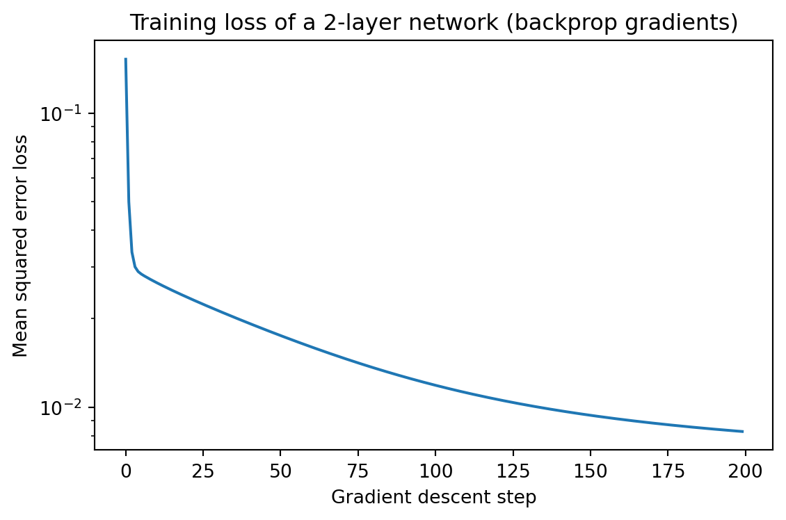
The cell below implements the full forward and backward pass for a small two-layer network in vectorized form, verifies the analytic gradients against a numerical finite-difference gradient, and trains the network with gradient descent. The same three equations derived above, the output error, the propagation recurrence, and the outer-product parameter gradient, drive the entire computation.
Gradient check W1: max relative error = 1.02e-10
Gradient check W2: max relative error = 4.80e-11
Initial loss: 0.1523
Final loss:   0.0083
The relative errors print as roughly \(10^{-10}\), confirming the analytic backpropagation gradients match the numerical reference to machine precision, and the loss curve falls by more than an order of magnitude as gradient descent consumes those gradients.
A central and somewhat surprising result is that the backward pass costs only a small constant factor more than the forward pass. For a feedforward network the dominant operation in each layer is the matrix-vector product \(W^{(\ell)} \mathbf{a}^{(\ell-1)}\). If layer \(\ell\) has \(n_\ell\) units, this product costs on the order of \(n_\ell \, n_{\ell-1}\) multiply-add operations. The forward pass cost is therefore \(\sum_\ell n_\ell n_{\ell-1}\).
In the backward pass each layer performs two operations of the same shape: the propagation \(\big(W^{(\ell)}\big)^\top \boldsymbol{\delta}^{(\ell)}\) and the outer product \(\boldsymbol{\delta}^{(\ell)} \big(\mathbf{a}^{(\ell-1)}\big)^\top\). Each is again on the order of \(n_\ell n_{\ell-1}\) operations. The backward pass thus costs roughly twice the forward pass, and the combined forward-plus-backward cost is about three times a single forward evaluation. The cheap-gradient result generalizes: for any function computed by a program, reverse-mode autodiff produces the full gradient at a cost that is a constant multiple, typically in the range of two to four, of the cost of evaluating the function. This constant is independent of the number of parameters, which is what makes training networks with billions of parameters feasible.
28.5.2 5.2 Memory cost
The time efficiency of reverse mode is bought with memory. The backward recurrence for \(\boldsymbol{\delta}^{(\ell)}\) requires \(\mathbf{z}^{(\ell)}\) and \(\mathbf{a}^{(\ell-1)}\), quantities computed during the forward pass. The engine must therefore retain the intermediate activations of every layer until the backward pass consumes them. Memory consumption scales with the depth of the network times the size of the activations, which for large models and large batch sizes becomes the binding constraint on what can be trained on a given device. Forward mode, by contrast, needs only constant extra memory beyond the function evaluation, since it carries tangents alongside values and discards them as it advances.
28.5.3 5.3 Gradient checkpointing and the time-memory trade
Because activation memory often dominates, a standard technique trades time for memory. Gradient checkpointing stores only a subset of activations, the checkpoints, during the forward pass and discards the rest. During the backward pass the discarded activations are recomputed on demand by re-running short segments of the forward pass from the nearest checkpoint. With checkpoints placed every \(\sqrt{L}\) layers, memory drops from order \(L\) to order \(\sqrt{L}\) at the cost of roughly one extra forward pass. This trade is what allows very deep networks and long-context transformers to fit in limited device memory, and it is a direct practical consequence of the asymmetric memory profile of reverse mode.
28.5.4 5.4 Batching and parallelism
In practice the activation vectors \(\mathbf{a}^{(\ell)}\) become matrices whose columns are the examples in a minibatch, and the matrix-vector products become matrix-matrix products. This raises arithmetic intensity, the ratio of compute to memory traffic, which is exactly what modern accelerators reward. The chain-rule structure is unchanged; the error \(\boldsymbol{\delta}^{(\ell)}\) simply gains a batch dimension, and the weight gradient becomes a sum of outer products over the batch, expressed as a single matrix multiplication \(\boldsymbol{\delta}^{(\ell)} \big(A^{(\ell-1)}\big)^\top\). The backward pass over a batch is therefore as parallelizable as the forward pass, and the whole training step maps cleanly onto GPU and TPU hardware. This alignment between the mathematics of the chain rule and the strengths of parallel hardware is a large part of why the backpropagation-plus-gradient-descent recipe has scaled so far.
28.5.5 5.5 Numerical considerations
Two numerical issues deserve mention. First, the repeated multiplication of chain-rule factors in deep networks can drive gradients toward zero or infinity, the vanishing and exploding gradient problems noted in Section 1.1. Architectural choices such as residual connections, careful initialization, and normalization layers exist largely to keep the product of backward factors near unit scale so that gradients neither collapse nor blow up across many layers. Second, autodiff computes exact derivatives up to floating-point rounding, which makes it far more accurate than finite-difference approximations and free of the step-size dilemma that plagues numerical differentiation. The combination of exactness, low constant-factor cost, and hardware alignment is what makes reverse-mode automatic differentiation the foundation on which essentially all of modern deep learning is built.
28.6 References
Rumelhart, D. E., Hinton, G. E., and Williams, R. J. (1986). Learning representations by back-propagating errors. Nature, 323, 533-536. DOI: 10.1038/323533a0
Baydin, A. G., Pearlmutter, B. A., Radul, A. A., and Siskind, J. M. (2018). Automatic Differentiation in Machine Learning: a Survey. Journal of Machine Learning Research, 18(153), 1-43. https://jmlr.org/papers/v18/17-468.html
Linnainmaa, S. (1976). Taylor expansion of the accumulated rounding error. BIT Numerical Mathematics, 16(2), 146-160. DOI: 10.1007/BF01931367
Werbos, P. J. (1990). Backpropagation through time: what it does and how to do it. Proceedings of the IEEE, 78(10), 1550-1560. DOI: 10.1109/5.58337
Goodfellow, I., Bengio, Y., and Courville, A. (2016). Deep Learning, Chapter 6: Deep Feedforward Networks. MIT Press. https://www.deeplearningbook.org/contents/mlp.html
Griewank, A., and Walther, A. (2008). Evaluating Derivatives: Principles and Techniques of Algorithmic Differentiation, 2nd edition. SIAM. DOI: 10.1137/1.9780898717761
Nielsen, M. (2015). Neural Networks and Deep Learning, Chapter 2: How the backpropagation algorithm works. http://neuralnetworksanddeeplearning.com/chap2.html
Chen, T., Xu, B., Zhang, C., and Guestrin, C. (2016). Training Deep Nets with Sublinear Memory Cost. arXiv:1604.06174. DOI: 10.48550/arXiv.1604.06174
Paszke, A., Gross, S., Massa, F., et al. (2019). PyTorch: An Imperative Style, High-Performance Deep Learning Library. Advances in Neural Information Processing Systems 32, 8024-8035. DOI: 10.48550/arXiv.1912.01703
Source Code
# The Chain Rule and BackpropagationBackpropagation is the computational engine of modern deep learning. Every time a neural network learns, it adjusts its parameters in a direction that reduces a loss, and the gradient that defines that direction is computed by backpropagation. At its mathematical core, backpropagation is nothing more than a disciplined application of the chain rule from calculus, organized so that the gradient of a scalar loss with respect to millions or billions of parameters can be computed in a single sweep that costs about the same as evaluating the network itself. This chapter builds the idea from the ground up. We begin with the chain rule in one and several variables, formalize the notion of a computational graph, contrast forward-mode and reverse-mode automatic differentiation, derive backpropagation for a feedforward network in full, and then account precisely for its computational cost.## 1. The Chain Rule### 1.1 The single-variable chain ruleSuppose $y = f(u)$ and $u = g(x)$, so that $y$ depends on $x$ through the intermediate quantity $u$. The composition is $y = f(g(x))$, and the single-variable chain rule states$$\frac{dy}{dx} = \frac{dy}{du} \cdot \frac{du}{dx} = f'(g(x)) \, g'(x).$$The rule says that the sensitivity of the output to the input is the product of the local sensitivities along the path of dependence. If a small change $\Delta x$ produces a change $\Delta u \approx g'(x)\,\Delta x$, and that change in turn produces $\Delta y \approx f'(u)\,\Delta u$, then composing gives $\Delta y \approx f'(u)\,g'(x)\,\Delta x$. This multiplicative structure is the seed of everything that follows. Backpropagation is the systematic propagation of such local sensitivities backward through a chain of operations.A longer chain composes more factors. If $y = f_n(f_{n-1}(\cdots f_1(x)\cdots))$, write $u_0 = x$ and $u_k = f_k(u_{k-1})$. Then$$\frac{dy}{dx} = \prod_{k=1}^{n} \frac{du_k}{du_{k-1}} = f_n'(u_{n-1}) \, f_{n-1}'(u_{n-2}) \cdots f_1'(u_0).$$A deep network is exactly such a deep composition, with each layer playing the role of one $f_k$. The product form already hints at a practical concern: when many factors are smaller than one in magnitude the product shrinks toward zero, and when many exceed one it explodes. These are the vanishing and exploding gradient phenomena, and they are direct consequences of multiplying many chain-rule factors.### 1.2 The multivariable chain ruleNeural networks operate on vectors and matrices, so we need the chain rule for functions of several variables. Let $y$ be a scalar that depends on intermediate variables $u_1, \ldots, u_m$, each of which depends on $x$. Then the total derivative accumulates contributions along every path:$$\frac{dy}{dx} = \sum_{j=1}^{m} \frac{\partial y}{\partial u_j} \cdot \frac{\partial u_j}{\partial x}.$$The single-variable rule multiplies; the multivariable rule multiplies and then sums over all intermediate variables through which influence flows. This sum-over-paths structure is what makes a node with several outgoing edges accumulate gradient from each of them.The general vector form is cleaner. Let $\mathbf{f} : \mathbb{R}^n \to \mathbb{R}^m$ and $\mathbf{g} : \mathbb{R}^m \to \mathbb{R}^p$, and consider the composition $\mathbf{h} = \mathbf{g} \circ \mathbf{f}$. The Jacobian of $\mathbf{f}$ at $\mathbf{x}$ is the $m \times n$ matrix $J_{\mathbf{f}}$ with entries $(J_{\mathbf{f}})_{ij} = \partial f_i / \partial x_j$. The chain rule becomes a matrix product:$$J_{\mathbf{h}}(\mathbf{x}) = J_{\mathbf{g}}\big(\mathbf{f}(\mathbf{x})\big) \, J_{\mathbf{f}}(\mathbf{x}),$$a $p \times n$ matrix equal to the product of a $p \times m$ matrix and an $m \times n$ matrix. The order matters because matrix multiplication does not commute, and the dimensions must chain through the shared size $m$. The entire theory of automatic differentiation is a study of how to evaluate such chained Jacobian products efficiently, and in particular how to avoid ever forming the full Jacobians when we only need a single row or a single column of the final result.### 1.3 Gradients, Jacobians, and the scalar-output special caseIn supervised learning the loss $L$ is a scalar. When the final output is a scalar, the Jacobian $J_{\mathbf{h}}$ has a single row, and that row is the gradient $\nabla L$ transposed. This asymmetry, a scalar output and a high-dimensional input, is precisely the regime in which one direction of evaluating the Jacobian product is dramatically cheaper than the other. Holding this fact in mind motivates the choice of reverse-mode differentiation, which we develop after introducing computational graphs.It helps to fix two pieces of notation. For a scalar-valued function $L$ of a vector $\mathbf{z}$, the gradient $\nabla_{\mathbf{z}} L$ is the vector of partial derivatives $\partial L / \partial z_i$. We will write $\bar{\mathbf{z}} = \nabla_{\mathbf{z}} L$ and call it the adjoint of $\mathbf{z}$. The adjoint of a variable answers the question: if I perturb this variable slightly, how much does the final loss change? Backpropagation is an algorithm for computing the adjoint of every variable in the graph.## 2. Computational Graphs### 2.1 Representing a computation as a graphA computational graph is a directed acyclic graph in which each node represents a variable produced by an elementary operation, and each edge represents a data dependency. Leaf nodes with no incoming edges are inputs and parameters. Interior nodes are intermediate results. A designated output node holds the final value, the scalar loss in our setting.Consider the small expression $L = (wx + b - y)^2$, a single linear unit followed by a squared error against a target $y$. Decomposing into elementary operations gives$$p = w x, \qquad q = p + b, \qquad r = q - y, \qquad L = r^2.$$As a graph:``` w ---\ (*) --> p ---\ x ---/ (+) --> q ---\ b ----/ (-) --> r --> (square) --> L y ------/```Each interior node knows how to compute its value from its inputs (the forward operation) and how to compute the local partial derivative of its output with respect to each input. For the multiply node $p = wx$, the local partials are $\partial p / \partial w = x$ and $\partial p / \partial x = w$. For the square node $L = r^2$, the local partial is $\partial L / \partial r = 2r$. These local rules are fixed and known in advance for each operation type. The global derivative emerges from composing them along the graph.### 2.2 The forward passEvaluating the graph means visiting the nodes in topological order, so that every node is computed only after all of its inputs are available, and recording each intermediate value. For concrete numbers $w = 2$, $x = 3$, $b = 1$, $y = 4$, the forward pass yields $p = 6$, $q = 7$, $r = 3$, and $L = 9$. The stored intermediate values are not waste; they are exactly the quantities the backward pass will need, because local derivatives such as $\partial p / \partial w = x$ and $\partial L / \partial r = 2r$ depend on the values computed during the forward pass. The trade of memory for the ability to differentiate is fundamental, and it is why training a network has a larger memory footprint than running it for inference.### 2.3 Why a graph and not a formulaOne could in principle write $L$ as a single closed-form expression in $w, x, b, y$ and differentiate symbolically. For a deep network this is hopeless: the symbolic expression for the gradient grows explosively because shared subexpressions are duplicated every time the product rule or chain rule is applied. The graph representation keeps shared subexpressions shared. Each node is computed once, its adjoint is computed once, and intermediate results are reused rather than re-expanded. This reuse is the difference between an algorithm that scales to billions of parameters and one that does not.## 3. Automatic Differentiation: Forward and Reverse ModeAutomatic differentiation, abbreviated autodiff, computes exact derivatives of functions expressed as programs. It is neither numerical differentiation by finite differences, which is approximate and noisy, nor symbolic differentiation, which produces unwieldy expressions. Autodiff evaluates derivatives to machine precision by applying the chain rule to the elementary operations of the program, reusing the computational graph. There are two principal modes, distinguished by the direction in which derivatives propagate.### 3.1 Forward-mode differentiationForward-mode autodiff propagates derivatives in the same direction as the forward computation, from inputs toward outputs. Alongside each variable $v$ we carry a tangent $\dot{v} = \partial v / \partial x$, the derivative of $v$ with respect to one chosen input $x$. We seed the input we differentiate with respect to by setting its tangent to one and all other input tangents to zero, then propagate.For each operation we apply the chain rule forward. With $p = wx$ and we are differentiating with respect to $w$, the tangent is $\dot{p} = \dot{w} x + w \dot{x}$. Seeding $\dot{w} = 1$ and $\dot{x} = 0$, we get $\dot{p} = x$. Carrying tangents through the whole graph yields $\partial L / \partial w$ at the output. A single forward-mode sweep computes the derivative of all outputs with respect to one input. Equivalently, it computes one column of the Jacobian, namely the Jacobian-vector product $J \mathbf{v}$ for the seed vector $\mathbf{v}$.Forward mode is efficient when the number of inputs is small relative to the number of outputs. To obtain the full gradient of a function with $n$ inputs you must run $n$ separate forward sweeps, one per input. For a neural network with millions of parameters as inputs and a single scalar loss as output, this is catastrophically expensive.### 3.2 Reverse-mode differentiationReverse-mode autodiff propagates derivatives in the opposite direction, from the output back toward the inputs. It computes adjoints $\bar{v} = \partial L / \partial v$, the sensitivity of the final scalar output to each variable. We seed the output with $\bar{L} = \partial L / \partial L = 1$ and then sweep backward through the graph in reverse topological order.The propagation rule is the multivariable chain rule applied locally. If a variable $v$ feeds into operations producing children $c_1, \ldots, c_k$, then by summing over all paths,$$\bar{v} = \sum_{i=1}^{k} \bar{c_i} \, \frac{\partial c_i}{\partial v}.$$Each child contributes its own adjoint times the local partial derivative of that child with respect to $v$, and the contributions add. A single reverse sweep computes the derivative of one output with respect to all inputs. Equivalently it computes one row of the Jacobian, the vector-Jacobian product $\mathbf{u}^\top J$ for the seed $\mathbf{u}$.Reverse mode is efficient when the number of outputs is small relative to the number of inputs. For a scalar loss and many parameters, a single reverse sweep delivers the entire gradient. This is exactly the neural network training regime, and reverse-mode autodiff applied to a neural network is what we call backpropagation.### 3.3 Choosing a mode: the cost asymmetryLet $f : \mathbb{R}^n \to \mathbb{R}^m$. Computing the full $m \times n$ Jacobian by forward mode costs $n$ sweeps, one per input column. By reverse mode it costs $m$ sweeps, one per output row. The cost of each sweep is a small constant multiple of the cost of evaluating $f$ once. Therefore forward mode wins when $n \ll m$ and reverse mode wins when $m \ll n$.``` forward mode: cost ~ n x cost(f) good when few inputs reverse mode: cost ~ m x cost(f) good when few outputs```Deep learning lives at the extreme $m = 1$ (the scalar loss) and $n$ in the millions or billions. Reverse mode computes the whole gradient in cost proportional to a single function evaluation, independent of $n$. That single fact is why reverse-mode autodiff, and hence backpropagation, dominates the field. The price reverse mode pays is memory: it must store the intermediate values from the forward pass until they are consumed during the backward pass, whereas forward mode can discard intermediates as it goes.### 3.4 A tiny reverse-mode autodiff sketchThe following non-executable sketch shows the essential structure of a reverse-mode engine. Each value records its parents and a local backward closure that knows how to push adjoints to those parents.```pythonclass Value:def__init__(self, data, parents=(), backward=lambda g: ()):self.data = data # forward valueself.grad =0.0# accumulated adjointself.parents = parents # input Valuesself._backward = backward # pushes grad to parentsdef mul(a, b): out = Value(a.data * b.data, parents=(a, b))def backward(g): # g is d L / d out a.grad += g * b.data # local partial wrt a is b b.grad += g * a.data # local partial wrt b is a out._backward = backwardreturn outdef backprop(loss): loss.grad =1.0# seed the output adjointfor node in reverse_topological(loss): node._backward(node.grad) # push adjoints to parents```The two lines inside `mul`'s backward closure are the chain rule. The `+=` is the sum-over-paths rule from the multivariable chain rule: when a value is used in several places, gradient accumulates across all of its uses. Every production framework, from PyTorch to JAX, is an elaboration of this skeleton with efficient tensor operations, in-place memory management, and hardware acceleration.## 4. Backpropagation in a Feedforward NetworkWe now derive backpropagation in full for a multilayer feedforward network. The derivation is purely the reverse-mode chain rule specialized to the layered structure of the network.### 4.1 Forward pass notationConsider a network with $L$ layers. Layer $\ell$ has weight matrix $W^{(\ell)}$ and bias vector $\mathbf{b}^{(\ell)}$. Let $\mathbf{a}^{(0)} = \mathbf{x}$ be the input. For each layer $\ell = 1, \ldots, L$ define the pre-activation and activation:$$\mathbf{z}^{(\ell)} = W^{(\ell)} \mathbf{a}^{(\ell-1)} + \mathbf{b}^{(\ell)}, \qquad \mathbf{a}^{(\ell)} = \sigma\big(\mathbf{z}^{(\ell)}\big),$$where $\sigma$ is an elementwise activation function. The network output is $\hat{\mathbf{y}} = \mathbf{a}^{(L)}$, and the loss is a scalar $L_{\text{loss}} = \mathcal{C}(\hat{\mathbf{y}}, \mathbf{y})$ comparing the prediction to a target $\mathbf{y}$. We write the loss symbol as $\mathcal{C}$ to avoid colliding with the layer count $L$.As a graph the layered structure is a simple chain of blocks:``` x=a0 -> [W1,b1] -> z1 -> sigma -> a1 -> [W2,b2] -> z2 -> sigma -> a2 -> ... -> aL -> C```The forward pass walks left to right, storing every $\mathbf{z}^{(\ell)}$ and $\mathbf{a}^{(\ell)}$. The backward pass walks right to left, computing an adjoint for each stored quantity and for each parameter.### 4.2 The output-layer errorDefine the error of layer $\ell$ as the adjoint of its pre-activation,$$\boldsymbol{\delta}^{(\ell)} = \frac{\partial \mathcal{C}}{\partial \mathbf{z}^{(\ell)}} = \bar{\mathbf{z}}^{(\ell)}.$$This vector is the central object of backpropagation. Everything else follows from it. Start at the output. By the chain rule through the elementwise activation $\mathbf{a}^{(L)} = \sigma(\mathbf{z}^{(L)})$,$$\boldsymbol{\delta}^{(L)} = \frac{\partial \mathcal{C}}{\partial \mathbf{a}^{(L)}} \odot \sigma'\big(\mathbf{z}^{(L)}\big),$$where $\odot$ is the elementwise (Hadamard) product and $\sigma'$ is applied elementwise. The first factor $\partial \mathcal{C} / \partial \mathbf{a}^{(L)} = \nabla_{\hat{\mathbf{y}}} \mathcal{C}$ is the gradient of the loss with respect to the prediction, which depends on the chosen loss function. The second factor is the local derivative of the activation. Their elementwise product is the output error.A convenient simplification arises with matched loss and output activation. For softmax output with cross-entropy loss, or for linear output with squared error, the two factors combine to the clean form $\boldsymbol{\delta}^{(L)} = \hat{\mathbf{y}} - \mathbf{y}$, the raw difference between prediction and target. This is not a coincidence; these pairings are designed so that the output error is exactly the residual.### 4.3 Backpropagating the errorNow propagate the error from layer $\ell + 1$ back to layer $\ell$. The pre-activation $\mathbf{z}^{(\ell)}$ influences the loss only through $\mathbf{a}^{(\ell)} = \sigma(\mathbf{z}^{(\ell)})$, which in turn influences $\mathbf{z}^{(\ell+1)} = W^{(\ell+1)} \mathbf{a}^{(\ell)} + \mathbf{b}^{(\ell+1)}$. Applying the multivariable chain rule across this two-step path,$$\boldsymbol{\delta}^{(\ell)} = \left( \big(W^{(\ell+1)}\big)^\top \boldsymbol{\delta}^{(\ell+1)} \right) \odot \sigma'\big(\mathbf{z}^{(\ell)}\big).$$The transpose of the weight matrix appears because we are now reading the linear map backward. In the forward direction $W^{(\ell+1)}$ maps activations of layer $\ell$ to pre-activations of layer $\ell+1$; in the backward direction the adjoint of that linear map is its transpose, which maps the error of layer $\ell+1$ back to the activation space of layer $\ell$. The Hadamard product with $\sigma'(\mathbf{z}^{(\ell)})$ then passes the error through the activation, exactly mirroring the forward pass but in reverse. This single recurrence, applied from $\ell = L-1$ down to $\ell = 1$, is the heart of backpropagation.### 4.4 Parameter gradientsOnce we have the error $\boldsymbol{\delta}^{(\ell)}$ for every layer, the gradients with respect to the parameters follow immediately. Since $\mathbf{z}^{(\ell)} = W^{(\ell)} \mathbf{a}^{(\ell-1)} + \mathbf{b}^{(\ell)}$, the local partials are $\partial z^{(\ell)}_i / \partial W^{(\ell)}_{ij} = a^{(\ell-1)}_j$ and $\partial z^{(\ell)}_i / \partial b^{(\ell)}_i = 1$. Combining with the error gives$$\frac{\partial \mathcal{C}}{\partial W^{(\ell)}} = \boldsymbol{\delta}^{(\ell)} \big(\mathbf{a}^{(\ell-1)}\big)^\top, \qquad \frac{\partial \mathcal{C}}{\partial \mathbf{b}^{(\ell)}} = \boldsymbol{\delta}^{(\ell)}.$$The weight gradient is an outer product of the layer error and the incoming activation. Intuitively, the gradient for weight $W^{(\ell)}_{ij}$ is large when both the error $\delta^{(\ell)}_i$ at the receiving unit and the activation $a^{(\ell-1)}_j$ at the sending unit are large. The bias gradient is simply the error itself, because a bias couples to its pre-activation with unit sensitivity.### 4.5 The complete algorithmAssembling the pieces gives the backpropagation algorithm in full. Forward pass:``` a0 = x for L = 1 .. L: z[L] = W[L] a[L-1] + b[L] a[L] = sigma(z[L]) yhat = a[L]; C = loss(yhat, y)```Backward pass:``` delta = grad_yhat_C (.) sigma'(z[L]) # output error for L = L .. 1: dW[L] = delta (a[L-1])^T # weight gradient db[L] = delta # bias gradient if L > 1: delta = (W[L]^T delta) (.) sigma'(z[L-1]) # propagate```Every gradient needed for gradient descent is produced in one forward pass and one backward pass. The structure is mechanical and identical across architectures: store the forward intermediates, seed the output adjoint, and sweep backward applying the local chain rule at each operation. Convolutional layers, attention, normalization, and residual connections all plug into the same framework; only the local forward and backward rules of each operation differ.### 4.6 A worked micro-exampleTake a two-layer scalar network with $a_0 = x$, $z_1 = w_1 x + b_1$, $a_1 = \sigma(z_1)$, $z_2 = w_2 a_1 + b_2$, $\hat{y} = z_2$, and squared-error loss $\mathcal{C} = \tfrac{1}{2}(\hat{y} - y)^2$. The output error is $\delta_2 = \hat{y} - y$. The parameter gradients at layer two are $\partial \mathcal{C} / \partial w_2 = \delta_2 \, a_1$ and $\partial \mathcal{C} / \partial b_2 = \delta_2$. Propagating gives $\delta_1 = w_2 \delta_2 \, \sigma'(z_1)$, and then $\partial \mathcal{C} / \partial w_1 = \delta_1 \, x$ and $\partial \mathcal{C} / \partial b_1 = \delta_1$. Notice how $\delta_2$ flows into $\delta_1$ through the factor $w_2$ and the local activation slope $\sigma'(z_1)$, an instance of the backpropagation recurrence with all quantities reduced to scalars. The same numbers would emerge from running the tiny autodiff engine of Section 3.4 over this graph.To make every quantity concrete, fix $w_1 = 0.5$, $b_1 = 0.1$, $w_2 = -1.5$, $b_2 = 0.2$, with input $x = 1.0$ and target $y = 0.0$, and take $\sigma = \tanh$ so that $\sigma'(z) = 1 - \tanh^2(z)$.The forward pass computes, in order,$$z_1 = 0.5 \cdot 1.0 + 0.1 = 0.6, \qquad a_1 = \tanh(0.6) = 0.5370,$$$$z_2 = -1.5 \cdot 0.5370 + 0.2 = -0.6055, \qquad \hat{y} = -0.6055,$$$$\mathcal{C} = \tfrac{1}{2}(-0.6055 - 0)^2 = 0.1833.$$The backward pass seeds $\delta_2 = \hat{y} - y = -0.6055$ and walks back through the graph:$$\frac{\partial \mathcal{C}}{\partial w_2} = \delta_2 \, a_1 = -0.6055 \cdot 0.5370 = -0.3252, \qquad \frac{\partial \mathcal{C}}{\partial b_2} = \delta_2 = -0.6055.$$The error then propagates into the first layer through $w_2$ and the local slope $\sigma'(z_1) = 1 - 0.5370^2 = 0.7117$:$$\delta_1 = w_2 \, \delta_2 \, \sigma'(z_1) = (-1.5)(-0.6055)(0.7117) = 0.6464,$$$$\frac{\partial \mathcal{C}}{\partial w_1} = \delta_1 \, x = 0.6464, \qquad \frac{\partial \mathcal{C}}{\partial b_1} = \delta_1 = 0.6464.$$A finite-difference check confirms these: perturbing $w_1$ by $\pm 10^{-6}$ and recomputing $\mathcal{C}$ gives a central-difference slope that agrees with $0.6464$ to roughly nine digits. The executable cell in the next section performs exactly this kind of check automatically for a small vectorized network.### 4.7 Backpropagation as a runnable programThe cell below implements the full forward and backward pass for a small two-layer network in vectorized form, verifies the analytic gradients against a numerical finite-difference gradient, and trains the network with gradient descent. The same three equations derived above, the output error, the propagation recurrence, and the outer-product parameter gradient, drive the entire computation.::: {.panel-tabset}## Python```{python}import numpy as npimport matplotlib.pyplot as pltrng = np.random.default_rng(0)# Tiny 2-layer network: input (3) -> hidden (4, tanh) -> output (1, linear)N, d_in, d_h, d_out =64, 3, 4, 1X = rng.standard_normal((N, d_in))true_w = rng.standard_normal((d_in, 1))y = X @ true_w +0.1* rng.standard_normal((N, 1))W1 =0.5* rng.standard_normal((d_in, d_h)); b1 = np.zeros((1, d_h))W2 =0.5* rng.standard_normal((d_h, d_out)); b2 = np.zeros((1, d_out))def forward(X, W1, b1, W2, b2): z1 = X @ W1 + b1 # pre-activation, layer 1 a1 = np.tanh(z1) # activation, layer 1 z2 = a1 @ W2 + b2 # pre-activation, layer 2return z1, a1, z2, z2 # linear output: yhat = z2def loss_fn(yhat, y):return0.5* np.mean(np.sum((yhat - y) **2, axis=1))def backward(X, y, W1, b1, W2, b2): z1, a1, z2, yhat = forward(X, W1, b1, W2, b2) N = X.shape[0] delta2 = (yhat - y) / N # output error dW2 = a1.T @ delta2 # outer-product gradient db2 = delta2.sum(axis=0, keepdims=True) delta1 = (delta2 @ W2.T) * (1.0- a1 **2) # propagate, tanh' = 1 - a1^2 dW1 = X.T @ delta1 db1 = delta1.sum(axis=0, keepdims=True)return (dW1, db1, dW2, db2), loss_fn(yhat, y)# Numerical gradient check via central finite differencesdef numerical_grad(P, eps=1e-6): grad = np.zeros_like(P) it = np.nditer(P, flags=["multi_index"])whilenot it.finished: idx = it.multi_index; orig = P[idx] P[idx] = orig + eps; lp = loss_fn(forward(X, W1, b1, W2, b2)[3], y) P[idx] = orig - eps; lm = loss_fn(forward(X, W1, b1, W2, b2)[3], y) P[idx] = orig; grad[idx] = (lp - lm) / (2* eps); it.iternext()return grad(an_dW1, _, an_dW2, _), _ = backward(X, y, W1, b1, W2, b2)rel_W1 = np.max(np.abs(an_dW1 - numerical_grad(W1))) / (np.max(np.abs(an_dW1)) +1e-12)rel_W2 = np.max(np.abs(an_dW2 - numerical_grad(W2))) / (np.max(np.abs(an_dW2)) +1e-12)print(f"Gradient check W1: max relative error = {rel_W1:.2e}")print(f"Gradient check W2: max relative error = {rel_W2:.2e}")# Train with gradient descentlr, losses =0.5, []for step inrange(200): (dW1, db1, dW2, db2), L = backward(X, y, W1, b1, W2, b2) W1 -= lr * dW1; b1 -= lr * db1 W2 -= lr * dW2; b2 -= lr * db2 losses.append(L)print(f"Initial loss: {losses[0]:.4f}")print(f"Final loss: {losses[-1]:.4f}")fig, ax = plt.subplots(figsize=(6, 4))ax.plot(losses, color="C0")ax.set_xlabel("Gradient descent step")ax.set_ylabel("Mean squared error loss")ax.set_title("Training loss of a 2-layer network (backprop gradients)")ax.set_yscale("log")fig.tight_layout()plt.show()```The relative errors print as roughly $10^{-10}$, confirming the analytic backpropagation gradients match the numerical reference to machine precision, and the loss curve falls by more than an order of magnitude as gradient descent consumes those gradients.## Julia```julia# Idiomatic Julia: same 2-layer network, forward + backward by hand.usingRandom, StatisticsRandom.seed!(0)N, d_in, d_h, d_out =64, 3, 4, 1X =randn(N, d_in)true_w =randn(d_in, 1)y = X * true_w .+0.1.*randn(N, 1)W1 =0.5.*randn(d_in, d_h); b1 =zeros(1, d_h)W2 =0.5.*randn(d_h, d_out); b2 =zeros(1, d_out)forward(X, W1, b1, W2, b2) =begin z1 = X * W1 .+ b1 a1 =tanh.(z1) z2 = a1 * W2 .+ b2 (z1, a1, z2, z2) # yhat = z2 (linear output)endloss_fn(yhat, y) =0.5*mean(sum((yhat .- y) .^2, dims =2))functionbackward(X, y, W1, b1, W2, b2) z1, a1, z2, yhat =forward(X, W1, b1, W2, b2) n =size(X, 1) delta2 = (yhat .- y) ./ n # output error dW2 = a1'* delta2 # outer-product gradient db2 =sum(delta2, dims =1) delta1 = (delta2 * W2') .* (1.- a1 .^2) # propagate, tanh' dW1 = X'* delta1 db1 =sum(delta1, dims =1) ((dW1, db1, dW2, db2), loss_fn(yhat, y))endlr =0.5for step in1:200 (dW1, db1, dW2, db2), L =backward(X, y, W1, b1, W2, b2)global W1 -= lr .* dW1; global b1 -= lr .* db1global W2 -= lr .* dW2; global b2 -= lr .* db2end_, finalL =backward(X, y, W1, b1, W2, b2)println("Final loss: ", finalL)```## Rust```rust// Idiomatic Rust sketch of one backprop step using nested Vecs.// Matrices are Vec<Vec<f64>>; helpers omitted for brevity.fn matmul(a:&[Vec<f64>], b:&[Vec<f64>]) -> Vec<Vec<f64>> {let (n, k, m) = (a.len(), b.len(), b[0].len()); let mut out = vec![vec![0.0; m]; n];for i in0..n {for t in0..k {for j in0..m { out[i][j] += a[i][t] * b[t][j]; } } } out}fn tanh_mat(z:&[Vec<f64>]) -> Vec<Vec<f64>> {z.iter().map(|r|r.iter().map(|&v|v.tanh()).collect()).collect()}/// One forward + backward pass; returns (loss, dW2) for layer 2.fn step(x:&[Vec<f64>], y:&[Vec<f64>], w1:&[Vec<f64>], w2:&[Vec<f64>]) -> (f64, Vec<Vec<f64>>) { let z1 =matmul(x, w1); let a1 =tanh_mat(&z1); let yhat =matmul(&a1, w2); // linear output let n =x.len() as f64;// output error delta2 = (yhat - y) / N let delta2: Vec<Vec<f64>>=yhat.iter().zip(y).map(|(yh, yt)|yh.iter().zip(yt).map(|(p, t)| (p - t) / n).collect()).collect(); let loss: f64 =yhat.iter().zip(y).map(|(yh, yt)|yh.iter().zip(yt).map(|(p, t)|0.5* (p - t).powi(2)).sum::<f64>()) .sum::<f64>() / n;// dW2 = a1^T *delta2 (outer-product gradient) let a1_t: Vec<Vec<f64>>= (0..a1[0].len()).map(|j|a1.iter().map(|r| r[j]).collect()).collect(); let dw2 =matmul(&a1_t, &delta2); (loss, dw2)}```:::## 5. Computational Cost### 5.1 The forward and backward cost balanceA central and somewhat surprising result is that the backward pass costs only a small constant factor more than the forward pass. For a feedforward network the dominant operation in each layer is the matrix-vector product $W^{(\ell)} \mathbf{a}^{(\ell-1)}$. If layer $\ell$ has $n_\ell$ units, this product costs on the order of $n_\ell \, n_{\ell-1}$ multiply-add operations. The forward pass cost is therefore $\sum_\ell n_\ell n_{\ell-1}$.In the backward pass each layer performs two operations of the same shape: the propagation $\big(W^{(\ell)}\big)^\top \boldsymbol{\delta}^{(\ell)}$ and the outer product $\boldsymbol{\delta}^{(\ell)} \big(\mathbf{a}^{(\ell-1)}\big)^\top$. Each is again on the order of $n_\ell n_{\ell-1}$ operations. The backward pass thus costs roughly twice the forward pass, and the combined forward-plus-backward cost is about three times a single forward evaluation. The cheap-gradient result generalizes: for any function computed by a program, reverse-mode autodiff produces the full gradient at a cost that is a constant multiple, typically in the range of two to four, of the cost of evaluating the function. This constant is independent of the number of parameters, which is what makes training networks with billions of parameters feasible.### 5.2 Memory costThe time efficiency of reverse mode is bought with memory. The backward recurrence for $\boldsymbol{\delta}^{(\ell)}$ requires $\mathbf{z}^{(\ell)}$ and $\mathbf{a}^{(\ell-1)}$, quantities computed during the forward pass. The engine must therefore retain the intermediate activations of every layer until the backward pass consumes them. Memory consumption scales with the depth of the network times the size of the activations, which for large models and large batch sizes becomes the binding constraint on what can be trained on a given device. Forward mode, by contrast, needs only constant extra memory beyond the function evaluation, since it carries tangents alongside values and discards them as it advances.### 5.3 Gradient checkpointing and the time-memory tradeBecause activation memory often dominates, a standard technique trades time for memory. Gradient checkpointing stores only a subset of activations, the checkpoints, during the forward pass and discards the rest. During the backward pass the discarded activations are recomputed on demand by re-running short segments of the forward pass from the nearest checkpoint. With checkpoints placed every $\sqrt{L}$ layers, memory drops from order $L$ to order $\sqrt{L}$ at the cost of roughly one extra forward pass. This trade is what allows very deep networks and long-context transformers to fit in limited device memory, and it is a direct practical consequence of the asymmetric memory profile of reverse mode.### 5.4 Batching and parallelismIn practice the activation vectors $\mathbf{a}^{(\ell)}$ become matrices whose columns are the examples in a minibatch, and the matrix-vector products become matrix-matrix products. This raises arithmetic intensity, the ratio of compute to memory traffic, which is exactly what modern accelerators reward. The chain-rule structure is unchanged; the error $\boldsymbol{\delta}^{(\ell)}$ simply gains a batch dimension, and the weight gradient becomes a sum of outer products over the batch, expressed as a single matrix multiplication $\boldsymbol{\delta}^{(\ell)} \big(A^{(\ell-1)}\big)^\top$. The backward pass over a batch is therefore as parallelizable as the forward pass, and the whole training step maps cleanly onto GPU and TPU hardware. This alignment between the mathematics of the chain rule and the strengths of parallel hardware is a large part of why the backpropagation-plus-gradient-descent recipe has scaled so far.### 5.5 Numerical considerationsTwo numerical issues deserve mention. First, the repeated multiplication of chain-rule factors in deep networks can drive gradients toward zero or infinity, the vanishing and exploding gradient problems noted in Section 1.1. Architectural choices such as residual connections, careful initialization, and normalization layers exist largely to keep the product of backward factors near unit scale so that gradients neither collapse nor blow up across many layers. Second, autodiff computes exact derivatives up to floating-point rounding, which makes it far more accurate than finite-difference approximations and free of the step-size dilemma that plagues numerical differentiation. The combination of exactness, low constant-factor cost, and hardware alignment is what makes reverse-mode automatic differentiation the foundation on which essentially all of modern deep learning is built.## References1. Rumelhart, D. E., Hinton, G. E., and Williams, R. J. (1986). Learning representations by back-propagating errors. Nature, 323, 533-536. DOI: 10.1038/323533a02. Baydin, A. G., Pearlmutter, B. A., Radul, A. A., and Siskind, J. M. (2018). Automatic Differentiation in Machine Learning: a Survey. Journal of Machine Learning Research, 18(153), 1-43. https://jmlr.org/papers/v18/17-468.html3. Linnainmaa, S. (1976). Taylor expansion of the accumulated rounding error. BIT Numerical Mathematics, 16(2), 146-160. DOI: 10.1007/BF019313674. Werbos, P. J. (1990). Backpropagation through time: what it does and how to do it. Proceedings of the IEEE, 78(10), 1550-1560. DOI: 10.1109/5.583375. Goodfellow, I., Bengio, Y., and Courville, A. (2016). Deep Learning, Chapter 6: Deep Feedforward Networks. MIT Press. https://www.deeplearningbook.org/contents/mlp.html6. Griewank, A., and Walther, A. (2008). Evaluating Derivatives: Principles and Techniques of Algorithmic Differentiation, 2nd edition. SIAM. DOI: 10.1137/1.97808987177617. Nielsen, M. (2015). Neural Networks and Deep Learning, Chapter 2: How the backpropagation algorithm works. http://neuralnetworksanddeeplearning.com/chap2.html8. Chen, T., Xu, B., Zhang, C., and Guestrin, C. (2016). Training Deep Nets with Sublinear Memory Cost. arXiv:1604.06174. DOI: 10.48550/arXiv.1604.061749. Paszke, A., Gross, S., Massa, F., et al. (2019). PyTorch: An Imperative Style, High-Performance Deep Learning Library. Advances in Neural Information Processing Systems 32, 8024-8035. DOI: 10.48550/arXiv.1912.01703