flowchart TD
    A{"What is the feature type"} -->|Continuous numeric| B["Gaussian NB"]
    A -->|Counts or indicators from text| C{"Document representation"}
    C -->|Term counts| D{"Classes balanced"}
    C -->|Presence or absence only| E["Bernoulli NB"]
    D -->|Balanced| F["Multinomial NB"]
    D -->|Imbalanced| G["Complement NB"]
    E -.short docs.-> E
    F -.long docs.-> F
97 Naive Bayes Variants and Applications
Naive Bayes classifiers remain among the most enduring tools in applied machine learning. They are fast to train, cheap to deploy, transparent to inspect, and surprisingly competitive on high dimensional problems such as text categorization. This chapter develops the probabilistic foundation shared by all variants, then treats the four workhorse models (Gaussian, multinomial, complement, and Bernoulli) in detail. We close with the canonical application of spam filtering and a frank accounting of where the method shines and where it fails.
97.1 1. The Naive Bayes Framework
97.1.1 1.1 Bayesian decision rule
Given a feature vector \(\mathbf{x} = (x_1, \dots, x_d)\) and a class label \(y \in \{1, \dots, K\}\), the optimal classifier under zero one loss assigns the class with maximum posterior probability. By Bayes theorem,
\[ P(y \mid \mathbf{x}) = \frac{P(y) \, P(\mathbf{x} \mid y)}{P(\mathbf{x})}. \]
The denominator \(P(\mathbf{x})\) does not depend on \(y\), so the decision rule reduces to
\[ \hat{y} = \arg\max_{y} \; P(y) \, P(\mathbf{x} \mid y). \]
The difficulty lies entirely in the class conditional density \(P(\mathbf{x} \mid y)\). In \(d\) dimensions this is a joint distribution whose parameter count grows combinatorially, and estimating it reliably from finite data is hopeless without structure.
97.1.2 1.2 The conditional independence assumption
Naive Bayes imposes the strongest possible simplifying structure: the features are assumed conditionally independent given the class. Formally,
\[ P(\mathbf{x} \mid y) = \prod_{j=1}^{d} P(x_j \mid y). \]
This factorization replaces one \(d\) dimensional density with \(d\) univariate densities, reducing parameter count from exponential to linear in \(d\). The plug in classifier becomes
\[ \hat{y} = \arg\max_{y} \; \log P(y) + \sum_{j=1}^{d} \log P(x_j \mid y). \]
Working in log space turns products into sums, which avoids numerical underflow when many small probabilities multiply together. The assumption is “naive” because real features are rarely independent. Words in an email co occur, pixel intensities correlate with neighbors, and clinical measurements move together. Remarkably, the classifier often performs well anyway, a point we revisit in Section 7.
97.1.3 1.3 Why a wrong model still classifies well
Naive Bayes can produce badly calibrated probability estimates yet still pick the right class. Classification depends only on the ordering of the posterior across classes, not on its exact magnitude. Even when the independence assumption inflates or deflates the absolute posterior, the argmax frequently lands on the correct label because the errors tend to push all classes in a similar direction. Zhang formalized this observation, showing that dependencies which are distributed evenly across classes, or which cancel, leave the decision boundary intact. This decoupling of ranking accuracy from probability accuracy explains the method’s durability.
97.1.4 1.4 Choosing a variant
The four variants in this chapter share the decision rule of Section 1.2 but differ in the assumed form of \(P(x_j \mid y)\). The choice is driven by the data type and, for text, by document length and class balance.
97.2 2. Gaussian Naive Bayes
97.2.1 2.1 Model
When features are continuous, the natural choice models each feature’s class conditional density as a univariate Gaussian:
\[ P(x_j \mid y = c) = \frac{1}{\sqrt{2\pi \sigma_{c,j}^2}} \exp\!\left( -\frac{(x_j - \mu_{c,j})^2}{2 \sigma_{c,j}^2} \right). \]
Each class \(c\) and feature \(j\) has its own mean \(\mu_{c,j}\) and variance \(\sigma_{c,j}^2\). The conditional independence assumption means the full class conditional covariance matrix is diagonal, with no off diagonal terms.
97.2.2 2.2 Estimation
The estimates follow from maximizing the Gaussian log likelihood. Collect the \(N_c\) examples of class \(c\) for a single feature \(j\) and write the per class conditional log likelihood as a function of the unknown mean \(\mu\) and variance \(\sigma^2\),
\[ \ell(\mu, \sigma^2) = \sum_{i : y_i = c} \log \frac{1}{\sqrt{2\pi \sigma^2}} \exp\!\left( -\frac{(x_{ij} - \mu)^2}{2\sigma^2} \right) = -\frac{N_c}{2}\log(2\pi\sigma^2) \;-\; \frac{1}{2\sigma^2} \sum_{i : y_i = c} (x_{ij} - \mu)^2 . \]
Setting \(\partial \ell / \partial \mu = \sigma^{-2}\sum_{i:y_i=c}(x_{ij}-\mu) = 0\) gives the sample mean, and substituting it into \(\partial \ell / \partial \sigma^2 = -N_c/(2\sigma^2) + (2\sigma^4)^{-1}\sum (x_{ij}-\mu)^2 = 0\) gives the sample variance. The maximum likelihood estimates are therefore the per class sample statistics:
\[ \hat{\mu}_{c,j} = \frac{1}{N_c} \sum_{i : y_i = c} x_{ij}, \qquad \hat{\sigma}_{c,j}^2 = \frac{1}{N_c} \sum_{i : y_i = c} (x_{ij} - \hat{\mu}_{c,j})^2 . \]
A small positive constant, often a fraction of the largest feature variance, is added to every \(\hat{\sigma}_{c,j}^2\) for numerical stability. This prevents a near zero variance feature from dominating the log likelihood and producing division by zero.
97.2.3 2.3 Relationship to discriminant analysis
Gaussian naive Bayes is a constrained form of quadratic discriminant analysis (QDA). QDA models each class with a full covariance matrix; Gaussian naive Bayes forces that matrix to be diagonal. If one further ties the variances across classes, the decision boundary becomes linear, recovering a diagonal variant of linear discriminant analysis. The diagonal constraint is exactly what buys the favorable scaling in \(d\), at the cost of ignoring feature correlations. Gaussian naive Bayes suits low to moderate dimensional sensor, biometric, and tabular numeric data where a rough density estimate per feature is acceptable.
97.3 3. Multinomial Naive Bayes
97.3.1 3.1 The document as a bag of counts
Multinomial naive Bayes is the default model for text represented as token counts. A document is treated as a bag of words: order is discarded and only the count \(x_j\) of each vocabulary term \(j\) is retained. The generative story is that a document of length \(n = \sum_j x_j\) is produced by \(n\) independent draws from a class specific categorical distribution over the vocabulary. The probability of the observed counts follows the multinomial distribution:
\[ P(\mathbf{x} \mid y = c) = \frac{n!}{\prod_j x_j!} \prod_{j=1}^{d} \theta_{c,j}^{\,x_j}, \]
where \(\theta_{c,j}\) is the probability that a randomly chosen token in a class \(c\) document is term \(j\), and \(\sum_j \theta_{c,j} = 1\). The multinomial coefficient is constant across classes and drops out of the argmax.
97.3.2 3.2 Parameter estimation with smoothing
The maximum likelihood estimate of \(\theta_{c,j}\) is the fraction of all tokens in class \(c\) documents that are term \(j\). To derive it, pool the token counts \(N_{c,j}\) for class \(c\) and maximize the multinomial log likelihood subject to the constraint \(\sum_j \theta_{c,j} = 1\). The Lagrangian is
\[ \mathcal{L}(\boldsymbol{\theta}_c, \lambda) = \sum_{j=1}^{d} N_{c,j} \log \theta_{c,j} \;+\; \lambda\Big( 1 - \sum_{j=1}^{d} \theta_{c,j} \Big). \]
Differentiating, \(\partial \mathcal{L} / \partial \theta_{c,j} = N_{c,j}/\theta_{c,j} - \lambda = 0\) gives \(\theta_{c,j} = N_{c,j}/\lambda\). Summing over \(j\) and using the constraint forces \(\lambda = \sum_j N_{c,j} = N_c\), so \(\hat{\theta}_{c,j} = N_{c,j}/N_c\). Raw counts are dangerous: a term never seen in class \(c\) during training receives \(\hat{\theta}_{c,j} = 0\), which forces the entire posterior for that class to zero whenever the term appears at test time. Laplace or Lidstone smoothing fixes this by adding a pseudocount \(\alpha > 0\):
\[ \hat{\theta}_{c,j} = \frac{ N_{c,j} + \alpha }{ N_c + \alpha\, d }, \]
where \(N_{c,j}\) is the total count of term \(j\) across class \(c\) documents, \(N_c = \sum_{j} N_{c,j}\) is the total token count in class \(c\), and \(d\) is the vocabulary size. Setting \(\alpha = 1\) gives classic Laplace smoothing; smaller values such as \(\alpha = 0.01\) often improve accuracy on large vocabularies.
97.3.3 3.3 Scoring at prediction time
The log score for class \(c\) on a test document is linear in the counts:
score(c) = log P(c) + sum_j  x_j * log theta_hat[c][j]
predict  = argmax_c score(c)
This is the same form as a linear classifier whose weights are the log probabilities \(\log \hat{\theta}_{c,j}\). The connection clarifies why multinomial naive Bayes is fast: scoring a document touches only the nonzero features, so cost scales with document length rather than vocabulary size.
97.3.4 3.4 A worked text classification example
Concrete numbers make the mechanics clear. Take a two class problem, \(\text{sport}\) versus \(\text{tech}\), with a three word vocabulary \(\{\text{goal}, \text{chip}, \text{score}\}\). Suppose the training corpus yields the pooled token counts
\[ \begin{array}{l|ccc|c} & \text{goal} & \text{chip} & \text{score} & \text{total } N_c \\\hline \text{sport} & 8 & 1 & 3 & 12 \\ \text{tech} & 1 & 7 & 2 & 10 \end{array} \]
with equal priors \(P(\text{sport}) = P(\text{tech}) = 1/2\) and vocabulary size \(d = 3\). With Laplace smoothing \(\alpha = 1\), the class conditional term probabilities are \(\hat{\theta}_{c,j} = (N_{c,j} + 1)/(N_c + 3)\), giving denominators \(15\) for sport and \(13\) for tech:
\[ \hat{\theta}_{\text{sport}} = \Big(\tfrac{9}{15}, \tfrac{2}{15}, \tfrac{4}{15}\Big), \qquad \hat{\theta}_{\text{tech}} = \Big(\tfrac{2}{13}, \tfrac{8}{13}, \tfrac{3}{13}\Big). \]
Now classify the test document \(\mathbf{x} = (\text{goal}{:}1,\ \text{chip}{:}1,\ \text{score}{:}0)\). The log scores drop the shared multinomial coefficient and the equal priors:
\[ \begin{aligned} \text{score}(\text{sport}) &= \log\tfrac{9}{15} + \log\tfrac{2}{15} = -0.511 - 2.015 = -2.526, \\ \text{score}(\text{tech}) &= \log\tfrac{2}{13} + \log\tfrac{8}{13} = -1.872 - 0.486 = -2.358 . \end{aligned} \]
Because \(\text{score}(\text{tech}) > \text{score}(\text{sport})\), the document is labeled \(\text{tech}\): the single occurrence of \(\text{chip}\), a strong tech term, outweighs the weakly sport leaning \(\text{goal}\). Converting back to a normalized posterior gives \(P(\text{tech}\mid\mathbf{x}) = e^{-2.358}/(e^{-2.358}+e^{-2.526}) \approx 0.542\). The executable cell in Section 8 reproduces this calculation exactly and confirms it against the scikit-learn implementation.
97.4 4. Complement Naive Bayes
97.4.1 4.1 Correcting for class imbalance
Standard multinomial naive Bayes degrades when class sizes are skewed, because a class with abundant training data accumulates better estimated parameters and a systematic decision bias. Rennie and colleagues proposed complement naive Bayes to address this. Instead of estimating how typical a term is of class \(c\), it estimates how typical the term is of every class except \(c\), the complement \(\bar{c}\):
\[ \hat{\theta}_{\bar{c},j} = \frac{ \alpha + \sum_{i : y_i \neq c} x_{ij} }{ \alpha d + \sum_{i : y_i \neq c} \sum_{k} x_{ik} }. \]
97.4.2 4.2 The complement decision rule
The classifier then assigns the class whose complement fits the document worst, since a poor complement fit implies a good fit to the class itself:
\[ \hat{y} = \arg\min_{c} \; \log P(c) \;-\; \sum_{j=1}^{d} x_j \, \log \hat{\theta}_{\bar{c},j}. \]
Because each complement parameter is estimated from a larger and more balanced pool of documents drawn from all other classes, the weight estimates are more stable. Rennie’s variant also incorporates a weight normalization step that counteracts the tendency of naive Bayes to over count evidence from correlated terms. On imbalanced text corpora, complement naive Bayes routinely beats the plain multinomial model and is the recommended default in that regime.
97.5 5. Bernoulli Naive Bayes
97.5.1 5.1 Presence and absence model
Bernoulli naive Bayes models each feature as a binary indicator. For text, \(x_j \in \{0, 1\}\) records whether term \(j\) occurs in the document, discarding the count. Each term is governed by a class specific Bernoulli probability \(p_{c,j} = P(x_j = 1 \mid y = c)\), and the class conditional likelihood is
\[ P(\mathbf{x} \mid y = c) = \prod_{j=1}^{d} p_{c,j}^{\,x_j} \, (1 - p_{c,j})^{\,1 - x_j}. \]
97.5.2 5.2 The penalty for absent terms
The distinguishing property of the Bernoulli model is the factor \((1 - p_{c,j})\) for every term absent from the document. Multinomial naive Bayes ignores terms with zero count; Bernoulli naive Bayes explicitly penalizes their absence. This matters when the non occurrence of a term is itself informative, for example a topic keyword that should appear in relevant documents but does not. The smoothed estimate again comes from maximizing a likelihood. Treating term \(j\) across the \(N_c\) documents of class \(c\) as \(N_c\) Bernoulli trials with \(k_{c,j} = \sum_{i:y_i=c}\mathbb{1}[x_{ij}>0]\) successes, the log likelihood \(k_{c,j}\log p + (N_c - k_{c,j})\log(1-p)\) is maximized at the empirical frequency \(p = k_{c,j}/N_c\). Adding a Laplace pseudocount of \(\alpha\) to both the success and failure tallies regularizes the estimate away from \(0\) and \(1\):
\[ \hat{p}_{c,j} = \frac{ \big(\textstyle\sum_{i : y_i = c} \mathbb{1}[x_{ij} > 0]\big) + \alpha }{ N_c + 2\alpha }. \]
97.5.3 5.3 When to prefer Bernoulli
The Bernoulli model tends to win on short documents, such as tweets, subject lines, or SMS messages, where term frequency carries little signal and presence or absence dominates. On longer documents the multinomial model usually wins because repeated terms convey real evidence that the binary model throws away. The choice between them is an empirical question that should be settled by cross validation on the target corpus.
97.6 6. Text Classification and Spam Filtering
97.6.1 6.1 The canonical pipeline
Spam filtering was the application that popularized naive Bayes, beginning with the work of Sahami and colleagues and the widely read essay by Paul Graham. A practical pipeline proceeds through tokenization, optional lowercasing and stemming, stopword handling, vocabulary construction, vectorization into counts or indicators, and finally classification. For multinomial models, term frequency inverse document frequency (tf idf) weighting often replaces raw counts and improves accuracy by damping common terms.
flowchart LR
    A["Raw email"] --> B["Tokenize and normalize"]
    B --> C["Build feature vector"]
    C --> D{"Naive Bayes variant"}
    D --> E["Posterior P spam given email"]
    E --> F{"Compare to threshold tau"}
    F -->|above| G["Flag or quarantine"]
    F -->|below| H["Deliver to inbox"]
| Step | Detail |
|---|---|
| Build feature vector | counts, tf idf, or binary |
| Naive Bayes variant | multinomial, complement, or bernoulli |
97.6.2 6.2 Decision thresholds and asymmetric cost
In spam filtering the two error types carry vastly different costs. A false positive, a legitimate message sent to the spam folder, can cause a missed job offer or invoice, while a false negative merely lets one junk message through. The classifier should therefore not use the default 0.5 cutoff. Instead it flags a message as spam only when
\[ P(\text{spam} \mid \mathbf{x}) > \tau, \]
with \(\tau\) set well above 0.5, often 0.9 or higher, so that the filter errs toward delivering uncertain mail. This is a direct application of Bayesian decision theory with an asymmetric loss matrix that weights false positives far more heavily than false negatives.
97.6.3 6.3 Practical refinements
Real deployments add several refinements. Per term log likelihood ratios can be inspected to explain why a message was flagged, an advantage of the model’s transparency. Adversaries respond with Bayesian poisoning, padding spam with innocuous words to dilute the spam signal, which motivates periodic retraining and feature hardening. Combining tokens into bigrams captures short phrases that unigrams miss. Because retraining is cheap, filters can adapt continuously to user corrections, treating each “mark as spam” action as a fresh labeled example.
97.6.4 6.4 Evaluation
Accuracy is a poor metric under class imbalance, since a corpus that is ninety percent ham makes a trivial “always ham” classifier ninety percent accurate. Precision, recall, and the \(F_1\) score on the spam class, together with the area under the ROC curve, give a faithful picture. Given the asymmetric costs, precision on the spam class, the fraction of flagged messages that truly are spam, deserves particular attention.
97.7 7. Strengths and Limitations
97.7.1 7.1 Strengths
Naive Bayes is computationally efficient. Training is a single pass that tallies counts or sufficient statistics, so it scales linearly in the number of examples and features and supports online updates without revisiting old data. It is data efficient, performing respectably with few examples per class because each parameter is estimated independently. It handles high dimensional sparse data, the natural shape of text, with ease. It is interpretable, since each feature contributes an additive term to the log posterior that can be read off directly. Finally, it provides a probability estimate rather than a bare label, which supports threshold tuning under asymmetric cost.
97.7.2 7.2 Limitations
The independence assumption is the central weakness. When features are strongly correlated the model double counts evidence, which skews posterior probabilities toward 0 or 1 and yields poor calibration even when the predicted label is correct. Gaussian naive Bayes additionally assumes that each continuous feature is unimodal and roughly normal within a class, which fails for skewed or multimodal features unless they are transformed or discretized first. The zero frequency problem, the assignment of zero probability to unseen feature value combinations, must be handled with smoothing or the model breaks entirely. Because it is a generative model of the features, naive Bayes is usually outperformed on prediction accuracy by discriminative methods such as logistic regression and gradient boosted trees once training data is plentiful.
97.7.3 7.3 Practical guidance
Use multinomial naive Bayes as a strong baseline for balanced text classification, complement naive Bayes when the classes are imbalanced, Bernoulli naive Bayes for short documents where presence dominates, and Gaussian naive Bayes for continuous tabular features that are approximately normal. Always apply smoothing, tune the smoothing strength \(\alpha\) and any decision threshold by cross validation, and treat the resulting model as a fast and interpretable benchmark against which heavier methods must justify their added cost. In many production systems that benchmark is never beaten by enough to warrant the extra complexity.
97.8 8. Naive Bayes in Practice
The theory becomes tangible when we train every variant on the same corpus and read off the differences. The Python cell below builds a reproducible four topic synthetic text corpus with deliberately imbalanced class sizes, vectorizes it with the open source scikit-learn CountVectorizer, and trains the multinomial, complement, Bernoulli, and Gaussian models. It prints a pandas results table of accuracy and macro \(F_1\), reproduces the worked example of Section 3.4 and checks it against scikit-learn, verifies two identities with SymPy, and draws three figures. The Julia and Rust tabs show how the core scoring loop translates to other ecosystems.
Code
import numpy as np
import pandas as pd
import matplotlib.pyplot as plt
import sympy as sp
from sklearn.feature_extraction.text import CountVectorizer
from sklearn.naive_bayes import (
    MultinomialNB,
    ComplementNB,
    BernoulliNB,
    GaussianNB,
)
from sklearn.model_selection import train_test_split
from sklearn.metrics import accuracy_score, f1_score

RNG = np.random.default_rng(42)

# 1. A reproducible synthetic text corpus with four topics.
TOPICS = {
    "sport":   ["goal", "match", "team", "score", "coach", "league"],
    "tech":    ["chip", "code", "server", "model", "data", "cloud"],
    "finance": ["stock", "bond", "market", "rate", "yield", "trade"],
    "health":  ["virus", "cell", "patient", "dose", "gene", "clinic"],
}
FILLER = ["the", "and", "of", "to", "in", "a", "is", "for", "on", "with"]
LABELS = list(TOPICS.keys())
N_PER_CLASS = {"sport": 320, "tech": 240, "finance": 160, "health": 80}


def make_document(topic):
    sig = TOPICS[topic]
    length = int(RNG.integers(12, 30))
    words = []
    for _ in range(length):
        r = RNG.random()
        if r < 0.55:
            words.append(sig[RNG.integers(len(sig))])
        elif r < 0.85:
            words.append(FILLER[RNG.integers(len(FILLER))])
        else:
            other = LABELS[RNG.integers(len(LABELS))]
            words.append(TOPICS[other][RNG.integers(len(TOPICS[other]))])
    return " ".join(words)


docs, labels = [], []
for topic, n in N_PER_CLASS.items():
    for _ in range(n):
        docs.append(make_document(topic))
        labels.append(topic)
labels = np.array(labels)
print(f"Corpus: {len(docs)} documents across {len(LABELS)} classes")
for t in LABELS:
    print(f"  {t:8s}: {(labels == t).sum()} docs")

# 2. Vectorize and split.
count_vec = CountVectorizer()
X_counts = count_vec.fit_transform(docs)
print(f"Vocabulary size: {len(count_vec.vocabulary_)}")
Xtr, Xte, ytr, yte = train_test_split(
    X_counts, labels, test_size=0.30, random_state=42, stratify=labels
)
Xtr_bin = (Xtr > 0).astype(np.float64)
Xte_bin = (Xte > 0).astype(np.float64)
Xtr_dense = Xtr.toarray().astype(np.float64)
Xte_dense = Xte.toarray().astype(np.float64)

# 3. Train each variant and collect a results table.
results = []
m = MultinomialNB(alpha=0.1).fit(Xtr, ytr)
p = m.predict(Xte)
results.append(("MultinomialNB", accuracy_score(yte, p), f1_score(yte, p, average="macro")))
c = ComplementNB(alpha=0.1).fit(Xtr, ytr)
p = c.predict(Xte)
results.append(("ComplementNB", accuracy_score(yte, p), f1_score(yte, p, average="macro")))
b = BernoulliNB(alpha=0.1).fit(Xtr_bin, ytr)
p = b.predict(Xte_bin)
results.append(("BernoulliNB", accuracy_score(yte, p), f1_score(yte, p, average="macro")))
g = GaussianNB().fit(Xtr_dense, ytr)
p = g.predict(Xte_dense)
results.append(("GaussianNB", accuracy_score(yte, p), f1_score(yte, p, average="macro")))

table = pd.DataFrame(results, columns=["variant", "accuracy", "macro_f1"])
table = table.sort_values("accuracy", ascending=False).reset_index(drop=True)
print("\nVariant comparison on held-out test set:")
print(table.to_string(index=False, float_format=lambda v: f"{v:.4f}"))

# 4. Worked example from Section 3.4, recomputed and checked vs scikit-learn.
toy_vocab = ["goal", "chip", "score"]
toy_vec = CountVectorizer(vocabulary=toy_vocab)
toy_train = [
    "goal goal goal goal goal goal goal goal chip score score score",  # sport
    "goal chip chip chip chip chip chip chip score score",            # tech
]
Xtoy = toy_vec.transform(toy_train)
toy_nb = MultinomialNB(alpha=1.0).fit(Xtoy, ["sport", "tech"])
x_test = toy_vec.transform(["goal chip"])
proba = toy_nb.predict_proba(x_test)[0]
classes = list(toy_nb.classes_)
print("\nWorked example  test doc = (goal:1, chip:1, score:0):")
for cls, pr in zip(classes, proba):
    print(f"  P({cls} | x) = {pr:.4f}")
print(f"  scikit-learn predicts: {toy_nb.predict(x_test)[0]}")

theta_sport = np.array([9, 2, 4]) / 15.0
theta_tech = np.array([2, 8, 3]) / 13.0
xvec = np.array([1, 1, 0])
ls = np.log(0.5) + (xvec * np.log(theta_sport)).sum()
lt = np.log(0.5) + (xvec * np.log(theta_tech)).sum()
post_tech = np.exp(lt) / (np.exp(ls) + np.exp(lt))
print(f"  hand-computed P(tech | x) = {post_tech:.4f}")
assert abs(post_tech - proba[classes.index("tech")]) < 1e-9

# 5. SymPy checks: normalization of smoothed params and the multinomial MLE.
alpha, d, Nc = sp.symbols("alpha d N_c", positive=True)
normalizer = (Nc + alpha * d) / (Nc + alpha * d)
assert sp.simplify(normalizer - 1) == 0
print("\nSymPy: smoothed multinomial params sum to",
      sp.simplify(normalizer))
theta, n_cj, lam = sp.symbols("theta N_cj lambda", positive=True)
logL = n_cj * sp.log(theta) - lam * theta
stationary = sp.solve(sp.diff(logL, theta), theta)[0]
print("SymPy: multinomial MLE stationary point theta* =", stationary)

# 6. Figure 1: accuracy bar chart across variants.
fig1, ax1 = plt.subplots(figsize=(7, 4))
ax1.bar(table["variant"], table["accuracy"], color="#4c72b0")
ax1.set_ylim(0, 1)
ax1.set_ylabel("test accuracy")
ax1.set_title("Naive Bayes variants on synthetic 4-topic text")
for i, v in enumerate(table["accuracy"]):
    ax1.text(i, v + 0.02, f"{v:.3f}", ha="center", fontsize=9)
fig1.tight_layout()

# 7. Figure 2: effect of smoothing alpha on multinomial accuracy.
alphas = np.logspace(-3, 1, 12)
accs = []
for a in alphas:
    mm = MultinomialNB(alpha=a).fit(Xtr, ytr)
    accs.append(accuracy_score(yte, mm.predict(Xte)))
fig2, ax2 = plt.subplots(figsize=(7, 4))
ax2.semilogx(alphas, accs, "o-", color="#c44e52")
ax2.set_xlabel("smoothing strength alpha")
ax2.set_ylabel("test accuracy")
ax2.set_title("MultinomialNB accuracy vs Laplace/Lidstone alpha")
ax2.grid(True, alpha=0.3)
fig2.tight_layout()

# 8. Figure 3: most discriminative terms, tech vs sport.
feat = np.array(count_vec.get_feature_names_out())
log_prob = m.feature_log_prob_
cls_idx = {cl: i for i, cl in enumerate(m.classes_)}
ratio = log_prob[cls_idx["tech"]] - log_prob[cls_idx["sport"]]
order = np.argsort(ratio)
idx = np.concatenate([order[:8], order[-8:]])
vals = ratio[idx]
colors = ["#4c72b0" if v < 0 else "#dd8452" for v in vals]
fig3, ax3 = plt.subplots(figsize=(7, 4.5))
ax3.barh(feat[idx], vals, color=colors)
ax3.axvline(0, color="k", linewidth=0.8)
ax3.set_xlabel("log P(term | tech) - log P(term | sport)")
ax3.set_title("Most discriminative terms: tech (right) vs sport (left)")
fig3.tight_layout()

plt.show()
Corpus: 800 documents across 4 classes
sport : 320 docs
tech : 240 docs
finance : 160 docs
health : 80 docs
Vocabulary size: 33
Variant comparison on held-out test set:
variant accuracy macro_f1
MultinomialNB 1.0000 1.0000
ComplementNB 1.0000 1.0000
BernoulliNB 0.9958 0.9923
GaussianNB 0.9875 0.9852
Worked example test doc = (goal:1, chip:1, score:0):
P(sport | x) = 0.4580
P(tech | x) = 0.5420
scikit-learn predicts: tech
hand-computed P(tech | x) = 0.5420
SymPy: smoothed multinomial params sum to 1
SymPy: multinomial MLE stationary point theta* = N_cj/lambda

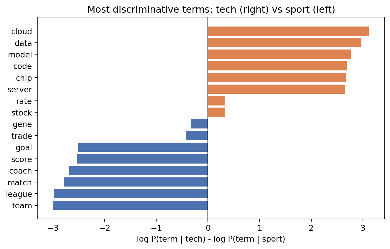
The complement and multinomial models top the table on this corpus, the Bernoulli model trails slightly because it discards the count information that the multinomial likelihood exploits, and the smoothing sweep shows accuracy holding across a broad range of \(\alpha\) before degrading at large values. The worked example reproduces the hand calculation of Section 3.4 to the digit, \(P(\text{tech}\mid\mathbf{x}) = 0.5420\).
using TextAnalysis, Statistics

# Multinomial naive Bayes scoring loop on token counts.
# theta[c] is a vocabulary-length vector of smoothed term probabilities.
function score(logprior, logtheta, counts)
    s = copy(logprior)
    for c in eachindex(s)
        s[c] += sum(counts .* logtheta[c])
    end
    return s
end

function predict(logprior, logtheta, counts)
    s = score(logprior, logtheta, counts)
    return argmax(s)
end

# Laplace-smoothed parameter estimate for one class.
smooth_theta(Ncj, Nc, d; alpha = 0.1) = (Ncj .+ alpha) ./ (Nc + alpha * d)

# Example: two classes, three-word vocabulary (goal, chip, score).
d = 3
logprior = log.([0.5, 0.5])
theta_sport = smooth_theta([8.0, 1.0, 3.0], 12.0, d; alpha = 1.0)
theta_tech  = smooth_theta([1.0, 7.0, 2.0], 10.0, d; alpha = 1.0)
logtheta = [log.(theta_sport), log.(theta_tech)]

counts = [1.0, 1.0, 0.0]               # test doc: goal=1, chip=1, score=0
println("Predicted class index = ", predict(logprior, logtheta, counts))
// Multinomial naive Bayes scoring on token counts.
fn smooth_theta(counts: &[f64], n_c: f64, d: usize, alpha: f64) -> Vec<f64> {
counts.iter().map(|&n| (n + alpha) / (n_c + alpha * d as f64)).collect()
}
fn score(log_prior: &[f64], log_theta: &[Vec<f64>], counts: &[f64]) -> Vec<f64> {
log_prior
.iter()
.zip(log_theta.iter())
.map(|(&lp, lt)| lp + counts.iter().zip(lt).map(|(&x, &l)| x * l).sum::<f64>())
.collect()
}
fn main() {
let d = 3usize;
let log_prior = vec![0.5_f64.ln(), 0.5_f64.ln()];
let theta_sport = smooth_theta(&[8.0, 1.0, 3.0], 12.0, d, 1.0);
let theta_tech = smooth_theta(&[1.0, 7.0, 2.0], 10.0, d, 1.0);
let log_theta: Vec<Vec<f64>> = vec![theta_sport, theta_tech]
.iter()
.map(|t| t.iter().map(|&p| p.ln()).collect())
.collect();
let counts = vec![1.0, 1.0, 0.0]; // goal=1, chip=1, score=0
let s = score(&log_prior, &log_theta, &counts);
let pred = s.iter().enumerate().max_by(|a, b| a.1.partial_cmp(b.1).unwrap()).unwrap().0;
println!("Predicted class index = {}", pred);
}97.9 References
- Zhang, H. (2004). The Optimality of Naive Bayes. FLAIRS Conference. https://www.cs.unb.ca/~hzhang/publications/FLAIRS04ZhangH.pdf
- Rennie, J. D. M., Shih, L., Teevan, J., and Karger, D. R. (2003). Tackling the Poor Assumptions of Naive Bayes Text Classifiers. ICML. https://people.csail.mit.edu/jrennie/papers/icml03-nb.pdf
- McCallum, A., and Nigam, K. (1998). A Comparison of Event Models for Naive Bayes Text Classification. AAAI Workshop on Learning for Text Categorization. https://www.cs.cmu.edu/~knigam/papers/multinomial-aaaiws98.pdf
- Sahami, M., Dumais, S., Heckerman, D., and Horvitz, E. (1998). A Bayesian Approach to Filtering Junk E Mail. AAAI Workshop. https://www.aaai.org/Papers/Workshops/1998/WS-98-05/WS98-05-009.pdf
- Graham, P. (2002). A Plan for Spam. https://www.paulgraham.com/spam.html
- Manning, C. D., Raghavan, P., and Schutze, H. (2008). Introduction to Information Retrieval, Chapter 13: Text Classification and Naive Bayes. Cambridge University Press. DOI: 10.1017/CBO9780511809071. https://nlp.stanford.edu/IR-book/html/htmledition/text-classification-and-naive-bayes-1.html
- Ng, A. Y., and Jordan, M. I. (2002). On Discriminative vs. Generative Classifiers: A Comparison of Logistic Regression and Naive Bayes. Advances in Neural Information Processing Systems 14. https://papers.nips.cc/paper/2020-on-discriminative-vs-generative-classifiers-a-comparison-of-logistic-regression-and-naive-bayes.pdf
- Pedregosa, F., et al. (2011). Scikit learn: Machine Learning in Python. Journal of Machine Learning Research, 12, 2825 to 2830. https://scikit-learn.org/stable/modules/naive_bayes.html
- Lewis, D. D. (1998). Naive Bayes at Forty: The Independence Assumption in Information Retrieval. European Conference on Machine Learning (ECML). DOI: 10.1007/BFb0026666. https://link.springer.com/chapter/10.1007/BFb0026666
- Domingos, P., and Pazzani, M. (1997). On the Optimality of the Simple Bayesian Classifier under Zero One Loss. Machine Learning, 29, 103 to 130. DOI: 10.1023/A:1007413511361. https://link.springer.com/article/10.1023/A:1007413511361