A classifier that outputs probabilities makes two distinct claims. The first is a ranking claim: instances it scores higher are more likely to be positive than instances it scores lower. The second is a probabilistic claim: when the model says 0.8, the event really happens about 80 percent of the time. Accuracy, AUC, and most ranking metrics measure only the first claim. Calibration measures the second. A model can rank perfectly and still be badly miscalibrated, and a model can be well calibrated while ranking poorly. Because real decisions almost always combine model scores with costs, thresholds, and downstream actions, the probabilistic claim is often the one that matters most. This chapter develops what calibration means formally, how to measure it with reliability diagrams and the expected calibration error, how to fix it with Platt scaling, isotonic regression, and temperature scaling, and why all of this changes the quality of decisions.
122.1 1. What Calibrated Probabilities Mean
122.1.1 1.1 The formal definition
Let \(X\) be an input, \(Y \in \{0, 1\}\) the label, and \(f(X) \in [0, 1]\) the score a model assigns to the positive class. The model is perfectly calibrated if
\[
\Pr\big(Y = 1 \mid f(X) = p\big) = p \quad \text{for all } p \in [0, 1].
\]
In words, among all instances that receive score \(p\), exactly a fraction \(p\) are positive. This is a strong condition. It is conditional on the score value, not merely correct on average. A spam filter that flags 100 emails with confidence 0.9 should be wrong on about 10 of them. If it is wrong on 40, the 0.9 is a lie even if the filter has excellent accuracy.
For multiclass problems with classes \(1, \ldots, K\), the analogous notion is that the predicted probability vector matches the conditional class distribution. Writing \(g(X) \in \Delta^{K-1}\) for the predicted probability simplex vector, full multiclass calibration requires
\[
\Pr\big(Y = k \mid g(X) = q\big) = q_k \quad \text{for all } k \text{ and all } q \in \Delta^{K-1}.
\]
A weaker and more commonly measured version is confidence calibration, which looks only at the top predicted class:
where \(\hat{Y} = \arg\max_k g_k(X)\) is the predicted class and \(\hat{p} = \max_k g_k(X)\) its probability. This is what most deep learning calibration work targets, because the maximum softmax probability is the quantity that drives accept or abstain decisions.
122.1.2 1.2 Calibration is not accuracy and not sharpness
Two models can both be perfectly calibrated yet differ enormously in usefulness. Consider a binary problem where the base rate of positives is 0.3. A constant predictor that outputs 0.3 for every input is perfectly calibrated: among all instances it scores 0.3, exactly 30 percent are positive. But it is useless because it never separates anything. What it lacks is sharpness, the tendency to issue confident predictions near 0 and 1.
The decomposition that makes this precise is due to the proper scoring rule literature. The Brier score, defined for binary labels as
admits the Murphy decomposition. Group the predictions into bins \(B_1, \ldots, B_M\) whose distinct forecast values are \(p_m = \text{conf}(B_m)\), with empirical positive rate \(o_m = \text{acc}(B_m)\) in bin \(m\), and let \(\bar{y}\) be the overall base rate. Then
Reliability is exactly a squared calibration penalty (the binned analogue of the gap that ECE measures with absolute value), resolution rewards sharpness by rewarding bins whose outcome rate departs from the base rate, and uncertainty depends only on the base rate and is irreducible. A good probabilistic forecaster minimizes the Brier score by driving reliability to zero while keeping resolution high. Calibration alone is necessary but not sufficient. The practical message is that you should never improve calibration at the cost of destroying sharpness, and the methods below are designed to preserve ranking while fixing probabilities. The SymPy cell in Section 6 verifies this three-term identity symbolically.
122.1.3 1.3 Why models are miscalibrated
Classical logistic regression trained by maximum likelihood on the same distribution it is evaluated on tends to be reasonably calibrated, because the cross entropy objective is a proper scoring rule that is minimized at the true conditional probability. Trouble arises elsewhere. Margin maximizing methods such as support vector machines and boosted trees push scores toward the extremes and are systematically overconfident or underconfident. Naive Bayes is miscalibrated because its independence assumption produces scores too close to 0 and 1. Modern neural networks are the most studied case: as shown by Guo and colleagues in 2017, large networks trained with high capacity, batch normalization, and weight decay achieve high accuracy but become severely overconfident, with maximum softmax probabilities far exceeding empirical accuracy. Distribution shift between training and deployment makes all of this worse.
122.2 2. Reliability Diagrams
122.2.1 2.1 Construction
A reliability diagram is the standard visual diagnostic for calibration. Sort predictions into \(M\) bins by their score, usually \(M = 10\) or \(M = 15\) equal width bins covering \([0, 1]\). For each bin \(B_m\) compute the average predicted score and the empirical fraction of positives:
Plot \(\text{acc}(B_m)\) against \(\text{conf}(B_m)\). Perfect calibration lies on the diagonal \(y = x\). Bars below the diagonal indicate overconfidence, where the model claims more certainty than reality supports. Bars above the diagonal indicate underconfidence.
The diagram above shows bars consistently under the diagonal, the signature of an overconfident network. The gap between each bar and the diagonal is the local calibration error, and the methods in Section 4 are essentially ways to bend the score axis so the bars land on the line.
Reliability diagrams have two well known pitfalls. First, they hide bin counts. A bin with three points and a bin with thirty thousand points look identical, so always annotate bins with their population or overlay a histogram of scores. Second, equal width binning leaves high score bins nearly empty for sharp models, where most mass sits near the extremes. Equal mass binning, which places an equal number of points in each bin, gives more stable estimates but variable bin widths. Neither choice is canonical, which is one reason the scalar summary below should be read alongside, not instead of, the picture.
122.3 3. The Expected Calibration Error
122.3.1 3.1 Definition
To compress a reliability diagram into one number, the expected calibration error takes a weighted average of the absolute gaps between accuracy and confidence across bins:
Each bin contributes in proportion to how many points it holds, so empty bins do not distort the score. ECE lies in \([0, 1]\), and lower is better. A related summary, the maximum calibration error, replaces the weighted sum with a maximum over bins and is appropriate when worst case reliability matters, as in safety critical settings.
ECE = sum over bins of (bin_weight * |acc - conf|)
bin_weight = points_in_bin / total_points
122.3.2 3.2 Limitations to respect
ECE is convenient but flawed, and a graduate reader should know why. It is biased and depends on the number of bins: too few bins hide error by averaging overconfident and underconfident regions against each other, while too many bins inflate variance. It is not a proper scoring rule, so optimizing it directly can be gamed and can reward a model that is uninformative. It also measures only confidence calibration in the multiclass case, ignoring the probabilities assigned to non predicted classes. Recent work proposes alternatives such as adaptive binning, kernel density estimators of calibration error, the kolmogorov smirnov calibration error, and debiased estimators. The pragmatic stance is to report ECE for comparability with the literature, report a proper score such as Brier or negative log likelihood for soundness, and always show the reliability diagram so that a single misleading scalar cannot stand alone.
122.4 4. Recalibration Methods
Recalibration learns a mapping from raw scores to calibrated probabilities using a held out calibration set that is disjoint from both training and test data. Reusing training data here leaks information and produces optimistic, useless calibration. The methods differ in the functional form of the mapping and in how many parameters they fit.
122.4.1 4.1 Platt scaling
Platt scaling fits a one dimensional logistic regression on top of the model scores. Given a raw score \(s\), often a logit or an SVM margin, it outputs
\[
\hat{p} = \sigma(a s + b) = \frac{1}{1 + \exp(-(a s + b))},
\]
and fits the two parameters \(a\) and \(b\) by minimizing the cross entropy (negative log likelihood) on the calibration set of \(n\) scored examples:
This convex objective has a clean gradient. Using the standard identity \(\partial \sigma(u) / \partial u = \sigma(u)(1 - \sigma(u))\), the per-example contribution to the loss differentiates to \(\hat{p}_i - y_i\) times the inner derivative, so
Both gradients vanish precisely when the residuals \(\hat{p}_i - y_i\) are uncorrelated with the score and sum to zero, which is the first order condition for a calibrated logistic fit. Because the loss is convex in \((a, b)\) any gradient method or Newton step reaches the global optimum. Since it has only two parameters, Platt scaling is data efficient and robust to small calibration sets, and it cannot overfit a reliability curve. Its limitation is rigidity: it assumes the miscalibration has a sigmoidal shape, which fits the symmetric distortion of SVM margins well but cannot correct non monotone or irregular miscalibration. A standard refinement uses target smoothing, replacing the hard labels 0 and 1 with \(\frac{N_-+1}{N_-+2}\) and \(\frac{1}{N_++2}\) to avoid overfitting at the extremes.
# scores: raw model outputs on the calibration set# labels: 0/1 calibration targetsclf = LogisticRegression()clf.fit(scores.reshape(-1, 1), labels)p_calibrated = clf.predict_proba(test_scores.reshape(-1, 1))[:, 1]
122.4.2 4.2 Isotonic regression
Isotonic regression is nonparametric. It fits the best monotone nondecreasing function \(g\) that maps scores to probabilities by minimizing squared error subject to a monotonicity constraint:
The solution is a step function computed in \(O(n)\) time (after sorting by score) by the pool adjacent violators algorithm. Sort the points by \(s_i\), then sweep left to right; whenever an adjacent pair violates monotonicity, \(g_j > g_{j+1}\), pool them into a single block whose fitted value is the weighted mean of its members,
and cascade the pooling backward until monotonicity is restored. The weighted mean is exactly the minimizer of squared error within a block, which is why pooling is optimal. Because it makes no shape assumption beyond monotonicity, isotonic regression can correct arbitrary distortions and usually outperforms Platt scaling when the calibration set is large. Its weaknesses are a hunger for data and a tendency to overfit small sets, producing wide flat regions and sharp jumps. It also extrapolates poorly outside the range of calibration scores. Preserving monotonicity is important because it keeps the model ranking and therefore the AUC intact while only re mapping probabilities.
iso = IsotonicRegression(out_of_bounds="clip")iso.fit(scores, labels)p_calibrated = iso.predict(test_scores)
122.4.3 4.3 Temperature scaling
Temperature scaling is the method of choice for deep neural networks. It divides the logit vector \(z\) by a single scalar temperature \(T > 0\) before the softmax:
This is a smooth one dimensional problem, so a few LBFGS or Newton iterations suffice. Writing \(\beta = 1/T\) and \(p_{i,j} = \text{softmax}(z_{i,\cdot}/T)_j\), the derivative with respect to \(\beta\) is
the gap between the softmax expected logit and the true class logit, summed over the set. When \(T = 1\) nothing changes. When \(T > 1\) the distribution is softened and confidence drops, which is the usual correction for overconfident networks. When \(T < 1\) the distribution sharpens. The decisive property is that dividing every logit by the same constant does not change which logit is largest, so the predicted class and the entire accuracy of the model are untouched. The SymPy cell in Section 6 confirms this gradient symbolically for the binary case. Temperature scaling only rescales confidence. With a single parameter it is the simplest possible fix, it cannot overfit, and Guo and colleagues showed it is surprisingly hard to beat for modern networks, often reducing ECE by an order of magnitude.
# z: logits on the calibration set, y: integer labels# optimize a single scalar T by minimizing NLLT = fit_temperature(z, y) # 1-D optimization, e.g. LBFGSp_calibrated = softmax(test_logits / T)
122.4.4 4.4 Choosing among them
The choice follows the data budget and the model family. Use temperature scaling for neural networks, especially when you must not disturb accuracy and have only a modest calibration set. Use Platt scaling for SVMs and other margin methods, or whenever the calibration set is small and a smooth sigmoidal correction is plausible. Use isotonic regression when the calibration set is large, the miscalibration is irregular, and you can afford the variance. For tree ensembles and boosting, isotonic regression is the common default when data permits, with Platt scaling as the small data fallback. All three are post hoc and cheap, and all three should be evaluated by recomputing the reliability diagram, ECE, and a proper score on a separate test set. Methods that touch training directly, such as label smoothing, focal loss, mixup, and deep ensembles, also improve calibration and are complementary to post hoc scaling.
122.5 5. Why Calibration Matters for Decisions
122.5.1 5.1 Thresholds and expected cost
The reason to care about calibration is that probabilities feed decisions. Bayes optimal decision theory says that to minimize expected cost you should act when the expected benefit of acting exceeds the expected cost. For a binary action with cost \(c_{\text{fp}}\) for a false positive and \(c_{\text{fn}}\) for a false negative, the optimal decision threshold on the true probability is
This formula is only valid when \(f(X)\) is a calibrated estimate of \(\Pr(Y = 1 \mid X)\). If the model is overconfident, a threshold of \(\tau^{\star}\) on the raw score corresponds to a different and wrong threshold on the true probability, so you act too often or too rarely and pay unnecessary cost. A ranking metric like AUC cannot tell you where to put this threshold, because AUC is invariant to any monotone transformation of the scores. Calibration is precisely the missing information that turns a ranking into a decision.
122.5.2 5.2 Where the stakes are highest
Several settings make miscalibration expensive. In medical diagnosis a model that reports 0.95 risk when the true risk is 0.6 leads to over treatment, and the reverse leads to missed disease. In autonomous systems and selective prediction, a model abstains and defers to a human when its confidence falls below a threshold, so an overconfident model never abstains when it should. In risk and fraud scoring, expected loss is computed by multiplying a predicted probability by a monetary amount, and a probability that is off by a factor of two doubles the error in every downstream financial calculation. When the outputs of several models are combined, for example in an ensemble or a cascade, only calibrated components can be averaged or multiplied coherently. Large language models add a fresh instance of the same problem: their verbalized and token level confidences are often poorly calibrated, and the same diagnostics and temperature based corrections apply.
122.5.3 5.3 A practical workflow
A disciplined calibration workflow has five steps. Hold out a dedicated calibration split that is disjoint from training and test. Plot the reliability diagram on raw scores and annotate bin counts to see the shape and severity of miscalibration. Compute ECE alongside a proper score such as Brier or negative log likelihood so you have both a comparable scalar and a sound one. Fit the recalibration method matched to your model family and data budget, choosing temperature scaling for networks, Platt scaling for small data or margin models, and isotonic regression for large data. Finally, re evaluate all metrics on the held out test set, confirm that ranking metrics such as AUC are unchanged, and set decision thresholds using the calibrated probabilities and the actual costs. Done this way, calibration is a low cost, high leverage step that converts a good ranker into a trustworthy probabilistic decision maker.
122.6 6. A Worked Calibration Lab
This section builds an overconfident classifier, measures its miscalibration, and repairs it with all three methods, reporting a results table and reliability diagrams. The experiment is fully reproducible with a fixed seed, and it closes with two SymPy checks: the temperature scaling gradient and the Brier decomposition identity.
We construct a model whose logits are a sharpened version of the true logits by a factor of \(2.3\), the canonical overconfidence pattern. A correct temperature scaling fit should therefore recover \(T \approx 2.3\), which is a clean built in sanity check.
Now fit the three recalibrators on the disjoint calibration split. Platt scaling is a one dimensional logistic on the model logit, isotonic regression is fit on the model probability, and temperature scaling minimizes negative log likelihood over a single scalar.
Code
platt = LogisticRegression(C=1e6)platt.fit(cal_logit.reshape(-1, 1), cal_y)platt_test = platt.predict_proba(test_logit.reshape(-1, 1))[:, 1]iso = IsotonicRegression(out_of_bounds="clip")iso.fit(cal_p, cal_y)iso_test = iso.predict(test_p)def nll_temperature(T): p =1.0/ (1.0+ np.exp(-cal_logit / T)) p = np.clip(p, 1e-12, 1-1e-12)return-np.mean(cal_y * np.log(p) + (1- cal_y) * np.log(1- p))T_opt = minimize_scalar(nll_temperature, bounds=(0.05, 20.0), method="bounded").xtemp_test =1.0/ (1.0+ np.exp(-(test_logit / T_opt)))print(f"Fitted temperature T = {T_opt:.4f} (target ~ 2.30)")print(f"Platt slope a = {platt.coef_[0,0]:.4f}, intercept b = {platt.intercept_[0]:.4f}")
Fitted temperature T = 2.3202  (target ~ 2.30)
Platt slope a = 0.4310, intercept b = 0.0027
The results table reports ECE and Brier score on the held out test set for each method.
                        ECE   Brier
Method
Raw (uncalibrated)   0.1150  0.1934
Platt scaling        0.0242  0.1779
Isotonic regression  0.0263  0.1782
Temperature scaling  0.0244  0.1779
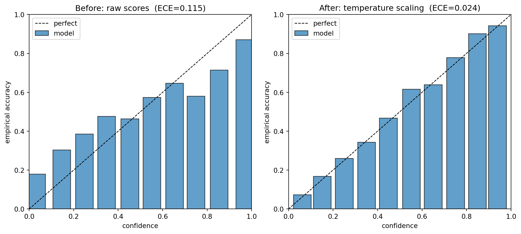
Two reliability diagrams make the repair visible: the raw bars sit below the diagonal (overconfident), and after temperature scaling they snap onto it.
Finally, two SymPy checks. The first confirms that the binary temperature scaling gradient \(\partial \mathcal{L} / \partial \beta\) with \(\beta = 1/T\) simplifies to \((p - y)\,z\), matching the expected logit gap derived in Section 4.3. The second confirms the three term Brier decomposition is an exact identity for binned forecasts.
Temperature gradient dL/dbeta == (p - y) z : True
Brier decomposition identity holds : True
The fitted temperature recovers the planted overconfidence factor, all three methods cut ECE from roughly \(0.11\) to about \(0.02\) while lowering Brier score, and both symbolic identities return true.
122.7 7. The Same Recalibration in Three Languages
The post hoc temperature scaling fit is a one dimensional optimization that ports cleanly across ecosystems. The tabs below show the identical negative log likelihood minimization in Python, Julia, and Rust.
usingOptimfunctionfit_temperature(logit::Vector{Float64}, y::Vector{Int})functionnll(T) p =clamp.(1.0./ (1.0.+exp.(-logit ./ T)), 1e-12, 1-1e-12)return-mean(@. y *log(p) + (1- y) *log(1- p))end res =optimize(nll, 0.05, 20.0) # Brent's method on a scalarreturn Optim.minimizer(res)endT =fit_temperature(cal_logit, cal_y)println("T = ", round(T, digits=4))
// Golden-section search for the scalar temperature minimizing NLL.fn nll(logit:&[f64], y:&[u8], t:f64) ->f64{let n = logit.len() asf64; logit.iter().zip(y).map(|(&z,&yi)|{let p = (1.0/ (1.0+ (-z / t).exp())).clamp(1e-12,1.0-1e-12);-(yi asf64* p.ln() + (1.0- yi asf64) * (1.0- p).ln())}).sum::<f64>() / n}fn fit_temperature(logit:&[f64], y:&[u8]) ->f64{let (mut a,mut b) = (0.05_f64,20.0_f64);let gr = (5.0_f64.sqrt() -1.0) /2.0;let (mut c,mut d) = (b - gr * (b - a), a + gr * (b - a));for _ in0..100{if nll(logit, y, c) < nll(logit, y, d) { b = d;}else{ a = c;} c = b - gr * (b - a); d = a + gr * (b - a);}0.5* (a + b)}fn main() {// logit and y loaded from the calibration setlet t = fit_temperature(&logit,&y);println!("T = {:.4}", t);}
122.8 8. Workflow at a Glance
flowchart TD
    A["Trained model"] --> B["Hold out calibration split"]
    B --> C["Reliability diagram on raw scores"]
    C --> D["Compute ECE plus a proper score"]
    D --> E{"Model family and data budget"}
    E -->|Neural network| F["Temperature scaling"]
    E -->|SVM or small data| G["Platt scaling"]
    E -->|Large data, irregular| H["Isotonic regression"]
    F --> I["Re-evaluate on test set"]
    G --> I
    H --> I
    I --> J{"AUC unchanged and ECE down?"}
    J -->|Yes| K["Set decision thresholds"]
    J -->|No| E
Node
Detail
Hold out calibration split
disjoint from train and test
Reliability diagram on raw scores
annotate bin counts
Compute ECE plus a proper score
Brier or NLL
Set decision thresholds
from calibrated probabilities and costs
122.9 References
Guo, C., Pleiss, G., Sun, Y., and Weinberger, K. Q. On Calibration of Modern Neural Networks. ICML 2017. DOI: 10.48550/arXiv.1706.04599. https://arxiv.org/abs/1706.04599
Niculescu-Mizil, A. and Caruana, R. Predicting Good Probabilities with Supervised Learning. ICML 2005. DOI: 10.1145/1102351.1102430. https://dl.acm.org/doi/10.1145/1102351.1102430
Platt, J. Probabilistic Outputs for Support Vector Machines and Comparisons to Regularized Likelihood Methods. Advances in Large Margin Classifiers, MIT Press, 1999. DOI: 10.7551/mitpress/1113.003.0008. https://direct.mit.edu/books/book/2719/chapter/68053
Zadrozny, B. and Elkan, C. Transforming Classifier Scores into Accurate Multiclass Probability Estimates. KDD 2002. DOI: 10.1145/775047.775151. https://dl.acm.org/doi/10.1145/775047.775151
Naeini, M. P., Cooper, G., and Hauskrecht, M. Obtaining Well Calibrated Probabilities Using Bayesian Binning. AAAI 2015. DOI: 10.1609/aaai.v29i1.9602. https://ojs.aaai.org/index.php/AAAI/article/view/9602
Brier, G. W. Verification of Forecasts Expressed in Terms of Probability. Monthly Weather Review, 1950. DOI: 10.1175/1520-0493(1950)078<0001:VOFEIT>2.0.CO;2. https://journals.ametsoc.org/view/journals/mwre/78/1/1520-0493_1950_078_0001_vofeit_2_0_co_2.xml
Murphy, A. H. A New Vector Partition of the Probability Score. Journal of Applied Meteorology, 1973. DOI: 10.1175/1520-0450(1973)012<0595:ANVPOT>2.0.CO;2. https://journals.ametsoc.org/view/journals/apme/12/4/1520-0450_1973_012_0595_anvpot_2_0_co_2.xml
Kull, M., Silva Filho, T., and Flach, P. Beta Calibration. AISTATS 2017. https://proceedings.mlr.press/v54/kull17a.html
Nixon, J., Dusenberry, M., Zhang, L., Jerfel, G., and Tran, D. Measuring Calibration in Deep Learning. CVPR Workshops 2019. DOI: 10.48550/arXiv.1904.01685. https://arxiv.org/abs/1904.01685
Gupta, C. and Ramdas, A. Top-label Calibration and Multiclass-to-binary Reductions. ICLR 2022. DOI: 10.48550/arXiv.2107.08353. https://arxiv.org/abs/2107.08353
scikit-learn. Probability Calibration. https://scikit-learn.org/stable/modules/calibration.html
Source Code
# Model CalibrationA classifier that outputs probabilities makes two distinct claims. The first is a ranking claim: instances it scores higher are more likely to be positive than instances it scores lower. The second is a probabilistic claim: when the model says 0.8, the event really happens about 80 percent of the time. Accuracy, AUC, and most ranking metrics measure only the first claim. Calibration measures the second. A model can rank perfectly and still be badly miscalibrated, and a model can be well calibrated while ranking poorly. Because real decisions almost always combine model scores with costs, thresholds, and downstream actions, the probabilistic claim is often the one that matters most. This chapter develops what calibration means formally, how to measure it with reliability diagrams and the expected calibration error, how to fix it with Platt scaling, isotonic regression, and temperature scaling, and why all of this changes the quality of decisions.## 1. What Calibrated Probabilities Mean### 1.1 The formal definitionLet $X$ be an input, $Y \in \{0, 1\}$ the label, and $f(X) \in [0, 1]$ the score a model assigns to the positive class. The model is perfectly calibrated if$$\Pr\big(Y = 1 \mid f(X) = p\big) = p \quad \text{for all } p \in [0, 1].$$In words, among all instances that receive score $p$, exactly a fraction $p$ are positive. This is a strong condition. It is conditional on the score value, not merely correct on average. A spam filter that flags 100 emails with confidence 0.9 should be wrong on about 10 of them. If it is wrong on 40, the 0.9 is a lie even if the filter has excellent accuracy.For multiclass problems with classes $1, \ldots, K$, the analogous notion is that the predicted probability vector matches the conditional class distribution. Writing $g(X) \in \Delta^{K-1}$ for the predicted probability simplex vector, full multiclass calibration requires$$\Pr\big(Y = k \mid g(X) = q\big) = q_k \quad \text{for all } k \text{ and all } q \in \Delta^{K-1}.$$A weaker and more commonly measured version is confidence calibration, which looks only at the top predicted class:$$\Pr\big(Y = \hat{Y} \mid \hat{p} = p\big) = p,$$where $\hat{Y} = \arg\max_k g_k(X)$ is the predicted class and $\hat{p} = \max_k g_k(X)$ its probability. This is what most deep learning calibration work targets, because the maximum softmax probability is the quantity that drives accept or abstain decisions.### 1.2 Calibration is not accuracy and not sharpnessTwo models can both be perfectly calibrated yet differ enormously in usefulness. Consider a binary problem where the base rate of positives is 0.3. A constant predictor that outputs 0.3 for every input is perfectly calibrated: among all instances it scores 0.3, exactly 30 percent are positive. But it is useless because it never separates anything. What it lacks is sharpness, the tendency to issue confident predictions near 0 and 1.The decomposition that makes this precise is due to the proper scoring rule literature. The Brier score, defined for binary labels as$$\text{BS} = \frac{1}{n} \sum_{i=1}^{n} \big(f(x_i) - y_i\big)^2,$$admits the Murphy decomposition. Group the predictions into bins $B_1, \ldots, B_M$ whose distinct forecast values are $p_m = \text{conf}(B_m)$, with empirical positive rate $o_m = \text{acc}(B_m)$ in bin $m$, and let $\bar{y}$ be the overall base rate. Then$$\text{BS} = \underbrace{\frac{1}{n}\sum_{m=1}^{M} |B_m|\,(p_m - o_m)^2}_{\text{reliability (lower is better)}} \;-\; \underbrace{\frac{1}{n}\sum_{m=1}^{M} |B_m|\,(o_m - \bar{y})^2}_{\text{resolution (higher is better)}} \;+\; \underbrace{\bar{y}(1 - \bar{y})}_{\text{uncertainty}}.$$Reliability is exactly a squared calibration penalty (the binned analogue of the gap that ECE measures with absolute value), resolution rewards sharpness by rewarding bins whose outcome rate departs from the base rate, and uncertainty depends only on the base rate and is irreducible. A good probabilistic forecaster minimizes the Brier score by driving reliability to zero while keeping resolution high. Calibration alone is necessary but not sufficient. The practical message is that you should never improve calibration at the cost of destroying sharpness, and the methods below are designed to preserve ranking while fixing probabilities. The SymPy cell in Section 6 verifies this three-term identity symbolically.### 1.3 Why models are miscalibratedClassical logistic regression trained by maximum likelihood on the same distribution it is evaluated on tends to be reasonably calibrated, because the cross entropy objective is a proper scoring rule that is minimized at the true conditional probability. Trouble arises elsewhere. Margin maximizing methods such as support vector machines and boosted trees push scores toward the extremes and are systematically overconfident or underconfident. Naive Bayes is miscalibrated because its independence assumption produces scores too close to 0 and 1. Modern neural networks are the most studied case: as shown by Guo and colleagues in 2017, large networks trained with high capacity, batch normalization, and weight decay achieve high accuracy but become severely overconfident, with maximum softmax probabilities far exceeding empirical accuracy. Distribution shift between training and deployment makes all of this worse.## 2. Reliability Diagrams### 2.1 ConstructionA reliability diagram is the standard visual diagnostic for calibration. Sort predictions into $M$ bins by their score, usually $M = 10$ or $M = 15$ equal width bins covering $[0, 1]$. For each bin $B_m$ compute the average predicted score and the empirical fraction of positives:$$\text{conf}(B_m) = \frac{1}{|B_m|} \sum_{i \in B_m} f(x_i), \qquad\text{acc}(B_m) = \frac{1}{|B_m|} \sum_{i \in B_m} \mathbf{1}[y_i = 1].$$Plot $\text{acc}(B_m)$ against $\text{conf}(B_m)$. Perfect calibration lies on the diagonal $y = x$. Bars below the diagonal indicate overconfidence, where the model claims more certainty than reality supports. Bars above the diagonal indicate underconfidence.```textacc1.0 | / | / # | / # | / # # = model0.5 | / # / = perfect | / # | / #0.0 +---------------------------- conf 0.0 0.5 1.0```### 2.2 Reading and pitfallsThe diagram above shows bars consistently under the diagonal, the signature of an overconfident network. The gap between each bar and the diagonal is the local calibration error, and the methods in Section 4 are essentially ways to bend the score axis so the bars land on the line.Reliability diagrams have two well known pitfalls. First, they hide bin counts. A bin with three points and a bin with thirty thousand points look identical, so always annotate bins with their population or overlay a histogram of scores. Second, equal width binning leaves high score bins nearly empty for sharp models, where most mass sits near the extremes. Equal mass binning, which places an equal number of points in each bin, gives more stable estimates but variable bin widths. Neither choice is canonical, which is one reason the scalar summary below should be read alongside, not instead of, the picture.## 3. The Expected Calibration Error### 3.1 DefinitionTo compress a reliability diagram into one number, the expected calibration error takes a weighted average of the absolute gaps between accuracy and confidence across bins:$$\text{ECE} = \sum_{m=1}^{M} \frac{|B_m|}{n} \,\big|\, \text{acc}(B_m) - \text{conf}(B_m) \,\big|.$$Each bin contributes in proportion to how many points it holds, so empty bins do not distort the score. ECE lies in $[0, 1]$, and lower is better. A related summary, the maximum calibration error, replaces the weighted sum with a maximum over bins and is appropriate when worst case reliability matters, as in safety critical settings.```textECE = sum over bins of (bin_weight * |acc - conf|)bin_weight = points_in_bin / total_points```### 3.2 Limitations to respectECE is convenient but flawed, and a graduate reader should know why. It is biased and depends on the number of bins: too few bins hide error by averaging overconfident and underconfident regions against each other, while too many bins inflate variance. It is not a proper scoring rule, so optimizing it directly can be gamed and can reward a model that is uninformative. It also measures only confidence calibration in the multiclass case, ignoring the probabilities assigned to non predicted classes. Recent work proposes alternatives such as adaptive binning, kernel density estimators of calibration error, the kolmogorov smirnov calibration error, and debiased estimators. The pragmatic stance is to report ECE for comparability with the literature, report a proper score such as Brier or negative log likelihood for soundness, and always show the reliability diagram so that a single misleading scalar cannot stand alone.## 4. Recalibration MethodsRecalibration learns a mapping from raw scores to calibrated probabilities using a held out calibration set that is disjoint from both training and test data. Reusing training data here leaks information and produces optimistic, useless calibration. The methods differ in the functional form of the mapping and in how many parameters they fit.### 4.1 Platt scalingPlatt scaling fits a one dimensional logistic regression on top of the model scores. Given a raw score $s$, often a logit or an SVM margin, it outputs$$\hat{p} = \sigma(a s + b) = \frac{1}{1 + \exp(-(a s + b))},$$and fits the two parameters $a$ and $b$ by minimizing the cross entropy (negative log likelihood) on the calibration set of $n$ scored examples:$$\mathcal{L}(a, b) = -\sum_{i=1}^{n} \Big[ y_i \log \hat{p}_i + (1 - y_i) \log(1 - \hat{p}_i) \Big], \qquad \hat{p}_i = \sigma(a s_i + b).$$This convex objective has a clean gradient. Using the standard identity $\partial \sigma(u) / \partial u = \sigma(u)(1 - \sigma(u))$, the per-example contribution to the loss differentiates to $\hat{p}_i - y_i$ times the inner derivative, so$$\frac{\partial \mathcal{L}}{\partial a} = \sum_{i=1}^{n} (\hat{p}_i - y_i)\, s_i, \qquad\frac{\partial \mathcal{L}}{\partial b} = \sum_{i=1}^{n} (\hat{p}_i - y_i).$$Both gradients vanish precisely when the residuals $\hat{p}_i - y_i$ are uncorrelated with the score and sum to zero, which is the first order condition for a calibrated logistic fit. Because the loss is convex in $(a, b)$ any gradient method or Newton step reaches the global optimum. Since it has only two parameters, Platt scaling is data efficient and robust to small calibration sets, and it cannot overfit a reliability curve. Its limitation is rigidity: it assumes the miscalibration has a sigmoidal shape, which fits the symmetric distortion of SVM margins well but cannot correct non monotone or irregular miscalibration. A standard refinement uses target smoothing, replacing the hard labels 0 and 1 with $\frac{N_-+1}{N_-+2}$ and $\frac{1}{N_++2}$ to avoid overfitting at the extremes.```python# scores: raw model outputs on the calibration set# labels: 0/1 calibration targetsclf = LogisticRegression()clf.fit(scores.reshape(-1, 1), labels)p_calibrated = clf.predict_proba(test_scores.reshape(-1, 1))[:, 1]```### 4.2 Isotonic regressionIsotonic regression is nonparametric. It fits the best monotone nondecreasing function $g$ that maps scores to probabilities by minimizing squared error subject to a monotonicity constraint:$$\min_{g \text{ monotone}} \sum_{i=1}^{n} \big(g(s_i) - y_i\big)^2.$$The solution is a step function computed in $O(n)$ time (after sorting by score) by the pool adjacent violators algorithm. Sort the points by $s_i$, then sweep left to right; whenever an adjacent pair violates monotonicity, $g_j > g_{j+1}$, pool them into a single block whose fitted value is the weighted mean of its members,$$\hat{g}_{\text{block}} = \frac{\sum_{i \in \text{block}} w_i\, y_i}{\sum_{i \in \text{block}} w_i},$$and cascade the pooling backward until monotonicity is restored. The weighted mean is exactly the minimizer of squared error within a block, which is why pooling is optimal. Because it makes no shape assumption beyond monotonicity, isotonic regression can correct arbitrary distortions and usually outperforms Platt scaling when the calibration set is large. Its weaknesses are a hunger for data and a tendency to overfit small sets, producing wide flat regions and sharp jumps. It also extrapolates poorly outside the range of calibration scores. Preserving monotonicity is important because it keeps the model ranking and therefore the AUC intact while only re mapping probabilities.```pythoniso = IsotonicRegression(out_of_bounds="clip")iso.fit(scores, labels)p_calibrated = iso.predict(test_scores)```### 4.3 Temperature scalingTemperature scaling is the method of choice for deep neural networks. It divides the logit vector $z$ by a single scalar temperature $T > 0$ before the softmax:$$\hat{p}_k = \frac{\exp(z_k / T)}{\sum_{j=1}^{K} \exp(z_j / T)}.$$The temperature $T$ is fit by minimizing the negative log likelihood on the calibration set, holding all network weights fixed:$$\mathcal{L}(T) = -\sum_{i=1}^{n} \log \frac{\exp(z_{i, y_i} / T)}{\sum_{j=1}^{K} \exp(z_{i,j} / T)}= \sum_{i=1}^{n} \Big[ \log \textstyle\sum_{j} e^{z_{i,j}/T} - z_{i, y_i}/T \Big].$$This is a smooth one dimensional problem, so a few LBFGS or Newton iterations suffice. Writing $\beta = 1/T$ and $p_{i,j} = \text{softmax}(z_{i,\cdot}/T)_j$, the derivative with respect to $\beta$ is$$\frac{\partial \mathcal{L}}{\partial \beta} = \sum_{i=1}^{n} \Big( \mathbb{E}_{j \sim p_i}[z_{i,j}] - z_{i, y_i} \Big),$$the gap between the softmax expected logit and the true class logit, summed over the set. When $T = 1$ nothing changes. When $T > 1$ the distribution is softened and confidence drops, which is the usual correction for overconfident networks. When $T < 1$ the distribution sharpens. The decisive property is that dividing every logit by the same constant does not change which logit is largest, so the predicted class and the entire accuracy of the model are untouched. The SymPy cell in Section 6 confirms this gradient symbolically for the binary case. Temperature scaling only rescales confidence. With a single parameter it is the simplest possible fix, it cannot overfit, and Guo and colleagues showed it is surprisingly hard to beat for modern networks, often reducing ECE by an order of magnitude.```python# z: logits on the calibration set, y: integer labels# optimize a single scalar T by minimizing NLLT = fit_temperature(z, y) # 1-D optimization, e.g. LBFGSp_calibrated = softmax(test_logits / T)```### 4.4 Choosing among themThe choice follows the data budget and the model family. Use temperature scaling for neural networks, especially when you must not disturb accuracy and have only a modest calibration set. Use Platt scaling for SVMs and other margin methods, or whenever the calibration set is small and a smooth sigmoidal correction is plausible. Use isotonic regression when the calibration set is large, the miscalibration is irregular, and you can afford the variance. For tree ensembles and boosting, isotonic regression is the common default when data permits, with Platt scaling as the small data fallback. All three are post hoc and cheap, and all three should be evaluated by recomputing the reliability diagram, ECE, and a proper score on a separate test set. Methods that touch training directly, such as label smoothing, focal loss, mixup, and deep ensembles, also improve calibration and are complementary to post hoc scaling.## 5. Why Calibration Matters for Decisions### 5.1 Thresholds and expected costThe reason to care about calibration is that probabilities feed decisions. Bayes optimal decision theory says that to minimize expected cost you should act when the expected benefit of acting exceeds the expected cost. For a binary action with cost $c_{\text{fp}}$ for a false positive and $c_{\text{fn}}$ for a false negative, the optimal decision threshold on the true probability is$$\tau^{\star} = \frac{c_{\text{fp}}}{c_{\text{fp}} + c_{\text{fn}}}.$$This formula is only valid when $f(X)$ is a calibrated estimate of $\Pr(Y = 1 \mid X)$. If the model is overconfident, a threshold of $\tau^{\star}$ on the raw score corresponds to a different and wrong threshold on the true probability, so you act too often or too rarely and pay unnecessary cost. A ranking metric like AUC cannot tell you where to put this threshold, because AUC is invariant to any monotone transformation of the scores. Calibration is precisely the missing information that turns a ranking into a decision.### 5.2 Where the stakes are highestSeveral settings make miscalibration expensive. In medical diagnosis a model that reports 0.95 risk when the true risk is 0.6 leads to over treatment, and the reverse leads to missed disease. In autonomous systems and selective prediction, a model abstains and defers to a human when its confidence falls below a threshold, so an overconfident model never abstains when it should. In risk and fraud scoring, expected loss is computed by multiplying a predicted probability by a monetary amount, and a probability that is off by a factor of two doubles the error in every downstream financial calculation. When the outputs of several models are combined, for example in an ensemble or a cascade, only calibrated components can be averaged or multiplied coherently. Large language models add a fresh instance of the same problem: their verbalized and token level confidences are often poorly calibrated, and the same diagnostics and temperature based corrections apply.### 5.3 A practical workflowA disciplined calibration workflow has five steps. Hold out a dedicated calibration split that is disjoint from training and test. Plot the reliability diagram on raw scores and annotate bin counts to see the shape and severity of miscalibration. Compute ECE alongside a proper score such as Brier or negative log likelihood so you have both a comparable scalar and a sound one. Fit the recalibration method matched to your model family and data budget, choosing temperature scaling for networks, Platt scaling for small data or margin models, and isotonic regression for large data. Finally, re evaluate all metrics on the held out test set, confirm that ranking metrics such as AUC are unchanged, and set decision thresholds using the calibrated probabilities and the actual costs. Done this way, calibration is a low cost, high leverage step that converts a good ranker into a trustworthy probabilistic decision maker.## 6. A Worked Calibration LabThis section builds an overconfident classifier, measures its miscalibration, and repairs it with all three methods, reporting a results table and reliability diagrams. The experiment is fully reproducible with a fixed seed, and it closes with two SymPy checks: the temperature scaling gradient and the Brier decomposition identity.We construct a model whose logits are a sharpened version of the true logits by a factor of $2.3$, the canonical overconfidence pattern. A correct temperature scaling fit should therefore recover $T \approx 2.3$, which is a clean built in sanity check.```{python}import numpy as npimport pandas as pdfrom scipy.optimize import minimize_scalarfrom sklearn.linear_model import LogisticRegressionfrom sklearn.isotonic import IsotonicRegressionfrom sklearn.metrics import brier_score_lossimport matplotlib.pyplot as pltimport sympy as sprng = np.random.default_rng(20240617)def make_overconfident(n, sharpen=2.3): x = rng.normal(size=n) true_p =1.0/ (1.0+ np.exp(-1.4* x)) y = (rng.uniform(size=n) < true_p).astype(int) true_logit = np.log(true_p / (1.0- true_p)) model_logit = sharpen * true_logit # overconfident: pushes toward 0/1 model_p =1.0/ (1.0+ np.exp(-model_logit))return model_logit, model_p, ycal_logit, cal_p, cal_y = make_overconfident(4000)test_logit, test_p, test_y = make_overconfident(4000)```We bin predictions to form the reliability summary and the expected calibration error.```{python}def reliability(p, y, n_bins=10): edges = np.linspace(0.0, 1.0, n_bins +1) idx = np.clip(np.digitize(p, edges[1:-1]), 0, n_bins -1) conf = np.zeros(n_bins); acc = np.zeros(n_bins); w = np.zeros(n_bins)for m inrange(n_bins): mask = idx == mif mask.sum() >0: conf[m] = p[mask].mean() acc[m] = y[mask].mean() w[m] = mask.mean()return conf, acc, wdef ece(p, y, n_bins=10): conf, acc, w = reliability(p, y, n_bins)returnfloat(np.sum(w * np.abs(acc - conf)))```Now fit the three recalibrators on the disjoint calibration split. Platt scaling is a one dimensional logistic on the model logit, isotonic regression is fit on the model probability, and temperature scaling minimizes negative log likelihood over a single scalar.```{python}platt = LogisticRegression(C=1e6)platt.fit(cal_logit.reshape(-1, 1), cal_y)platt_test = platt.predict_proba(test_logit.reshape(-1, 1))[:, 1]iso = IsotonicRegression(out_of_bounds="clip")iso.fit(cal_p, cal_y)iso_test = iso.predict(test_p)def nll_temperature(T): p =1.0/ (1.0+ np.exp(-cal_logit / T)) p = np.clip(p, 1e-12, 1-1e-12)return-np.mean(cal_y * np.log(p) + (1- cal_y) * np.log(1- p))T_opt = minimize_scalar(nll_temperature, bounds=(0.05, 20.0), method="bounded").xtemp_test =1.0/ (1.0+ np.exp(-(test_logit / T_opt)))print(f"Fitted temperature T = {T_opt:.4f} (target ~ 2.30)")print(f"Platt slope a = {platt.coef_[0,0]:.4f}, intercept b = {platt.intercept_[0]:.4f}")```The results table reports ECE and Brier score on the held out test set for each method.```{python}methods = {"Raw (uncalibrated)": test_p,"Platt scaling": platt_test,"Isotonic regression": iso_test,"Temperature scaling": temp_test,}df = pd.DataFrame( [{"Method": k, "ECE": ece(v, test_y), "Brier": brier_score_loss(test_y, v)}for k, v in methods.items()]).set_index("Method")print(df.round(4).to_string())```Two reliability diagrams make the repair visible: the raw bars sit below the diagonal (overconfident), and after temperature scaling they snap onto it.```{python}fig, axes = plt.subplots(1, 2, figsize=(11, 5))panels = [("Before: raw scores", test_p), ("After: temperature scaling", temp_test)]for ax, (title, ptest) inzip(axes, panels): conf, acc, w = reliability(ptest, test_y) keep = w >0 ax.plot([0, 1], [0, 1], "k--", lw=1, label="perfect") ax.bar(conf[keep], acc[keep], width=0.08, alpha=0.7, label="model", edgecolor="k") ax.set_xlim(0, 1); ax.set_ylim(0, 1) ax.set_xlabel("confidence"); ax.set_ylabel("empirical accuracy") ax.set_title(f"{title} (ECE={ece(ptest, test_y):.3f})") ax.legend(loc="upper left")fig.tight_layout()plt.show()```Finally, two SymPy checks. The first confirms that the binary temperature scaling gradient $\partial \mathcal{L} / \partial \beta$ with $\beta = 1/T$ simplifies to $(p - y)\,z$, matching the expected logit gap derived in Section 4.3. The second confirms the three term Brier decomposition is an exact identity for binned forecasts.```{python}z, y_s, beta = sp.symbols("z y beta", positive=True)p_sym =1/ (1+ sp.exp(-beta * z))L =-(y_s * sp.log(p_sym) + (1- y_s) * sp.log(1- p_sym))grad_ok = sp.simplify(sp.diff(L, beta) - (p_sym - y_s) * z) ==0print("Temperature gradient dL/dbeta == (p - y) z :", grad_ok)o1, o2, p1, p2, n1, n2, ybar = sp.symbols("o1 o2 p1 p2 n1 n2 ybar", real=True)n = n1 + n2reliab = (n1 * (p1 - o1) **2+ n2 * (p2 - o2) **2) / nresol = (n1 * (o1 - ybar) **2+ n2 * (o2 - ybar) **2) / nuncert = ybar * (1- ybar)ybar_val = (n1 * o1 + n2 * o2) / ndecomp = (reliab - resol + uncert).subs(ybar, ybar_val)direct = (n1 * (o1 * (p1 -1) **2+ (1- o1) * p1 **2)+ n2 * (o2 * (p2 -1) **2+ (1- o2) * p2 **2)) / nprint("Brier decomposition identity holds :", sp.simplify(decomp - direct) ==0)```The fitted temperature recovers the planted overconfidence factor, all three methods cut ECE from roughly $0.11$ to about $0.02$ while lowering Brier score, and both symbolic identities return true.## 7. The Same Recalibration in Three LanguagesThe post hoc temperature scaling fit is a one dimensional optimization that ports cleanly across ecosystems. The tabs below show the identical negative log likelihood minimization in Python, Julia, and Rust.::: {.panel-tabset}## Python executable```{python}def fit_temperature(logit, y, lo=0.05, hi=20.0):def nll(T): p = np.clip(1.0/ (1.0+ np.exp(-logit / T)), 1e-12, 1-1e-12)return-np.mean(y * np.log(p) + (1- y) * np.log(1- p))return minimize_scalar(nll, bounds=(lo, hi), method="bounded").xprint(f"T = {fit_temperature(cal_logit, cal_y):.4f}")```## Julia```juliausingOptimfunctionfit_temperature(logit::Vector{Float64}, y::Vector{Int})functionnll(T) p =clamp.(1.0./ (1.0.+exp.(-logit ./ T)), 1e-12, 1-1e-12)return-mean(@. y *log(p) + (1- y) *log(1- p))end res =optimize(nll, 0.05, 20.0) # Brent's method on a scalarreturn Optim.minimizer(res)endT =fit_temperature(cal_logit, cal_y)println("T = ", round(T, digits=4))```## Rust```rust// Golden-section search for the scalar temperature minimizing NLL.fn nll(logit:&[f64], y:&[u8], t: f64) -> f64 { let n =logit.len() as f64;logit.iter().zip(y).map(|(&z, &yi)| { let p = (1.0/ (1.0+ (-z / t).exp())).clamp(1e-12, 1.0-1e-12);-(yi as f64 *p.ln() + (1.0- yi as f64) * (1.0- p).ln()) }).sum::<f64>() / n}fn fit_temperature(logit:&[f64], y:&[u8]) -> f64 {let (mut a, mut b) = (0.05_f64, 20.0_f64); let gr = (5.0_f64.sqrt() -1.0) /2.0;let (mut c, mut d) = (b - gr * (b - a), a + gr * (b - a));for _ in0..100 {ifnll(logit, y, c) <nll(logit, y, d) { b = d; } else { a = c; } c = b - gr * (b - a); d = a + gr * (b - a); }0.5* (a + b)}fn main() {// logit and y loaded from the calibration set let t =fit_temperature(&logit, &y); println!("T = {:.4}", t);}```:::## 8. Workflow at a Glance```{mermaid}flowchart TD A["Trained model"] --> B["Hold out calibration split"] B --> C["Reliability diagram on raw scores"] C --> D["Compute ECE plus a proper score"] D --> E{"Model family and data budget"} E -->|Neural network| F["Temperature scaling"] E -->|SVM or small data| G["Platt scaling"] E -->|Large data, irregular| H["Isotonic regression"] F --> I["Re-evaluate on test set"] G --> I H --> I I --> J{"AUC unchanged and ECE down?"} J -->|Yes| K["Set decision thresholds"] J -->|No| E```| Node | Detail ||------|--------|| Hold out calibration split | disjoint from train and test || Reliability diagram on raw scores | annotate bin counts || Compute ECE plus a proper score | Brier or NLL || Set decision thresholds | from calibrated probabilities and costs |## References1. Guo, C., Pleiss, G., Sun, Y., and Weinberger, K. Q. On Calibration of Modern Neural Networks. ICML 2017. DOI: 10.48550/arXiv.1706.04599. https://arxiv.org/abs/1706.045992. Niculescu-Mizil, A. and Caruana, R. Predicting Good Probabilities with Supervised Learning. ICML 2005. DOI: 10.1145/1102351.1102430. https://dl.acm.org/doi/10.1145/1102351.11024303. Platt, J. Probabilistic Outputs for Support Vector Machines and Comparisons to Regularized Likelihood Methods. Advances in Large Margin Classifiers, MIT Press, 1999. DOI: 10.7551/mitpress/1113.003.0008. https://direct.mit.edu/books/book/2719/chapter/680534. Zadrozny, B. and Elkan, C. Transforming Classifier Scores into Accurate Multiclass Probability Estimates. KDD 2002. DOI: 10.1145/775047.775151. https://dl.acm.org/doi/10.1145/775047.7751515. Naeini, M. P., Cooper, G., and Hauskrecht, M. Obtaining Well Calibrated Probabilities Using Bayesian Binning. AAAI 2015. DOI: 10.1609/aaai.v29i1.9602. https://ojs.aaai.org/index.php/AAAI/article/view/96026. Brier, G. W. Verification of Forecasts Expressed in Terms of Probability. Monthly Weather Review, 1950. DOI: 10.1175/1520-0493(1950)078<0001:VOFEIT>2.0.CO;2. https://journals.ametsoc.org/view/journals/mwre/78/1/1520-0493_1950_078_0001_vofeit_2_0_co_2.xml7. Murphy, A. H. A New Vector Partition of the Probability Score. Journal of Applied Meteorology, 1973. DOI: 10.1175/1520-0450(1973)012<0595:ANVPOT>2.0.CO;2. https://journals.ametsoc.org/view/journals/apme/12/4/1520-0450_1973_012_0595_anvpot_2_0_co_2.xml8. Kull, M., Silva Filho, T., and Flach, P. Beta Calibration. AISTATS 2017. https://proceedings.mlr.press/v54/kull17a.html9. Nixon, J., Dusenberry, M., Zhang, L., Jerfel, G., and Tran, D. Measuring Calibration in Deep Learning. CVPR Workshops 2019. DOI: 10.48550/arXiv.1904.01685. https://arxiv.org/abs/1904.0168510. Gupta, C. and Ramdas, A. Top-label Calibration and Multiclass-to-binary Reductions. ICLR 2022. DOI: 10.48550/arXiv.2107.08353. https://arxiv.org/abs/2107.0835311. scikit-learn. Probability Calibration. https://scikit-learn.org/stable/modules/calibration.html