t-distributed stochastic neighbor embedding (t-SNE) is the workhorse of high-dimensional data visualization. Given a set of points in a space of hundreds or thousands of dimensions, it produces a two-dimensional or three-dimensional scatter plot in which similar points sit close together and dissimilar points sit apart. The method appears in single-cell genomics, in the inspection of neural network representations, and in nearly any setting where a practitioner wants to look at structure that no scatter plot of raw coordinates could reveal.
The appeal of t-SNE is also its danger. The plots it produces are seductive, and they are easy to over-read. This chapter develops the method from its probabilistic foundations so that you understand exactly what the optimization is doing, why the t-distributed kernel matters, what perplexity controls, and, crucially, which features of a t-SNE plot carry information and which are artifacts of the algorithm.
145.1 1. From Distances to Neighbor Probabilities
145.1.1 1.1 The Stochastic Neighbor Embedding Objective
The ancestor of t-SNE is stochastic neighbor embedding (SNE), introduced by Hinton and Roweis in 2002. The central idea is to convert geometric relationships into probability distributions and then to match a low-dimensional distribution to a high-dimensional one.
In the original space, for each point \(x_i\) we define a conditional probability that \(x_i\) would pick \(x_j\) as its neighbor, assuming neighbors are sampled in proportion to a Gaussian density centered on \(x_i\):
The bandwidth \(\sigma_i\) varies per point and is set by the perplexity constraint discussed in Section 2. Each row of the matrix \(p_{j \mid i}\) is a probability distribution over the other points: it encodes who point \(i\) considers a likely neighbor.
In the low-dimensional map we place points \(y_i\) and define an analogous distribution \(q_{j \mid i}\). Original SNE used a Gaussian there too:
The map is good when \(q_{j \mid i}\) matches \(p_{j \mid i}\) for every \(i\). SNE measures the mismatch with a sum of Kullback-Leibler divergences, one per point:
The asymmetry of the KL divergence is worth pausing on. The cost pays a large penalty when \(p_{j \mid i}\) is large but \(q_{j \mid i}\) is small, that is, when two points that are neighbors in the original space are placed far apart in the map. It pays only a small penalty when \(p_{j \mid i}\) is small but \(q_{j \mid i}\) is large, that is, when two distant points are placed close together. SNE therefore preserves local structure at the expense of global structure by design. This is a feature, not an accident, and it explains much of how the final plots behave.
145.1.2 1.2 Symmetrizing the Problem
t-SNE, introduced by van der Maaten and Hinton in 2008, makes two changes to SNE. The first is to replace the collection of conditional distributions with a single joint distribution over pairs. Rather than minimize a separate KL term per point, t-SNE defines symmetric high-dimensional affinities
where \(N\) is the number of points. The explicit symmetrization, rather than a direct Gaussian on pairwise distances, guarantees that \(\sum_j p_{ij} > 1/(2N)\) for every \(i\). This ensures that even an outlier, which all other points consider a poor neighbor, still contributes meaningfully to the cost and cannot be ignored during optimization.
The objective collapses to a single divergence between joint distributions:
The second change, the choice of \(q_{ij}\), is the heart of the method and the subject of the next section.
145.2 2. The t-Distributed Kernel and the Crowding Problem
145.2.1 2.1 Why Gaussians Crowd
Consider a cluster of points that genuinely live on a low-dimensional manifold inside a high-dimensional space. In ten dimensions there is a great deal of room: many points can all be roughly equidistant from a central point, each occupying its own direction. When we try to reproduce those same pairwise distances in two dimensions, there simply is not enough area. The volume of a ball of radius \(r\) grows like \(r^d\), so as \(d\) shrinks the periphery that was available in high dimensions cannot be matched in the plane.
The consequence, in a Gaussian-to-Gaussian map, is that moderately distant points get pulled inward. Points that should sit at intermediate distance are crushed toward the center of their cluster, clusters smear into one another, and the map degenerates into a single ball. Van der Maaten and Hinton named this the crowding problem.
145.2.2 2.2 The Heavy-Tailed Fix
t-SNE addresses crowding by giving the low-dimensional similarities a heavy tail. Instead of a Gaussian, the map uses a Student t-distribution with one degree of freedom, which is the Cauchy distribution:
The Cauchy kernel \((1 + d^2)^{-1}\) decays polynomially rather than exponentially. To produce a similarity \(q_{ij}\) that matches a small high-dimensional affinity \(p_{ij}\), a heavy-tailed kernel requires a much larger map distance than a Gaussian would. In effect, moderately dissimilar points are granted permission to spread far apart in the plane without incurring much cost, which relieves the crowding pressure and lets clusters separate cleanly.
There is a second, computational gift. The gradient of the t-SNE cost has a clean form:
The same factor \((1 + \lVert y_i - y_j \rVert^2)^{-1}\) that defines the kernel reappears in the gradient and damps the force between points that are already far apart. The dynamics resemble a physical system of springs in which attractive and repulsive forces between points reach an equilibrium configuration, and that configuration is the embedding.
145.2.3 2.3 Reading the Kernel as Forces
It helps to split the gradient into an attractive part driven by \(p_{ij}\) and a repulsive part driven by \(q_{ij}\). Points that are neighbors in the original data attract; all pairs of points in the map repel, with the repulsion normalized across the whole map. The choice of degrees of freedom in the Student t tail tunes the balance. One degree of freedom is the standard, but variants that increase the tail heaviness for very high-dimensional inputs exist and can sharpen cluster separation further.
145.3 3. Perplexity and the Per-Point Bandwidth
145.3.1 3.1 What Perplexity Means
The bandwidth \(\sigma_i\) in the high-dimensional kernel is not a free global constant. It is chosen separately for each point so that the resulting conditional distribution \(P_i\) has a fixed perplexity. Perplexity is defined through the Shannon entropy \(H(P_i) = -\sum_j p_{j \mid i} \log_2 p_{j \mid i}\):
\[
\mathrm{Perp}(P_i) = 2^{H(P_i)} .
\]
Perplexity can be read as a smooth measure of the effective number of neighbors. A perplexity of 30 means each point’s neighbor distribution behaves roughly as if it spread its probability over 30 neighbors. For each point, t-SNE performs a binary search over \(\sigma_i\) until the conditional distribution attains the target perplexity. In a dense region \(\sigma_i\) comes out small, in a sparse region it comes out large, so the same effective neighbor count is achieved everywhere. This adaptivity is why t-SNE handles data with varying local density gracefully.
145.3.2 3.2 The Practical Effect of Perplexity
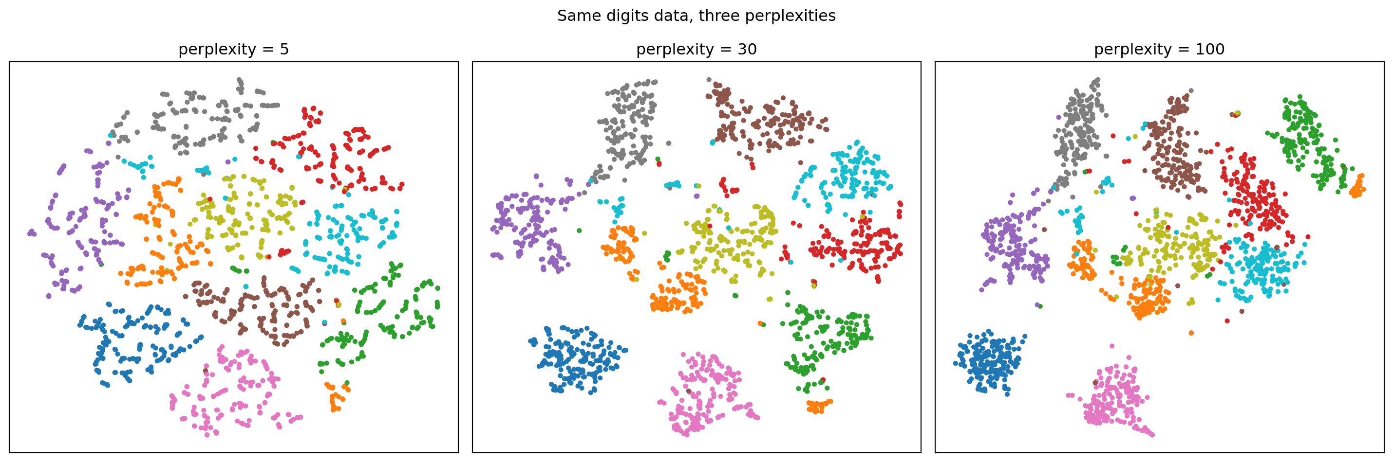
Perplexity is the single most consequential knob. It sets the scale at which the algorithm looks for structure.
low perplexity  (5)   emphasizes very local structure,
                      many small fragmented clusters, noisy
mid perplexity  (30)  the common default, balanced
high perplexity (100) emphasizes broader structure,
                      merges fine clusters, smoother layout
We can see this directly. The cell below runs t-SNE on the digits dataset at three perplexities, after reducing to thirty principal components, and shows how the scale of structure shifts.
The original authors suggest values between 5 and 50 as typical, and a rule of thumb is that perplexity should be smaller than the number of points. When the dataset is small, a perplexity that approaches the sample size makes every point a neighbor of every other and the notion of local structure dissolves. Because the result depends on this choice, no single t-SNE plot is definitive. A responsible analysis inspects several perplexities and trusts only structure that persists across them.
145.4 4. Optimizing the KL Objective
145.4.1 4.1 Gradient Descent with Momentum
The cost \(C = \mathrm{KL}(P \Vert Q)\) is non-convex in the map coordinates \(\{y_i\}\). There is no closed form. t-SNE minimizes it with gradient descent, almost always augmented with momentum to accelerate progress along consistent directions and to escape shallow local minima:
initialize Y with small random values (or a PCA projection)
for t in 1..T:
    compute Q from current Y
    G = gradient of KL(P || Q)
    Y = Y - learning_rate * G + momentum * (Y_prev - Y_prev2)
The optimization is sensitive. A learning rate that is too small leaves points packed in a single dense blob; a common modern heuristic sets the learning rate to roughly \(N / 12\) so that it scales with the number of points. Initialization also matters more than early treatments acknowledged. Initializing from a PCA projection rather than from random noise gives more reproducible layouts and better preserves the coarse arrangement of clusters.
145.4.2 4.2 Early Exaggeration
A characteristic trick is early exaggeration. During the first phase of optimization, all the high-dimensional affinities \(p_{ij}\) are multiplied by a constant, typically around 4 to 12:
Because the \(q_{ij}\) still sum to one, the map cannot satisfy the inflated affinities, and the effect is to strengthen the attractive forces relative to the repulsive ones. Tight clusters form early and move apart from one another, opening up empty space between them. After this phase the exaggeration is removed and the optimization refines the within-cluster arrangement. Skipping early exaggeration often yields a map where clusters fail to separate and overlap into a hairball.
145.4.3 4.3 Scaling to Large Data
Computing all pairwise affinities is \(O(N^2)\), which is prohibitive for large \(N\). Two ideas make t-SNE practical at scale. First, the high-dimensional affinities are sparsified: only the nearest neighbors of each point, found with an approximate nearest neighbor index, contribute non-negligibly to \(P\), so \(P\) becomes sparse. Second, the repulsive part of the gradient, a sum over all pairs, is approximated. The Barnes-Hut algorithm groups distant points into cells of a quadtree and treats each cell as a single body, reducing the cost to \(O(N \log N)\). Fourier-accelerated interpolation methods, as in the FIt-SNE implementation, push this further to roughly \(O(N)\) and make embeddings of millions of points feasible.
145.5 5. How to Read, and Not Misread, t-SNE Plots
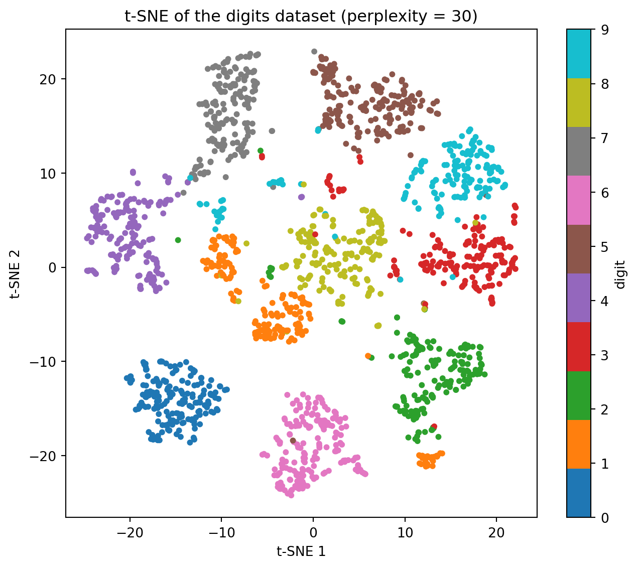
Here is a single t-SNE embedding of the digits dataset at the default perplexity, colored by the true digit label, which serves as the working example for the cautions that follow.
A t-SNE plot is a picture of a non-convex optimization that deliberately sacrifices global geometry to preserve local neighborhoods. Several of its most eye-catching features are not trustworthy. The following points distill the lessons that practitioners learn the hard way, many of them set out clearly in the Distill article by Wattenberg, Viegas, and Johnson.
145.5.1 5.1 Cluster Sizes Are Not Meaningful
The heavy-tailed kernel and the per-point bandwidth together cause t-SNE to equalize density. A tight, dense cluster and a loose, diffuse cluster can render as blobs of nearly the same size in the map. The area a cluster occupies in a t-SNE plot says little about its variance or spread in the original space. Do not compare cluster diameters and conclude anything about relative dispersion.
145.5.2 5.2 Distances Between Clusters Are Not Meaningful
Because the KL objective barely penalizes placing distant points close and places almost no constraint on the relative arrangement of well-separated clusters, the gaps between clusters carry little information. Two clusters far apart on the page are not necessarily more different than two clusters near each other. The global layout of clusters is largely a byproduct of initialization and the optimization path, not of the data. PCA initialization improves this somewhat but does not make inter-cluster distances quantitatively reliable.
145.5.3 5.3 Random-Looking Clumps Can Appear in Noise
Run t-SNE on pure Gaussian noise at a low perplexity and it may still produce apparent clusters. The algorithm is built to find and amplify local neighbor structure, and at small perplexity even chance fluctuations look like neighborhoods. Apparent clusters are only credible when they survive across a range of perplexities and across reruns with different random seeds.
145.5.4 5.4 You Often Need More Than One Plot
Because perplexity sets the scale of analysis and the layout depends on the seed, a single image can mislead. The defensible workflow is to produce several embeddings, varying perplexity over something like 5, 30, and 100, and varying the random seed, and then to report only the structure that is stable. Shapes such as a single cluster pinched into two lobes at one perplexity but merged at another should be treated with suspicion.
145.5.5 5.5 Topology and Shape Can Be Artifacts
t-SNE can tear a connected manifold into pieces, and it can bend a simple shape into a curl that has no counterpart in the data. The curvature of an elongated structure, the presence of a hole, or a filament connecting two clusters may be real or may be an artifact of the force balance and the initialization. When the underlying geometry matters, cross-check against a method with different inductive biases, such as UMAP, or against a direct linear projection like PCA, and trust conclusions only where the methods agree.
145.5.6 5.6 What You Can Trust
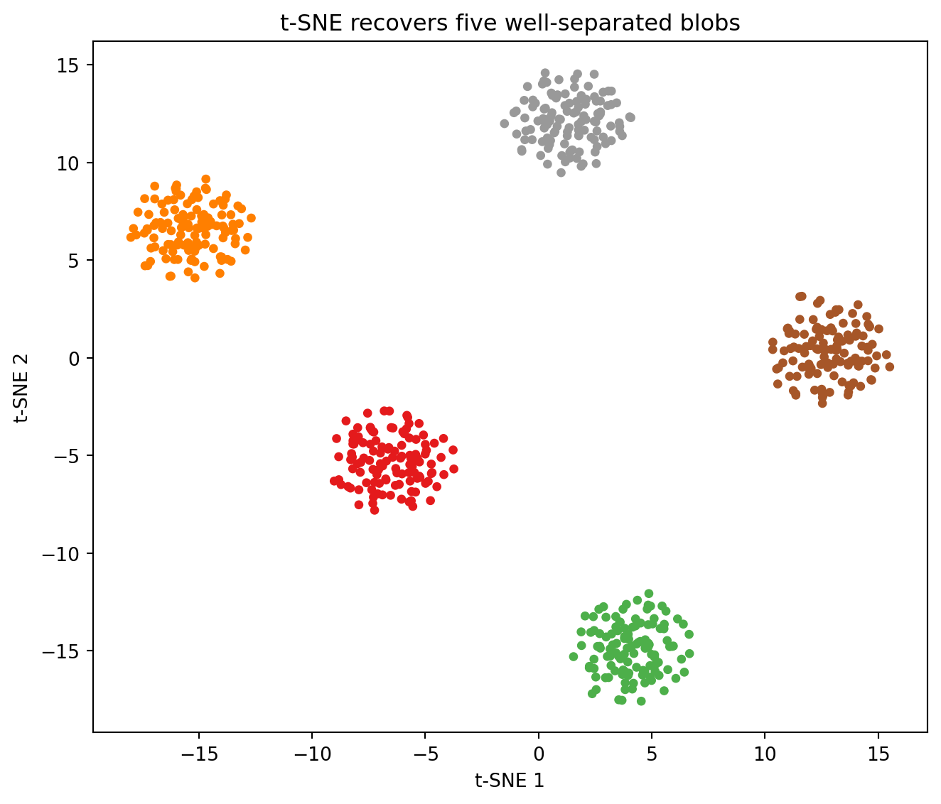
The reliable signal in a t-SNE plot is the existence of well-separated clusters and the membership of points within them. If a group of points consistently embeds together, tightly and apart from the rest, across perplexities and seeds, that grouping reflects genuine local structure in the data. Read t-SNE as a tool for discovering candidate neighborhoods and clusters, to be confirmed by downstream quantitative analysis, and not as a faithful map of high-dimensional geometry.
When clusters genuinely are well separated in the original space, t-SNE recovers them cleanly. The cell below builds five Gaussian blobs in fifty dimensions and embeds them.
The method rewards discipline. A short protocol captures most of the value while avoiding the common traps.
1. standardize or whiten features; reduce to ~50 dims with PCA first
2. choose perplexity sensibly (< N), try several values
3. use PCA initialization for reproducibility
4. use early exaggeration; let the optimization run to convergence
5. scale the learning rate with N (e.g. N/12) on large data
6. rerun with multiple seeds; keep only stable structure
7. never read cluster size, inter-cluster distance, or
   global shape as quantitative facts
Reducing to roughly 50 principal components before running t-SNE is standard practice. It suppresses noise, speeds up the nearest-neighbor search, and rarely discards structure that t-SNE could have used. With these precautions, t-SNE is an excellent instrument for the one thing it was designed to do, which is to reveal local neighborhood structure that high-dimensional data would otherwise hide.
145.7 7. Summary
t-SNE converts pairwise distances into neighbor probabilities, then finds a low-dimensional map whose neighbor probabilities match the originals under a KL divergence. The per-point Gaussian bandwidth, fixed by perplexity, sets the scale of locality. The Student t kernel in the map solves the crowding problem by letting moderately distant points spread apart, and its polynomial tail also yields a well-behaved gradient. Optimization is non-convex gradient descent with momentum, early exaggeration, and, at scale, Barnes-Hut or interpolation-based approximations. The resulting plots are trustworthy about cluster membership and the existence of separated groups, and untrustworthy about cluster size, inter-cluster distance, and global shape. Used with multiple perplexities and seeds, and cross-checked against other methods, t-SNE is a powerful lens; used naively, it invites confident conclusions about structure that is not there.
145.8 References
Hinton, G. and Roweis, S. (2002). Stochastic Neighbor Embedding. Advances in Neural Information Processing Systems 15. https://papers.nips.cc/paper/2276-stochastic-neighbor-embedding
van der Maaten, L. and Hinton, G. (2008). Visualizing Data using t-SNE. Journal of Machine Learning Research 9, 2579-2605. https://www.jmlr.org/papers/v9/vandermaaten08a.html
van der Maaten, L. (2014). Accelerating t-SNE using Tree-Based Algorithms. Journal of Machine Learning Research 15, 3221-3245. https://www.jmlr.org/papers/v15/vandermaaten14a.html
Wattenberg, M., Viegas, F., and Johnson, I. (2016). How to Use t-SNE Effectively. Distill. https://distill.pub/2016/misread-tsne/
Linderman, G. C., Rachh, M., Hoskins, J. G., Steinerberger, S., and Kluger, Y. (2019). Fast interpolation-based t-SNE for improved visualization of single-cell RNA-seq data. Nature Methods 16, 243-245. https://www.nature.com/articles/s41592-018-0308-4
Kobak, D. and Berens, P. (2019). The art of using t-SNE for single-cell transcriptomics. Nature Communications 10, 5416. https://www.nature.com/articles/s41467-019-13056-x
Belkina, A. C. et al. (2019). Automated optimized parameters for t-SNE improve visualization and analysis of large datasets. Nature Communications 10, 5415. https://www.nature.com/articles/s41467-019-13055-z
Source Code
# t-SNE: Theory and Practicet-distributed stochastic neighbor embedding (t-SNE) is the workhorse of high-dimensional data visualization. Given a set of points in a space of hundreds or thousands of dimensions, it produces a two-dimensional or three-dimensional scatter plot in which similar points sit close together and dissimilar points sit apart. The method appears in single-cell genomics, in the inspection of neural network representations, and in nearly any setting where a practitioner wants to look at structure that no scatter plot of raw coordinates could reveal.The appeal of t-SNE is also its danger. The plots it produces are seductive, and they are easy to over-read. This chapter develops the method from its probabilistic foundations so that you understand exactly what the optimization is doing, why the t-distributed kernel matters, what perplexity controls, and, crucially, which features of a t-SNE plot carry information and which are artifacts of the algorithm.## 1. From Distances to Neighbor Probabilities### 1.1 The Stochastic Neighbor Embedding ObjectiveThe ancestor of t-SNE is stochastic neighbor embedding (SNE), introduced by Hinton and Roweis in 2002. The central idea is to convert geometric relationships into probability distributions and then to match a low-dimensional distribution to a high-dimensional one.In the original space, for each point $x_i$ we define a conditional probability that $x_i$ would pick $x_j$ as its neighbor, assuming neighbors are sampled in proportion to a Gaussian density centered on $x_i$:$$p_{j \mid i} = \frac{\exp\!\left(-\lVert x_i - x_j \rVert^2 / 2\sigma_i^2\right)}{\sum_{k \neq i} \exp\!\left(-\lVert x_i - x_k \rVert^2 / 2\sigma_i^2\right)}, \qquad p_{i \mid i} = 0 .$$The bandwidth $\sigma_i$ varies per point and is set by the perplexity constraint discussed in Section 2. Each row of the matrix $p_{j \mid i}$ is a probability distribution over the other points: it encodes who point $i$ considers a likely neighbor.In the low-dimensional map we place points $y_i$ and define an analogous distribution $q_{j \mid i}$. Original SNE used a Gaussian there too:$$q_{j \mid i} = \frac{\exp\!\left(-\lVert y_i - y_j \rVert^2\right)}{\sum_{k \neq i} \exp\!\left(-\lVert y_i - y_k \rVert^2\right)} .$$The map is good when $q_{j \mid i}$ matches $p_{j \mid i}$ for every $i$. SNE measures the mismatch with a sum of Kullback-Leibler divergences, one per point:$$C = \sum_i \mathrm{KL}\!\left(P_i \,\Vert\, Q_i\right) = \sum_i \sum_j p_{j \mid i} \log \frac{p_{j \mid i}}{q_{j \mid i}} .$$The asymmetry of the KL divergence is worth pausing on. The cost pays a large penalty when $p_{j \mid i}$ is large but $q_{j \mid i}$ is small, that is, when two points that are neighbors in the original space are placed far apart in the map. It pays only a small penalty when $p_{j \mid i}$ is small but $q_{j \mid i}$ is large, that is, when two distant points are placed close together. SNE therefore preserves local structure at the expense of global structure by design. This is a feature, not an accident, and it explains much of how the final plots behave.### 1.2 Symmetrizing the Problemt-SNE, introduced by van der Maaten and Hinton in 2008, makes two changes to SNE. The first is to replace the collection of conditional distributions with a single joint distribution over pairs. Rather than minimize a separate KL term per point, t-SNE defines symmetric high-dimensional affinities$$p_{ij} = \frac{p_{j \mid i} + p_{i \mid j}}{2N},$$where $N$ is the number of points. The explicit symmetrization, rather than a direct Gaussian on pairwise distances, guarantees that $\sum_j p_{ij} > 1/(2N)$ for every $i$. This ensures that even an outlier, which all other points consider a poor neighbor, still contributes meaningfully to the cost and cannot be ignored during optimization.The objective collapses to a single divergence between joint distributions:$$C = \mathrm{KL}\!\left(P \,\Vert\, Q\right) = \sum_{i \neq j} p_{ij} \log \frac{p_{ij}}{q_{ij}} .$$The second change, the choice of $q_{ij}$, is the heart of the method and the subject of the next section.## 2. The t-Distributed Kernel and the Crowding Problem### 2.1 Why Gaussians CrowdConsider a cluster of points that genuinely live on a low-dimensional manifold inside a high-dimensional space. In ten dimensions there is a great deal of room: many points can all be roughly equidistant from a central point, each occupying its own direction. When we try to reproduce those same pairwise distances in two dimensions, there simply is not enough area. The volume of a ball of radius $r$ grows like $r^d$, so as $d$ shrinks the periphery that was available in high dimensions cannot be matched in the plane.The consequence, in a Gaussian-to-Gaussian map, is that moderately distant points get pulled inward. Points that should sit at intermediate distance are crushed toward the center of their cluster, clusters smear into one another, and the map degenerates into a single ball. Van der Maaten and Hinton named this the crowding problem.### 2.2 The Heavy-Tailed Fixt-SNE addresses crowding by giving the low-dimensional similarities a heavy tail. Instead of a Gaussian, the map uses a Student t-distribution with one degree of freedom, which is the Cauchy distribution:$$q_{ij} = \frac{\left(1 + \lVert y_i - y_j \rVert^2\right)^{-1}}{\sum_{k \neq l} \left(1 + \lVert y_k - y_l \rVert^2\right)^{-1}} .$$The Cauchy kernel $(1 + d^2)^{-1}$ decays polynomially rather than exponentially. To produce a similarity $q_{ij}$ that matches a small high-dimensional affinity $p_{ij}$, a heavy-tailed kernel requires a much larger map distance than a Gaussian would. In effect, moderately dissimilar points are granted permission to spread far apart in the plane without incurring much cost, which relieves the crowding pressure and lets clusters separate cleanly.There is a second, computational gift. The gradient of the t-SNE cost has a clean form:$$\frac{\partial C}{\partial y_i} = 4 \sum_{j \neq i} \left(p_{ij} - q_{ij}\right) \left(1 + \lVert y_i - y_j \rVert^2\right)^{-1} \left(y_i - y_j\right) .$$The same factor $(1 + \lVert y_i - y_j \rVert^2)^{-1}$ that defines the kernel reappears in the gradient and damps the force between points that are already far apart. The dynamics resemble a physical system of springs in which attractive and repulsive forces between points reach an equilibrium configuration, and that configuration is the embedding.### 2.3 Reading the Kernel as ForcesIt helps to split the gradient into an attractive part driven by $p_{ij}$ and a repulsive part driven by $q_{ij}$. Points that are neighbors in the original data attract; all pairs of points in the map repel, with the repulsion normalized across the whole map. The choice of degrees of freedom in the Student t tail tunes the balance. One degree of freedom is the standard, but variants that increase the tail heaviness for very high-dimensional inputs exist and can sharpen cluster separation further.## 3. Perplexity and the Per-Point Bandwidth### 3.1 What Perplexity MeansThe bandwidth $\sigma_i$ in the high-dimensional kernel is not a free global constant. It is chosen separately for each point so that the resulting conditional distribution $P_i$ has a fixed perplexity. Perplexity is defined through the Shannon entropy $H(P_i) = -\sum_j p_{j \mid i} \log_2 p_{j \mid i}$:$$\mathrm{Perp}(P_i) = 2^{H(P_i)} .$$Perplexity can be read as a smooth measure of the effective number of neighbors. A perplexity of 30 means each point's neighbor distribution behaves roughly as if it spread its probability over 30 neighbors. For each point, t-SNE performs a binary search over $\sigma_i$ until the conditional distribution attains the target perplexity. In a dense region $\sigma_i$ comes out small, in a sparse region it comes out large, so the same effective neighbor count is achieved everywhere. This adaptivity is why t-SNE handles data with varying local density gracefully.### 3.2 The Practical Effect of PerplexityPerplexity is the single most consequential knob. It sets the scale at which the algorithm looks for structure.```textlow perplexity (5) emphasizes very local structure, many small fragmented clusters, noisymid perplexity (30) the common default, balancedhigh perplexity (100) emphasizes broader structure, merges fine clusters, smoother layout```We can see this directly. The cell below runs t-SNE on the digits dataset at three perplexities, after reducing to thirty principal components, and shows how the scale of structure shifts.```{python}import numpy as npimport matplotlib.pyplot as pltfrom sklearn.datasets import load_digitsfrom sklearn.manifold import TSNEfrom sklearn.preprocessing import StandardScalerfrom sklearn.decomposition import PCAdigits = load_digits()X = PCA(n_components=30, random_state=0).fit_transform( StandardScaler().fit_transform(digits.data))perplexities = [5, 30, 100]fig, axes = plt.subplots(1, 3, figsize=(15, 5))for ax, perp inzip(axes, perplexities): emb = TSNE( n_components=2, perplexity=perp, init="pca", max_iter=400, random_state=0, ).fit_transform(X) ax.scatter(emb[:, 0], emb[:, 1], c=digits.target, cmap="tab10", s=8) ax.set_title(f"perplexity = {perp}") ax.set_xticks([]) ax.set_yticks([])fig.suptitle("Same digits data, three perplexities")plt.tight_layout()plt.show()```The original authors suggest values between 5 and 50 as typical, and a rule of thumb is that perplexity should be smaller than the number of points. When the dataset is small, a perplexity that approaches the sample size makes every point a neighbor of every other and the notion of local structure dissolves. Because the result depends on this choice, no single t-SNE plot is definitive. A responsible analysis inspects several perplexities and trusts only structure that persists across them.## 4. Optimizing the KL Objective### 4.1 Gradient Descent with MomentumThe cost $C = \mathrm{KL}(P \Vert Q)$ is non-convex in the map coordinates $\{y_i\}$. There is no closed form. t-SNE minimizes it with gradient descent, almost always augmented with momentum to accelerate progress along consistent directions and to escape shallow local minima:```textinitialize Y with small random values (or a PCA projection)for t in 1..T: compute Q from current Y G = gradient of KL(P || Q) Y = Y - learning_rate * G + momentum * (Y_prev - Y_prev2)```The optimization is sensitive. A learning rate that is too small leaves points packed in a single dense blob; a common modern heuristic sets the learning rate to roughly $N / 12$ so that it scales with the number of points. Initialization also matters more than early treatments acknowledged. Initializing from a PCA projection rather than from random noise gives more reproducible layouts and better preserves the coarse arrangement of clusters.### 4.2 Early ExaggerationA characteristic trick is early exaggeration. During the first phase of optimization, all the high-dimensional affinities $p_{ij}$ are multiplied by a constant, typically around 4 to 12:$$p_{ij} \leftarrow \alpha \, p_{ij}, \qquad \alpha > 1 .$$Because the $q_{ij}$ still sum to one, the map cannot satisfy the inflated affinities, and the effect is to strengthen the attractive forces relative to the repulsive ones. Tight clusters form early and move apart from one another, opening up empty space between them. After this phase the exaggeration is removed and the optimization refines the within-cluster arrangement. Skipping early exaggeration often yields a map where clusters fail to separate and overlap into a hairball.### 4.3 Scaling to Large DataComputing all pairwise affinities is $O(N^2)$, which is prohibitive for large $N$. Two ideas make t-SNE practical at scale. First, the high-dimensional affinities are sparsified: only the nearest neighbors of each point, found with an approximate nearest neighbor index, contribute non-negligibly to $P$, so $P$ becomes sparse. Second, the repulsive part of the gradient, a sum over all pairs, is approximated. The Barnes-Hut algorithm groups distant points into cells of a quadtree and treats each cell as a single body, reducing the cost to $O(N \log N)$. Fourier-accelerated interpolation methods, as in the FIt-SNE implementation, push this further to roughly $O(N)$ and make embeddings of millions of points feasible.## 5. How to Read, and Not Misread, t-SNE PlotsHere is a single t-SNE embedding of the digits dataset at the default perplexity, colored by the true digit label, which serves as the working example for the cautions that follow.```{python}import numpy as npimport matplotlib.pyplot as pltfrom sklearn.datasets import load_digitsfrom sklearn.manifold import TSNEfrom sklearn.preprocessing import StandardScalerfrom sklearn.decomposition import PCAdigits = load_digits()X = StandardScaler().fit_transform(digits.data)X = PCA(n_components=30, random_state=0).fit_transform(X)emb = TSNE( n_components=2, perplexity=30, init="pca", max_iter=400, random_state=0,).fit_transform(X)fig, ax = plt.subplots(figsize=(7, 6))sc = ax.scatter(emb[:, 0], emb[:, 1], c=digits.target, cmap="tab10", s=12)ax.set_title("t-SNE of the digits dataset (perplexity = 30)")ax.set_xlabel("t-SNE 1")ax.set_ylabel("t-SNE 2")fig.colorbar(sc, ax=ax, ticks=range(10), label="digit")plt.tight_layout()plt.show()```A t-SNE plot is a picture of a non-convex optimization that deliberately sacrifices global geometry to preserve local neighborhoods. Several of its most eye-catching features are not trustworthy. The following points distill the lessons that practitioners learn the hard way, many of them set out clearly in the Distill article by Wattenberg, Viegas, and Johnson.### 5.1 Cluster Sizes Are Not MeaningfulThe heavy-tailed kernel and the per-point bandwidth together cause t-SNE to equalize density. A tight, dense cluster and a loose, diffuse cluster can render as blobs of nearly the same size in the map. The area a cluster occupies in a t-SNE plot says little about its variance or spread in the original space. Do not compare cluster diameters and conclude anything about relative dispersion.### 5.2 Distances Between Clusters Are Not MeaningfulBecause the KL objective barely penalizes placing distant points close and places almost no constraint on the relative arrangement of well-separated clusters, the gaps between clusters carry little information. Two clusters far apart on the page are not necessarily more different than two clusters near each other. The global layout of clusters is largely a byproduct of initialization and the optimization path, not of the data. PCA initialization improves this somewhat but does not make inter-cluster distances quantitatively reliable.### 5.3 Random-Looking Clumps Can Appear in NoiseRun t-SNE on pure Gaussian noise at a low perplexity and it may still produce apparent clusters. The algorithm is built to find and amplify local neighbor structure, and at small perplexity even chance fluctuations look like neighborhoods. Apparent clusters are only credible when they survive across a range of perplexities and across reruns with different random seeds.### 5.4 You Often Need More Than One PlotBecause perplexity sets the scale of analysis and the layout depends on the seed, a single image can mislead. The defensible workflow is to produce several embeddings, varying perplexity over something like 5, 30, and 100, and varying the random seed, and then to report only the structure that is stable. Shapes such as a single cluster pinched into two lobes at one perplexity but merged at another should be treated with suspicion.### 5.5 Topology and Shape Can Be Artifactst-SNE can tear a connected manifold into pieces, and it can bend a simple shape into a curl that has no counterpart in the data. The curvature of an elongated structure, the presence of a hole, or a filament connecting two clusters may be real or may be an artifact of the force balance and the initialization. When the underlying geometry matters, cross-check against a method with different inductive biases, such as UMAP, or against a direct linear projection like PCA, and trust conclusions only where the methods agree.### 5.6 What You Can TrustThe reliable signal in a t-SNE plot is the existence of well-separated clusters and the membership of points within them. If a group of points consistently embeds together, tightly and apart from the rest, across perplexities and seeds, that grouping reflects genuine local structure in the data. Read t-SNE as a tool for discovering candidate neighborhoods and clusters, to be confirmed by downstream quantitative analysis, and not as a faithful map of high-dimensional geometry.When clusters genuinely are well separated in the original space, t-SNE recovers them cleanly. The cell below builds five Gaussian blobs in fifty dimensions and embeds them.```{python}import numpy as npimport matplotlib.pyplot as pltfrom sklearn.datasets import make_blobsfrom sklearn.manifold import TSNEXb, yb = make_blobs( n_samples=600, n_features=50, centers=5, cluster_std=2.5, random_state=42,)emb = TSNE( n_components=2, perplexity=30, init="pca", max_iter=400, random_state=42,).fit_transform(Xb)fig, ax = plt.subplots(figsize=(7, 6))ax.scatter(emb[:, 0], emb[:, 1], c=yb, cmap="Set1", s=14)ax.set_title("t-SNE recovers five well-separated blobs")ax.set_xlabel("t-SNE 1")ax.set_ylabel("t-SNE 2")plt.tight_layout()plt.show()```## 6. Practical ChecklistThe method rewards discipline. A short protocol captures most of the value while avoiding the common traps.```text1. standardize or whiten features; reduce to ~50 dims with PCA first2. choose perplexity sensibly (< N), try several values3. use PCA initialization for reproducibility4. use early exaggeration; let the optimization run to convergence5. scale the learning rate with N (e.g. N/12) on large data6. rerun with multiple seeds; keep only stable structure7. never read cluster size, inter-cluster distance, or global shape as quantitative facts```Reducing to roughly 50 principal components before running t-SNE is standard practice. It suppresses noise, speeds up the nearest-neighbor search, and rarely discards structure that t-SNE could have used. With these precautions, t-SNE is an excellent instrument for the one thing it was designed to do, which is to reveal local neighborhood structure that high-dimensional data would otherwise hide.## 7. Summaryt-SNE converts pairwise distances into neighbor probabilities, then finds a low-dimensional map whose neighbor probabilities match the originals under a KL divergence. The per-point Gaussian bandwidth, fixed by perplexity, sets the scale of locality. The Student t kernel in the map solves the crowding problem by letting moderately distant points spread apart, and its polynomial tail also yields a well-behaved gradient. Optimization is non-convex gradient descent with momentum, early exaggeration, and, at scale, Barnes-Hut or interpolation-based approximations. The resulting plots are trustworthy about cluster membership and the existence of separated groups, and untrustworthy about cluster size, inter-cluster distance, and global shape. Used with multiple perplexities and seeds, and cross-checked against other methods, t-SNE is a powerful lens; used naively, it invites confident conclusions about structure that is not there.## References1. Hinton, G. and Roweis, S. (2002). Stochastic Neighbor Embedding. Advances in Neural Information Processing Systems 15. https://papers.nips.cc/paper/2276-stochastic-neighbor-embedding2. van der Maaten, L. and Hinton, G. (2008). Visualizing Data using t-SNE. Journal of Machine Learning Research 9, 2579-2605. https://www.jmlr.org/papers/v9/vandermaaten08a.html3. van der Maaten, L. (2014). Accelerating t-SNE using Tree-Based Algorithms. Journal of Machine Learning Research 15, 3221-3245. https://www.jmlr.org/papers/v15/vandermaaten14a.html4. Wattenberg, M., Viegas, F., and Johnson, I. (2016). How to Use t-SNE Effectively. Distill. https://distill.pub/2016/misread-tsne/5. Linderman, G. C., Rachh, M., Hoskins, J. G., Steinerberger, S., and Kluger, Y. (2019). Fast interpolation-based t-SNE for improved visualization of single-cell RNA-seq data. Nature Methods 16, 243-245. https://www.nature.com/articles/s41592-018-0308-46. Kobak, D. and Berens, P. (2019). The art of using t-SNE for single-cell transcriptomics. Nature Communications 10, 5416. https://www.nature.com/articles/s41467-019-13056-x7. Belkina, A. C. et al. (2019). Automated optimized parameters for t-SNE improve visualization and analysis of large datasets. Nature Communications 10, 5415. https://www.nature.com/articles/s41467-019-13055-z