flowchart LR
subgraph Eager["Eager component trained once"]
E1["Encoder or learned metric"]
end
subgraph Store["Stored experience"]
S1["Embedded instances"]
S2["ANN index"]
end
subgraph Lazy["Lazy component per query"]
L1["Embed query"]
L2["Retrieve k nearest"]
L3["Kernel weight by distance"]
L4["Combine neighbors"]
end
E1 --> S1 --> S2
L1 --> L2
S2 --> L2
L2 --> L3 --> L4 --> P["Prediction or grounded generation"]
100 Instance-Based Learning
Instance-based learning is the family of methods that defer generalization until a query arrives. Rather than compressing a training set into a fixed set of parameters, these methods keep the data and answer new questions by consulting the most relevant stored examples. This chapter develops the theory and practice of instance-based learning, contrasts it with eager parametric learning, and traces the line that runs from the humble nearest-neighbor rule through locally weighted regression and case-based reasoning to the vector retrieval systems that power modern retrieval-augmented generation.
100.1 1. Lazy Versus Eager Learning
100.1.1 1.1 Two Strategies for Generalization
Every supervised learner faces a choice about when to do its work. An eager learner processes the training set \(\mathcal{D} = \{(x_i, y_i)\}_{i=1}^{n}\) once, fitting a global model with parameters \(\theta\) that summarize the data, and then discards the data. Linear regression, logistic regression, decision trees, and neural networks are eager. A lazy learner stores \(\mathcal{D}\) and does almost nothing at training time. When a query \(x_q\) arrives, it inspects the stored instances near \(x_q\) and constructs an answer on the spot.
The trade is one of when the computation happens and where the model lives. Eager learning pays a large up-front cost and amortizes it across an unlimited number of cheap predictions. Lazy learning pays almost nothing up front but pays per query, because each prediction triggers a search over the data. The eager learner commits to a single global hypothesis; the lazy learner implicitly defines a different local hypothesis for every point in input space.
100.1.2 1.2 Why Locality Matters
The defining property of instance-based methods is that they form a target approximation local to the query. This has a real statistical consequence. A global model must choose a single functional form that fits everywhere, so it trades bias against variance once for the whole domain. A local model can be simple near each query yet collectively represent a function of arbitrary complexity, because the complexity is spread across many local fits rather than packed into one parametric form.
The cost is appetite for data and for distance. Locality is only meaningful if “near” is meaningful, so instance-based learning lives or dies by the metric on the input space. It also suffers acutely from the curse of dimensionality. In high dimensions, almost all pairs of points are roughly equidistant, neighborhoods stop being local, and the notion of a nearby example degrades. Much of the modern story is about restoring meaningful locality in high dimensions through learned representations.
100.2 2. The Nearest-Neighbor Rule
100.2.1 2.1 Definition and Decision Boundary
The \(k\)-nearest-neighbor (\(k\)-NN) rule is the canonical instance-based method. Given a distance \(d(\cdot, \cdot)\) and a query \(x_q\), let \(N_k(x_q)\) be the set of \(k\) training points closest to \(x_q\). For classification, predict the majority label in \(N_k(x_q)\):
\[\hat{y}(x_q) = \arg\max_{c} \sum_{i \in N_k(x_q)} \mathbb{1}[y_i = c].\]
For regression, predict the average of neighbor targets:
\[\hat{y}(x_q) = \frac{1}{k} \sum_{i \in N_k(x_q)} y_i.\]
With \(k = 1\) the rule partitions input space into the Voronoi cells of the training points, and the decision boundary is piecewise linear. As \(k\) grows the boundary smooths, bias rises, and variance falls. The parameter \(k\) is the single knob that controls the bias variance trade and is usually chosen by cross-validation.
100.2.2 2.2 Theoretical Guarantees
The nearest-neighbor rule is not a heuristic; it has firm asymptotic backing. The classic result of Cover and Hart shows that as \(n \to \infty\) the error rate of the 1-NN classifier is bounded above by twice the Bayes error rate \(R^{*}\):
\[R^{*} \leq R_{\text{1-NN}} \leq R^{*}\left(2 - \frac{c}{c-1} R^{*}\right) \leq 2 R^{*},\]
where \(c\) is the number of classes. In words, half of the achievable information is already in the single nearest neighbor. For \(k\)-NN with \(k \to \infty\) and \(k/n \to 0\), the rule is Bayes consistent: its error converges to \(R^{*}\). These results justify the method as a strong, assumption-light baseline.
100.2.3 2.3 The Metric Is the Model
For real-valued features the Minkowski family \(d(x, x') = \left( \sum_j |x_j - x'_j|^p \right)^{1/p}\) covers Euclidean (\(p = 2\)) and Manhattan (\(p = 1\)) distance. Because distance sums over features, scale dominates: a feature measured in thousands swamps one measured in fractions. Standardization or a learned linear transform \(d_M(x, x') = \sqrt{(x - x')^\top M (x - x')}\) with a positive semidefinite \(M\) (metric learning) is usually essential. For text and high-dimensional embeddings, cosine similarity \(\cos(x, x') = \frac{x^\top x'}{\lVert x \rVert \lVert x' \rVert}\) is the common choice, since direction carries more signal than magnitude. The choice of metric encodes essentially all of the inductive bias these methods have.
100.3 3. Distance and Kernel Weighting
100.3.1 3.1 From Voting to Weighting
Plain \(k\)-NN treats the nearest and the \(k\)-th nearest neighbor identically, which throws away information about how near each one is. Distance-weighted nearest neighbor fixes this by weighting each neighbor’s vote or target by a decreasing function of its distance. A natural choice is a kernel \(K\):
\[\hat{y}(x_q) = \frac{\sum_{i} K\!\left(\frac{d(x_q, x_i)}{h}\right) y_i}{\sum_{i} K\!\left(\frac{d(x_q, x_i)}{h}\right)}.\]
This is the Nadaraya Watson kernel regression estimator. The bandwidth \(h\) sets the width of the neighborhood and plays the role that \(k\) played before, controlling smoothness. Common kernels include the Gaussian \(K(u) = e^{-u^2/2}\), the Epanechnikov \(K(u) = \max(0, 1 - u^2)\), and the tricube. With a sufficiently sharp kernel, weighting can replace the hard \(k\) cutoff entirely, using all points but letting distant ones contribute negligibly.
100.3.2 3.2 Bandwidth and the Bias Variance Trade
The bandwidth \(h\) is the dominant hyperparameter. A small \(h\) produces a wiggly, high-variance estimate that tracks noise; a large \(h\) produces a smooth, high-bias estimate that washes out real structure. The optimal bandwidth shrinks with sample size, classically at a rate near \(h \propto n^{-1/5}\) for one-dimensional smoothing. Adaptive schemes set \(h\) per query, for example using the distance to the \(k\)-th neighbor so that neighborhoods stay wide in sparse regions and tight in dense ones. This balanced-neighborhood idea reappears in modern approximate nearest-neighbor indexes.
# Distance-weighted prediction, schematic
neighbors = index.search(x_q, k)
weights   = [kernel(d(x_q, xi) / h) for (xi, yi) in neighbors]
y_hat     = weighted_average([yi for (xi, yi) in neighbors], weights)
100.4 4. Locally Weighted Regression
100.4.1 4.1 Fitting a Local Model Per Query
Kernel regression fits a local constant: it averages neighbor targets. Locally weighted regression (LWR), also called LOESS or LOWESS, goes a step further and fits a local linear or low-degree polynomial model around each query, with points weighted by their kernel distance to \(x_q\). Concretely, at query \(x_q\) we solve a weighted least squares problem:
\[\beta(x_q) = \arg\min_{\beta} \sum_{i=1}^{n} K\!\left(\frac{d(x_q, x_i)}{h}\right) \left( y_i - \beta^\top \phi(x_i) \right)^2,\]
where \(\phi\) is a low-order polynomial basis, often \(\phi(x) = [1, x]\). The prediction is \(\hat{y}(x_q) = \beta(x_q)^\top \phi(x_q)\). Because a new weighted regression is solved for every query, the model is genuinely lazy: there is no global \(\beta\), only a field of local ones.
100.4.2 4.2 The Weighted Normal Equations
The local objective is an ordinary weighted least squares problem, so it has a closed form. Stack the basis rows into the design matrix \(\Phi \in \mathbb{R}^{n \times p}\) with \(\Phi_{i\cdot} = \phi(x_i)^\top\), collect the targets in \(y \in \mathbb{R}^n\), and place the kernel weights on the diagonal of \(W(x_q) = \operatorname{diag}\!\big(w_1, \dots, w_n\big)\) with \(w_i = K\!\big(d(x_q, x_i)/h\big)\). The weighted residual sum of squares is
\[J(\beta) = (y - \Phi\beta)^\top W (y - \Phi\beta).\]
Setting the gradient to zero,
\[\nabla_\beta J = -2\,\Phi^\top W (y - \Phi\beta) = 0 \;\Longrightarrow\; \Phi^\top W \Phi\, \beta = \Phi^\top W y,\]
gives the weighted normal equations, whose solution is
\[\beta(x_q) = \left( \Phi^\top W(x_q)\, \Phi \right)^{-1} \Phi^\top W(x_q)\, y.\]
Because \(W\) depends on \(x_q\) through the kernel, \(\beta\) is a function of the query, not a fixed vector. The prediction is linear in the training targets: writing \(\phi_q = \phi(x_q)\),
\[\hat{y}(x_q) = \phi_q^\top \left( \Phi^\top W \Phi \right)^{-1} \Phi^\top W\, y = \ell(x_q)^\top y, \qquad \ell(x_q)^\top = \phi_q^\top \left( \Phi^\top W \Phi \right)^{-1} \Phi^\top W.\]
The row vector \(\ell(x_q)\) is the equivalent kernel or smoother weights, and \(\sum_i \ell_i(x_q) = 1\) exactly for a local linear fit, which is precisely the property that removes the boundary bias of the Nadaraya Watson average. When the local design is rank deficient, as happens when the neighborhood holds too few effective points, the inverse is replaced by a ridge-regularized form \((\Phi^\top W \Phi + \lambda I)^{-1}\).
A useful special case recovers Section 3. If \(\phi(x) = [1]\) is the constant basis, then \(\Phi^\top W \Phi = \sum_i w_i\), \(\Phi^\top W y = \sum_i w_i y_i\), and
\[\hat{y}(x_q) = \frac{\sum_i w_i y_i}{\sum_i w_i},\]
the Nadaraya Watson kernel-weighted average. Local linear regression is therefore the strict generalization that adds a slope term.
100.4.3 4.3 Bandwidth as a Bias Variance Dial
The bandwidth \(h\) inside \(w_i = K(d/h)\) controls the effective size of the neighborhood and so sets the bias variance balance. A standard expansion for local linear smoothing of a twice-differentiable target \(m(x)\) with a symmetric kernel gives, at an interior point,
\[\operatorname{bias}\!\big(\hat{m}(x)\big) \approx \tfrac{1}{2}\, h^2\, \mu_2(K)\, m''(x), \qquad \operatorname{var}\!\big(\hat{m}(x)\big) \approx \frac{\sigma^2\, R(K)}{n\,h\,p(x)},\]
where \(\mu_2(K) = \int u^2 K(u)\,du\), \(R(K) = \int K(u)^2\,du\), \(\sigma^2\) is the noise variance, and \(p(x)\) is the density of inputs. Squared bias grows like \(h^4\) while variance shrinks like \(1/(nh)\), so the mean squared error \(\propto h^4 + 1/(nh)\) is minimized at the classic rate
\[h^\star \propto n^{-1/5}, \qquad \text{giving } \operatorname{MSE} \propto n^{-4/5}.\]
Small \(h\) means narrow kernels, few effective neighbors, low bias and high variance, a wiggly fit that chases noise; large \(h\) means wide kernels, many neighbors, high bias and low variance, a fit that flattens real curvature. The Python section below makes this trade visible by sweeping \(h\) and plotting the resulting fits.
100.4.4 4.4 Why Local Linear Beats Local Constant
Local linear fitting corrects a well-known flaw of kernel averaging: bias at the boundary of the data and in regions where the true function has a strong slope. A local constant estimator is pulled toward whichever side has more neighbors, producing systematic bias near edges. A local linear fit captures the slope and largely removes this first-order bias, which is why LOESS is the default smoother in exploratory data analysis. The price is more computation per query and more sensitivity to sparse neighborhoods, where the weighted design matrix can become ill conditioned and may need ridge regularization.
100.4.5 4.5 Practical Notes
LWR is excellent for smoothing scatter plots, building calibration curves, and modeling smoothly varying responses where a single global form is unjustified. It scales poorly to high dimensions because the local neighborhood empties out, and it requires the full training set at prediction time. In control and robotics it has a long history under the name locally weighted learning, where local linear models of system dynamics are fit on demand around the current state.
100.5 5. Case-Based Reasoning
100.5.1 5.1 The Knowledge-Level View
Case-based reasoning (CBR) is instance-based learning lifted from feature vectors to structured experiences. A case is a rich record of a problem and its solution: a past lawsuit and its ruling, a help-desk ticket and its resolution, a medical presentation and its treatment. CBR solves a new problem by recalling similar past cases and adapting their solutions. It is the explicit cognitive model behind much of human expert reasoning, and it remains the architecture of choice when examples are structured objects rather than points in \(\mathbb{R}^d\).
100.5.2 5.2 The Four-R Cycle
The standard CBR process, due to Aamodt and Plaza, is the cycle of Retrieve, Reuse, Revise, and Retain.
- Retrieve the cases most similar to the new problem, using a domain similarity measure over structured features.
- Reuse their solutions, either directly or as a starting point.
- Revise the proposed solution by adapting it to the new context and testing it.
- Retain the new problem and its verified solution as a case for future use.
The Retain step makes CBR a learning system: the case base grows with experience, and competence improves without retraining a model. Similarity in CBR is rarely a simple Euclidean distance; it is a weighted aggregation of local similarities over heterogeneous attributes, often hand designed with domain knowledge, and adaptation is the hard, knowledge-intensive part.
100.5.3 5.3 Strengths and Limits
CBR shines where solutions are reusable, where the domain is hard to model with a closed-form function, and where explanation matters, because pointing to a precedent is inherently interpretable. Its weaknesses mirror those of all lazy methods: a large case base is expensive to search, retrieval quality depends entirely on the similarity measure, and adaptation can require substantial engineering. The recent revival of CBR comes from pairing its retrieve-and-reuse skeleton with neural similarity and neural adaptation.
100.6 6. The Connection to Modern Retrieval
100.6.1 6.1 Embeddings Restore Meaningful Locality
The fatal weakness of classical instance-based learning was the metric. Raw pixels, bag-of-words counts, and other surface features give distances that do not track semantic similarity, and in high dimensions they collapse. Learned representations change the picture. An encoder \(f_\theta\) maps inputs to vectors so that semantically similar items land near each other, and nearest-neighbor search in that embedding space recovers exactly the locality that classical methods assumed but could not deliver. Crucially, the eager work of representation learning and the lazy work of neighbor search now cooperate: a network is trained once to define the geometry, and prediction is a search.
100.6.2 6.2 Approximate Nearest Neighbors at Scale
Exact nearest-neighbor search costs \(O(n)\) per query, which is untenable for billions of vectors. Approximate nearest-neighbor (ANN) indexes trade a small accuracy loss for orders-of-magnitude speedups. Tree and hashing methods (KD-trees, locality-sensitive hashing) gave way to graph-based indexes, most prominently Hierarchical Navigable Small World (HNSW), which builds a navigable multi-layer proximity graph and answers queries in roughly logarithmic time. Product quantization compresses vectors so that massive collections fit in memory. These engines, exposed through vector databases, are the industrial form of the nearest-neighbor rule.
100.6.3 6.3 Retrieval-Augmented Generation and k-NN Language Models
Modern large language models are eager learners par excellence, with their knowledge baked into fixed weights. Retrieval-augmented generation (RAG) bolts an instance-based memory onto this eager core: at inference time the system embeds the query, retrieves the nearest passages from a corpus, and conditions generation on them. This is the four-R cycle in a new guise, retrieve and reuse, with the language model performing revision. It lets a frozen model use fresh, private, or domain-specific knowledge without retraining, and it grounds answers in citable sources.
The same spirit appears inside the prediction itself. The \(k\)-NN language model interpolates a parametric model’s next-token distribution with a distribution formed by retrieving the nearest contexts from a datastore of cached hidden states:
\[p(y \mid x) = \lambda \, p_{\text{kNN}}(y \mid x) + (1 - \lambda) \, p_{\text{LM}}(y \mid x).\]
Here \(p_{\text{kNN}}\) is a distance-weighted vote over the targets of the retrieved neighbors, exactly the distance-weighted nearest-neighbor estimator of Section 3, operating in the model’s own representation space. Few-shot in-context learning is yet another instance-based reading: retrieved examples placed in the prompt act as a local training set for a single query, generalization deferred to inference time.
100.6.4 6.4 The Unifying Picture
Across these systems one pattern recurs. An eager component learns a representation or a metric; a lazy component answers each query by finding and combining nearby stored instances. The classical questions return unchanged: how to define distance, how to weight neighbors, how many to use, and how to search efficiently. Instance-based learning, far from being a historical baseline, is the operating principle of the retrieval layer that now sits beneath much of applied AI.
The unifying pattern, eager metric plus lazy retrieval, can be drawn as a single pipeline that the classical and modern systems share.
| Node | Detail |
|---|---|
| Encoder or learned metric | Encoder \(f_\theta\) or learned metric \(M\) |
| ANN index | Approximate nearest neighbor index such as HNSW or PQ |
| Embed query | Embed the query point \(x_q\) |
| Combine neighbors | Combine by vote, average, or local fit |
100.7 7. A Locally Weighted Regression Laboratory
The following lab builds a one-dimensional locally weighted regression from the weighted normal equations of Section 4.2, sweeps the bandwidth to show the bias variance trade of Section 4.3, verifies the equivalent kernel sums to one, and confirms the constant-basis special case reduces to the Nadaraya Watson average. It uses only open-source tools: NumPy, scikit-learn, pandas, Matplotlib, and SymPy.
Code
import numpy as np
import pandas as pd
import matplotlib.pyplot as plt
import sympy as sp
from sklearn.metrics import mean_squared_error
rng = np.random.default_rng(7)
# Ground-truth function with varying curvature, plus noise.
def true_f(x):
return np.sin(2.0 * x) + 0.3 * x
n = 120
x = np.sort(rng.uniform(0.0, 6.0, size=n))
sigma = 0.25
y = true_f(x) + rng.normal(0.0, sigma, size=n)
def gaussian_kernel(dist, h):
return np.exp(-0.5 * (dist / h) ** 2)
def lwr_predict(x_train, y_train, x_query, h, degree=1, ridge=1e-8):
"""Local polynomial regression via the weighted normal equations.
Returns predictions and, for each query, the equivalent-kernel weight row.
"""
x_train = np.asarray(x_train, float)
y_train = np.asarray(y_train, float)
x_query = np.atleast_1d(np.asarray(x_query, float))
preds = np.empty(x_query.shape[0])
ell_sums = np.empty(x_query.shape[0])
# Polynomial basis phi(x) = [1, x, x^2, ...].
def basis(xv):
return np.vstack([xv ** d for d in range(degree + 1)]).T
Phi = basis(x_train) # n x p
for j, xq in enumerate(x_query):
w = gaussian_kernel(np.abs(x_train - xq), h) # kernel weights
W = Phi * w[:, None] # W Phi (rows scaled)
A = Phi.T @ W + ridge * np.eye(Phi.shape[1]) # Phi^T W Phi (+ ridge)
b = Phi.T @ (w * y_train) # Phi^T W y
beta = np.linalg.solve(A, b)
phi_q = basis(np.array([xq]))[0]
preds[j] = phi_q @ beta
# Equivalent kernel ell(x_q)^T = phi_q^T (Phi^T W Phi)^-1 Phi^T W
ell = phi_q @ np.linalg.solve(A, Phi.T * w[None, :])
ell_sums[j] = ell.sum()
return preds, ell_sums
xs = np.linspace(0.05, 5.95, 300)
bandwidths = [0.10, 0.30, 0.80, 2.00]
# ---- Figure 1: local linear fits at several bandwidths ----
fig1, axes = plt.subplots(2, 2, figsize=(11, 7), sharex=True, sharey=True)
rows = []
for ax, h in zip(axes.ravel(), bandwidths):
yhat_grid, ell_sums = lwr_predict(x, y, xs, h, degree=1)
yhat_train, _ = lwr_predict(x, y, x, h, degree=1)
mse_fit = mean_squared_error(true_f(xs), yhat_grid)
ax.scatter(x, y, s=14, alpha=0.4, color="tab:gray", label="data")
ax.plot(xs, true_f(xs), "k--", lw=1.5, label="true f")
ax.plot(xs, yhat_grid, color="tab:red", lw=2.0, label=f"LWR h={h}")
ax.set_title(f"bandwidth h = {h:.2f} MSE vs truth = {mse_fit:.3f}")
ax.legend(fontsize=8, loc="upper right")
rows.append({
"bandwidth_h": h,
"mse_vs_truth": mse_fit,
"train_residual_std": float(np.std(y - yhat_train)),
"equiv_kernel_sum_mean": float(np.mean(ell_sums)),
})
fig1.suptitle("Locally weighted linear regression across bandwidths", fontsize=13)
fig1.tight_layout()
# ---- Results table ----
results = pd.DataFrame(rows)
print("Bandwidth sweep results")
print(results.to_string(index=False, float_format=lambda v: f"{v:8.4f}"))
best = results.loc[results["mse_vs_truth"].idxmin()]
print(f"\nBest bandwidth by MSE-vs-truth: h = {best['bandwidth_h']:.2f} "
f"(MSE = {best['mse_vs_truth']:.4f})")
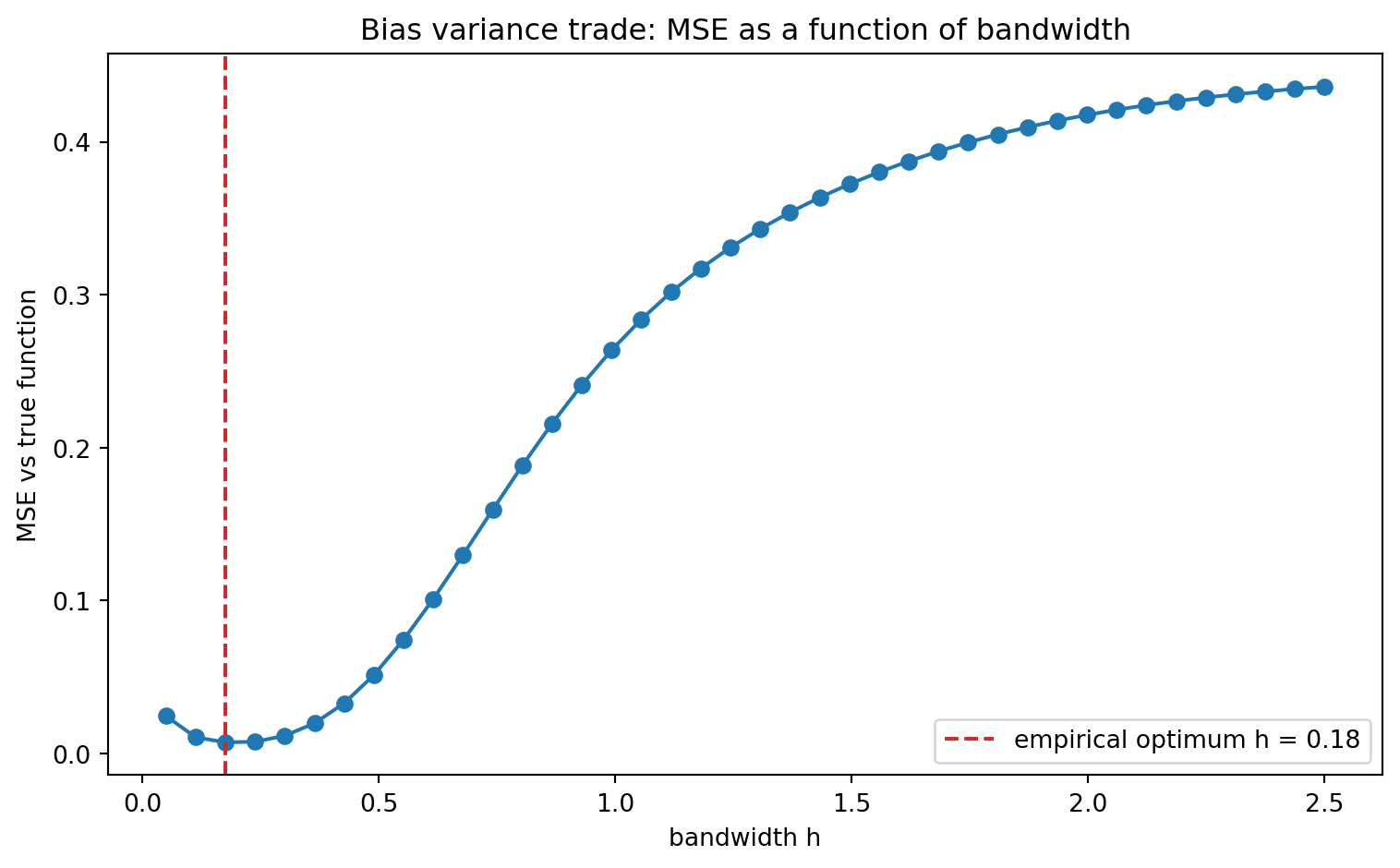
# ---- Figure 2: bias-variance curve over a fine bandwidth grid ----
h_grid = np.linspace(0.05, 2.5, 40)
mse_curve = []
for h in h_grid:
yhat_grid, _ = lwr_predict(x, y, xs, h, degree=1)
mse_curve.append(mean_squared_error(true_f(xs), yhat_grid))
mse_curve = np.array(mse_curve)
h_opt = h_grid[int(np.argmin(mse_curve))]
fig2, ax2 = plt.subplots(figsize=(8, 5))
ax2.plot(h_grid, mse_curve, "o-", color="tab:blue")
ax2.axvline(h_opt, color="tab:red", ls="--",
label=f"empirical optimum h = {h_opt:.2f}")
ax2.set_xlabel("bandwidth h")
ax2.set_ylabel("MSE vs true function")
ax2.set_title("Bias variance trade: MSE as a function of bandwidth")
ax2.legend()
fig2.tight_layout()
print(f"\nEmpirical optimal bandwidth on fine grid: h = {h_opt:.3f}")
# ---- Numeric check: constant basis (degree 0) == Nadaraya-Watson average ----
h_chk = 0.5
xq_chk = 3.0
nw = (np.sum(gaussian_kernel(np.abs(x - xq_chk), h_chk) * y)
/ np.sum(gaussian_kernel(np.abs(x - xq_chk), h_chk)))
lwr0, _ = lwr_predict(x, y, np.array([xq_chk]), h_chk, degree=0)
print(f"\nConstant-basis LWR at x={xq_chk}: {lwr0[0]:.6f}")
print(f"Nadaraya-Watson average at x={xq_chk}: {nw:.6f}")
print(f"Match: {np.isclose(lwr0[0], nw)}")
# ---- SymPy check: weighted normal equations minimize the WLS objective ----
b0, b1 = sp.symbols("b0 b1", real=True)
# Tiny symbolic dataset with symbolic weights.
xi = [sp.Integer(0), sp.Integer(1), sp.Integer(2)]
yi = [sp.Integer(1), sp.Integer(2), sp.Integer(2)]
wi = [sp.Rational(1, 2), sp.Integer(1), sp.Rational(1, 4)]
J = sum(w * (yv - (b0 + b1 * xv)) ** 2 for xv, yv, w in zip(xi, yi, wi))
sol = sp.solve([sp.diff(J, b0), sp.diff(J, b1)], [b0, b1], dict=True)[0]
Phi_s = sp.Matrix([[1, xv] for xv in xi])
W_s = sp.diag(*wi)
y_s = sp.Matrix(yi)
beta_closed = (Phi_s.T * W_s * Phi_s).inv() * Phi_s.T * W_s * y_s
print("\nSymPy: WLS objective minimizer")
print(f" from gradient = 0 : b0={sol[b0]}, b1={sol[b1]}")
print(f" from normal eqns : b0={sp.nsimplify(beta_closed[0])}, "
f"b1={sp.nsimplify(beta_closed[1])}")
print(f" agree: {sp.simplify(beta_closed[0]-sol[b0])==0 and sp.simplify(beta_closed[1]-sol[b1])==0}")
plt.show()Bandwidth sweep results
bandwidth_h mse_vs_truth train_residual_std equiv_kernel_sum_mean
0.1000 0.0121 0.1992 1.0000
0.3000 0.0115 0.2425 1.0000
0.8000 0.1867 0.5307 1.0000
2.0000 0.4177 0.7283 1.0000
Best bandwidth by MSE-vs-truth: h = 0.30 (MSE = 0.0115)
Empirical optimal bandwidth on fine grid: h = 0.176
Constant-basis LWR at x=3.0: 0.794913
Nadaraya-Watson average at x=3.0: 0.794913
Match: True
SymPy: WLS objective minimizer
from gradient = 0 : b0=6/5, b1=3/5
from normal eqns : b0=6/5, b1=3/5
agree: True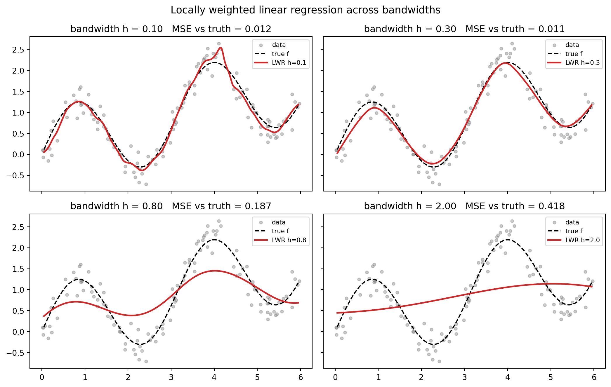
using LinearAlgebra, Random, Statistics, Printf

Random.seed!(7)
true_f(x) = sin(2x) + 0.3x

n = 120
x = sort(6 .* rand(n))
y = true_f.(x) .+ 0.25 .* randn(n)

gkernel(d, h) = exp(-0.5 * (d / h)^2)

# Local polynomial regression via weighted normal equations.
function lwr(xtr, ytr, xq, h; degree=1, ridge=1e-8)
    basis(v) = reduce(hcat, [v .^ d for d in 0:degree])
    Phi = basis(xtr)
    preds = similar(xq)
    for (j, q) in enumerate(xq)
        w = gkernel.(abs.(xtr .- q), h)
        A = Phi' * (w .* Phi) + ridge * I
        b = Phi' * (w .* ytr)
        beta = A \ b
        preds[j] = (basis([q]))[1, :]' * beta
    end
    return preds
end

xs = collect(range(0.05, 5.95, length=300))
for h in (0.10, 0.30, 0.80, 2.00)
    yhat = lwr(x, y, xs, h)
    @printf("h=%.2f  MSE vs truth = %.4f\n", h, mean((true_f.(xs) .- yhat) .^ 2))
end
// Local linear regression (degree 1) via 2x2 weighted normal equations.
// Dependencies: none beyond std. Solves Phi^T W Phi beta = Phi^T W y.
fn gkernel(d: f64, h: f64) -> f64 {
(-0.5 * (d / h).powi(2)).exp()
}
fn lwr_point(x: &[f64], y: &[f64], xq: f64, h: f64) -> f64 {
// Accumulate the 2x2 system [s0 s1; s1 s2] beta = [t0; t1].
let (mut s0, mut s1, mut s2, mut t0, mut t1) = (0.0, 0.0, 0.0, 0.0, 0.0);
for (&xi, &yi) in x.iter().zip(y.iter()) {
let w = gkernel((xi - xq).abs(), h);
s0 += w;
s1 += w * xi;
s2 += w * xi * xi;
t0 += w * yi;
t1 += w * xi * yi;
}
let det = s0 * s2 - s1 * s1 + 1e-12;
let b0 = (s2 * t0 - s1 * t1) / det; // intercept
let b1 = (s0 * t1 - s1 * t0) / det; // slope
b0 + b1 * xq
}
fn true_f(x: f64) -> f64 {
(2.0 * x).sin() + 0.3 * x
}
fn main() {
// Deterministic grid sample (no RNG dependency).
let x: Vec<f64> = (0..120).map(|i| i as f64 * 6.0 / 119.0).collect();
let y: Vec<f64> = x.iter().map(|&xi| true_f(xi)).collect();
for h in [0.10_f64, 0.30, 0.80, 2.00] {
let preds: Vec<f64> = x.iter().map(|&xq| lwr_point(&x, &y, xq, h)).collect();
let mse: f64 = preds
.iter()
.zip(y.iter())
.map(|(p, t)| (p - t).powi(2))
.sum::<f64>()
/ x.len() as f64;
println!("h={:.2} MSE vs truth = {:.4}", h, mse);
}
}100.8 8. Practical Guidance
Choose instance-based methods when the decision boundary is irregular, when data arrives continuously and retraining is costly, when interpretability through precedent is valued, or when a strong baseline is needed quickly. Invest first in the metric or the embedding, because it dominates everything else. Standardize features, learn a metric if labels permit, and prefer distance weighting over hard voting. Tune \(k\) or the bandwidth \(h\) by cross-validation, and watch for the curse of dimensionality by reducing or learning representations before searching. At scale, reach for an ANN index rather than exact search, and accept a small recall loss for a large latency gain. Above all, remember that storing the data is not free: prediction cost, memory, and the staleness of the case base are the standing liabilities of every lazy learner.
100.9 References
- Cover, T. M., and Hart, P. E. “Nearest Neighbor Pattern Classification.” IEEE Transactions on Information Theory, 1967. https://ieeexplore.ieee.org/document/1053964
- Aha, D. W., Kibler, D., and Albert, M. K. “Instance-Based Learning Algorithms.” Machine Learning, 1991. https://link.springer.com/article/10.1007/BF00153759
- Atkeson, C. G., Moore, A. W., and Schaal, S. “Locally Weighted Learning.” Artificial Intelligence Review, 1997. https://link.springer.com/article/10.1023/A:1006559212014
- Cleveland, W. S. “Robust Locally Weighted Regression and Smoothing Scatterplots.” Journal of the American Statistical Association, 1979. https://www.tandfonline.com/doi/abs/10.1080/01621459.1979.10481038
- Aamodt, A., and Plaza, E. “Case-Based Reasoning: Foundational Issues, Methodological Variations, and System Approaches.” AI Communications, 1994. https://www.iiia.csic.es/~enric/papers/AICom.pdf
- Hastie, T., Tibshirani, R., and Friedman, J. “The Elements of Statistical Learning.” Springer, 2009. https://hastie.su.domains/ElemStatLearn/
- Malkov, Y. A., and Yashunin, D. A. “Efficient and Robust Approximate Nearest Neighbor Search Using Hierarchical Navigable Small World Graphs.” IEEE TPAMI, 2020. https://arxiv.org/abs/1603.09320
- Khandelwal, U., Levy, O., Jurafsky, D., Zettlemoyer, L., and Lewis, M. “Generalization through Memorization: Nearest Neighbor Language Models.” ICLR, 2020. https://arxiv.org/abs/1911.00172
- Lewis, P., et al. “Retrieval-Augmented Generation for Knowledge-Intensive NLP Tasks.” NeurIPS, 2020. https://arxiv.org/abs/2005.11401