31 Foundations of Probability

Probability is the mathematics of uncertainty. Almost every modern machine learning system, from a spam filter to a large language model, is at heart a machinery for reasoning about what is likely given what has been observed. To understand why these systems work, why they sometimes fail, and how to improve them, we need a precise account of what probability is. This chapter builds that account from the ground up. We start with the raw ingredients of a random experiment, state the axioms that any sensible notion of probability must obey, and develop the core tools of conditioning, independence, and total probability. Throughout, we connect each idea to the way uncertainty shows up in learning systems.

31.1 1. Sample Spaces and Events

31.1.1 1.1 The Anatomy of a Random Experiment

A probabilistic model begins with an experiment whose outcome is uncertain before it is performed. The set of all possible outcomes is the sample space, denoted $\Omega$. Each individual outcome is an element $\omega \in \Omega$, sometimes called a sample point. The sample space is the universe of possibilities, and everything we can later say about probability is a statement about subsets of this universe.

Consider a single roll of a fair die. The sample space is $\Omega = \{1, 2, 3, 4, 5, 6\}$, a finite set with six elements. If we flip a coin until the first head appears, the sample space is countably infinite, $\Omega = \{H, TH, TTH, TTTH, \ldots\}$. If we measure the time until a hard drive fails, the sample space is the continuous interval $\Omega = [0, \infty)$. These three cases, finite, countably infinite, and uncountable, require slightly different mathematical machinery, but the conceptual picture is the same.

An event is a subset of the sample space, $A \subseteq \Omega$. We say the event $A$ occurs if the realized outcome $\omega$ belongs to $A$. For the die, the event “the roll is even” is $A = \{2, 4, 6\}$. The event “the roll is at least five” is $B = \{5, 6\}$. Events are sets, so the language of set theory becomes the language of events. The union $A \cup B$ is the event that $A$ or $B$ (or both) occur. The intersection $A \cap B$ is the event that both occur. The complement $A^c = \Omega \setminus A$ is the event that $A$ does not occur. The empty set $\varnothing$ is the impossible event, and $\Omega$ itself is the certain event.

Two events are mutually exclusive, or disjoint, when $A \cap B = \varnothing$, meaning they cannot both occur. A collection of events is exhaustive when their union is all of $\Omega$. A collection that is both mutually exclusive and exhaustive forms a partition of the sample space, a notion we will lean on heavily when we reach the law of total probability.

31.1.2 1.2 Why We Need a Sigma-Algebra

It is tempting to declare that every subset of $\Omega$ is an event to which we can assign a probability. For finite and countable sample spaces this works perfectly well. For uncountable sample spaces, such as the real line, it turns out that we cannot consistently assign probabilities to every subset without running into contradictions. The pathological sets that cause trouble are exotic and never arise in practical modeling, but their existence forces us to be careful.

The resolution is to restrict attention to a collection $\mathcal{F}$ of subsets of $\Omega$ that we agree to call events. This collection must be a sigma-algebra (also written $\sigma$-algebra), meaning it satisfies three closure properties:

$\Omega \in \mathcal{F}$.
If $A \in \mathcal{F}$ then its complement $A^c \in \mathcal{F}$ (closure under complementation).
If $A_1, A_2, A_3, \ldots$ is a countable sequence of sets in $\mathcal{F}$, then their union $\bigcup_{i=1}^{\infty} A_i$ also lies in $\mathcal{F}$ (closure under countable unions).

These three properties already force a great deal more. Because $\Omega \in \mathcal{F}$ and $\mathcal{F}$ is closed under complementation, the empty set $\varnothing = \Omega^c$ belongs to $\mathcal{F}$. Closure under countable unions plus De Morgan’s laws gives closure under countable intersections, since \[ \bigcap_{i=1}^{\infty} A_i = \left( \bigcup_{i=1}^{\infty} A_i^c \right)^{\!c}, \] and the right hand side is a complement of a countable union of complements, each step of which stays inside $\mathcal{F}$. Finite unions and intersections follow by padding a finite list with copies of $\varnothing$ or $\Omega$, and set differences $A \setminus B = A \cap B^c$ are covered as well. In short, any event we can construct from countably many basic events by the usual logical operations is itself a legitimate event.

For a finite or countable $\Omega$ we may safely take $\mathcal{F} = 2^{\Omega}$, the power set of all subsets. For $\Omega = \mathbb{R}$ the standard choice is the Borel sigma-algebra $\mathcal{B}(\mathbb{R})$, the smallest sigma-algebra containing every open interval. It contains every set one meets in practice, yet it is a strict subset of the power set, which is exactly what lets a consistent probability measure exist.

The triple $(\Omega, \mathcal{F}, P)$, consisting of a sample space, a sigma-algebra of events, and a probability measure $P$ defined on $\mathcal{F}$, is called a probability space. This is the formal object on which all of probability theory rests. In practice, machine learning practitioners rarely write down the sigma-algebra explicitly. It works quietly in the background, ensuring that quantities like expectations and conditional probabilities are well defined. But knowing it is there clarifies why probability is a theory of measure, not merely a theory of counting.

31.2 2. The Kolmogorov Axioms

31.2.1 2.1 Three Rules That Define Probability

In 1933 Andrey Kolmogorov gave probability theory the rigorous footing it had lacked for centuries by proposing that probability is simply a measure that assigns the value one to the whole space [1]. A probability measure is a function $P : \mathcal{F} \to \mathbb{R}$ satisfying three axioms.

The first axiom is non-negativity. For every event $A \in \mathcal{F}$, \[ P(A) \geq 0 . \] Probabilities are never negative. This reflects the intuition that the chance of something cannot be less than impossible.

The second axiom is normalization. The probability of the entire sample space is one, \[ P(\Omega) = 1 . \] Something in $\Omega$ must happen, and we calibrate certainty to the value one.

The third axiom is countable additivity. If $A_1, A_2, A_3, \ldots$ is a countable collection of pairwise disjoint events, meaning $A_i \cap A_j = \varnothing$ whenever $i \neq j$, then \[ P\!\left(\bigcup_{i=1}^{\infty} A_i\right) = \sum_{i=1}^{\infty} P(A_i) . \] The probability of a union of non-overlapping events is the sum of their individual probabilities. This is the axiom that does the real work, because it lets us decompose complicated events into simpler pieces and add up the parts.

That is the entire foundation. Everything else in probability, every formula and theorem, is a logical consequence of these three statements together with the structure of the probability space.

31.2.2 2.2 Consequences of the Axioms

A handful of useful facts follow immediately, and it is worth seeing them proved rather than merely asserted, because every one is a short deduction from the three axioms.

Finite additivity. Countable additivity implies the finite version. Given disjoint $A_1, \ldots, A_n$, extend the list with $A_{n+1} = A_{n+2} = \cdots = \varnothing$. These remain pairwise disjoint, and since (as shown next) $P(\varnothing) = 0$, the infinite sum collapses to the finite one, giving $P(A_1 \cup \cdots \cup A_n) = \sum_{i=1}^{n} P(A_i)$.

The empty set has probability zero. Take $A_1 = \Omega$ and $A_i = \varnothing$ for $i \ge 2$. These are pairwise disjoint with union $\Omega$, so countable additivity gives $P(\Omega) = P(\Omega) + \sum_{i \ge 2} P(\varnothing)$. Subtracting $P(\Omega)$ leaves $\sum_{i \ge 2} P(\varnothing) = 0$, and since each term is non-negative by the first axiom, $P(\varnothing) = 0$.

The complement rule. Because $A$ and $A^c$ are disjoint and $A \cup A^c = \Omega$, finite additivity and normalization give $P(A) + P(A^c) = P(\Omega) = 1$, hence \[ P(A^c) = 1 - P(A) . \]

Monotonicity. If $A \subseteq B$, then $B$ is the disjoint union of $A$ and $B \setminus A$, so $P(B) = P(A) + P(B \setminus A)$. Non-negativity of the second term yields $P(B) \ge P(A)$: larger events are at least as probable as the smaller events they contain. Applying this with $B = \Omega$ shows $P(A) \le 1$, so together with non-negativity every probability lies in $[0, 1]$.

Inclusion-exclusion for two events. When two events may overlap, naive addition double counts the intersection. To correct for it, decompose both the union and each event into disjoint pieces. Write \[ A \cup B = (A \setminus B) \,\cup\, (A \cap B) \,\cup\, (B \setminus A), \] a union of three pairwise disjoint sets. Finite additivity gives $P(A \cup B) = P(A \setminus B) + P(A \cap B) + P(B \setminus A)$. Separately, $A = (A \setminus B) \cup (A \cap B)$ and $B = (B \setminus A) \cup (A \cap B)$, each a disjoint split, so $P(A \setminus B) = P(A) - P(A \cap B)$ and $P(B \setminus A) = P(B) - P(A \cap B)$. Substituting these in yields the inclusion-exclusion principle, \[ P(A \cup B) = P(A) + P(B) - P(A \cap B) . \] Because $P(A \cap B) \ge 0$, a direct corollary is the union bound, $P(A \cup B) \le P(A) + P(B)$, which extends by induction and then a limiting argument to any countable collection, \[ P\!\left(\bigcup_{i} A_i\right) \le \sum_{i} P(A_i) . \] The union bound is one of the most heavily used tools in the theoretical analysis of machine learning. When proving that a learned model generalizes, we often need to control the probability that any one of many bad events occurs. The union bound lets us bound that combined failure probability by summing the individual failure probabilities, even when the events are dependent in complicated ways. Generalization bounds for finite hypothesis classes are built on exactly this idea [2].

31.2.3 2.3 Interpreting What Probability Means

The axioms tell us how probabilities behave but not what they signify. Two interpretations dominate. The frequentist view holds that the probability of an event is the long-run relative frequency with which it occurs across many independent repetitions of the experiment. The probability that a coin lands heads is the limiting fraction of heads as the number of tosses grows without bound, a statement made precise by the law of large numbers.

The Bayesian view holds that probability is a degree of belief, a numerical measure of how confident a rational agent is in a proposition given the information available. Under this reading we may speak of the probability that a particular email is spam, or that a specific model parameter takes a certain value, even though there is no repeatable experiment in sight. Both interpretations satisfy the same Kolmogorov axioms, so the mathematics is shared even where the philosophy diverges. Machine learning draws on both: frequentist arguments justify why empirical risk minimization works, while Bayesian arguments underpin probabilistic modeling, posterior inference, and the quantification of model uncertainty.

31.3 3. Conditional Probability

31.3.1 3.1 Updating Beliefs in Light of Evidence

The single most important operation in probabilistic reasoning is updating what we believe once we learn something. The conditional probability of $A$ given $B$, written $P(A \mid B)$, is the probability that $A$ occurs under the knowledge that $B$ has occurred. Provided $P(B) > 0$, it is defined by \[ P(A \mid B) = \frac{P(A \cap B)}{P(B)} . \] The intuition is geometric. Learning that $B$ occurred shrinks the relevant universe from all of $\Omega$ down to $B$. Within this smaller universe we ask what fraction of probability mass also falls in $A$. We rescale by dividing through by $P(B)$ so that the conditional probabilities over the restricted space again sum to one. Indeed, $P(\cdot \mid B)$ is itself a perfectly valid probability measure on $\Omega$, satisfying all three Kolmogorov axioms.

Return to the die. Let $A = \{$the roll is even$\} = \{2, 4, 6\}$ and $B = \{$the roll is at least four$\} = \{4, 5, 6\}$. Then $A \cap B = \{4, 6\}$, so \[ P(A \mid B) = \frac{P(\{4, 6\})}{P(\{4, 5, 6\})} = \frac{2/6}{3/6} = \frac{2}{3} . \] Knowing the roll is at least four raises the probability that it is even from one half to two thirds, because two of the three remaining outcomes are even.

31.3.2 3.2 The Chain Rule and Bayes’ Theorem

Rearranging the definition gives the multiplication rule, $P(A \cap B) = P(A \mid B)\, P(B)$. Applied repeatedly it yields the chain rule for the joint probability of a sequence of events, \[ P(A_1 \cap A_2 \cap \cdots \cap A_n) = P(A_1)\, P(A_2 \mid A_1)\, P(A_3 \mid A_1 \cap A_2) \cdots P(A_n \mid A_1 \cap \cdots \cap A_{n-1}) . \] The chain rule is the backbone of autoregressive models. A language model factorizes the probability of a sequence of tokens $w_1, \ldots, w_n$ as $P(w_1) \prod_{t=2}^{n} P(w_t \mid w_1, \ldots, w_{t-1})$, predicting each token conditioned on everything before it. Training such a model amounts to learning these conditional distributions, and generation amounts to sampling from them one step at a time.

The most consequential rearrangement is Bayes’ theorem, which inverts the direction of conditioning, \[ P(A \mid B) = \frac{P(B \mid A)\, P(A)}{P(B)} . \] This formula lets us compute the probability of a hidden cause $A$ given an observed effect $B$ when we know the reverse relationship, the probability of the effect given the cause. In the language of inference, $P(A)$ is the prior, $P(B \mid A)$ is the likelihood, $P(B)$ is the evidence or marginal likelihood, and $P(A \mid B)$ is the posterior. Bayes’ theorem is the engine of probabilistic machine learning, from naive Bayes classifiers to full Bayesian neural networks [3]. A spam filter, for instance, treats the words in a message as evidence and uses Bayes’ theorem to compute the posterior probability that the message is spam given those words.

31.3.3 3.3 The Base Rate Fallacy

Conditional probability is notoriously counterintuitive, and the most common error is to neglect the prior. Suppose a diagnostic test for a disease is ninety nine percent accurate in both directions, yet the disease afflicts only one person in ten thousand. If a randomly chosen person tests positive, the probability they actually have the disease is not ninety nine percent.

Let us work it out exactly, because the worked example ties together every tool in this chapter. Write $D$ for the event of having the disease and $T^{+}$ for a positive test. The given quantities are the prior $P(D) = 0.0001$, the sensitivity $P(T^{+} \mid D) = 0.99$, and the specificity $P(T^{-} \mid D^c) = 0.99$, so the false positive rate is $P(T^{+} \mid D^c) = 0.01$. First compute the evidence by the law of total probability over the partition $\{D, D^c\}$, \[ P(T^{+}) = P(T^{+} \mid D)\, P(D) + P(T^{+} \mid D^c)\, P(D^c) = 0.99 \times 0.0001 + 0.01 \times 0.9999 = 0.010098 . \] Now apply Bayes’ theorem, \[ P(D \mid T^{+}) = \frac{P(T^{+} \mid D)\, P(D)}{P(T^{+})} = \frac{0.99 \times 0.0001}{0.010098} \approx 0.0098 . \] A positive result on a ninety nine percent accurate test leaves the patient with under a one percent chance of actually being ill, because the vast pool of healthy people produces many more false positives than the tiny diseased pool produces true positives. The same arithmetic governs classifier behavior on imbalanced data. A model with excellent accuracy on each class can still produce mostly wrong positive predictions when the positive class is rare, which is why metrics like precision and recall, rooted in conditional probability, matter more than raw accuracy in such settings.

31.4 4. Independence

31.4.1 4.1 When Knowing One Thing Tells You Nothing About Another

Two events $A$ and $B$ are independent when the occurrence of one carries no information about the other. Formally, $A$ and $B$ are independent if and only if \[ P(A \cap B) = P(A)\, P(B) . \] When $P(B) > 0$, this is equivalent to the more intuitive statement $P(A \mid B) = P(A)$. Conditioning on $B$ leaves the probability of $A$ unchanged, which is exactly what we mean by saying that $B$ is uninformative about $A$. Independence is a symmetric relation, and the multiplicative definition handles the boundary cases where a conditioning probability is zero.

It is worth stressing that independence is a numerical property of the probability measure, not a statement about physical or causal separation. Two events can be independent under one probability assignment and dependent under another. Independence is also easy to confuse with mutual exclusivity, but the two are nearly opposite. If $A$ and $B$ are disjoint with positive probabilities, then learning that $B$ occurred makes $A$ impossible, so they are strongly dependent rather than independent.

31.4.2 4.2 Conditional Independence and the Structure of Models

A subtler and more powerful notion is conditional independence. Events $A$ and $B$ are conditionally independent given $C$ if \[ P(A \cap B \mid C) = P(A \mid C)\, P(B \mid C) . \] Once we know $C$, the events $A$ and $B$ become independent, even if they were dependent without that knowledge. This is the structural assumption that makes large probabilistic models tractable. The naive Bayes classifier assumes that the features of an input are conditionally independent given the class label, which collapses an exponentially large joint distribution into a product of simple per-feature terms. Probabilistic graphical models, including Bayesian networks and Markov random fields, are essentially a calculus for expressing which conditional independences hold among many variables, and they exploit those independences to make inference and learning feasible [3].

Independence assumptions are double edged. They are what make computation possible, yet they are also where models depart most sharply from reality. The features of a real document are not truly independent given its topic, and the naive Bayes assumption is plainly false. The art of probabilistic modeling lies in choosing independence assumptions that are wrong enough to be computable but right enough to be useful.

31.5 5. The Law of Total Probability

31.5.1 5.1 Decomposing Uncertainty Through a Partition

Often we cannot compute the probability of an event directly, but we can compute it within each of several scenarios that together cover all possibilities. The law of total probability assembles these pieces into a whole. Let $B_1, B_2, \ldots, B_n$ be a partition of the sample space, meaning the $B_i$ are pairwise disjoint and their union is $\Omega$, with each $P(B_i) > 0$. Then for any event $A$, \[ P(A) = \sum_{i=1}^{n} P(A \mid B_i)\, P(B_i) . \] The derivation is short and instructive. The event $A$ can be sliced into disjoint pieces $A \cap B_i$, one for each cell of the partition, because the $B_i$ cover everything without overlap. Countable additivity gives $P(A) = \sum_i P(A \cap B_i)$, and the multiplication rule rewrites each term as $P(A \mid B_i) P(B_i)$. The result expresses the overall probability of $A$ as a weighted average of its conditional probabilities across scenarios, with the weights being the probabilities of the scenarios themselves.

A quick example: suppose two factories supply a parts bin, factory one contributing sixty percent of parts with a two percent defect rate, and factory two contributing forty percent with a five percent defect rate. The probability that a randomly drawn part is defective is $0.02 \times 0.6 + 0.05 \times 0.4 = 0.032$, a clean application of the law with a two cell partition.

31.5.2 5.2 Marginalization and the Evidence Term

In machine learning the law of total probability appears most often under the name marginalization. When we have a joint distribution over several variables and want the distribution of just one, we sum or integrate out the others. For discrete variables $X$ and $Y$, \[ P(X = x) = \sum_{y} P(X = x \mid Y = y)\, P(Y = y) = \sum_{y} P(X = x, Y = y), \] and for continuous variables the sum becomes an integral, $p(x) = \int p(x \mid y)\, p(y)\, dy$. Marginalization is how we move from a rich joint model down to the particular quantity we care about.

The law of total probability also supplies the evidence term that sits in the denominator of Bayes’ theorem. Recall that the posterior is $P(A \mid B) = P(B \mid A) P(A) / P(B)$. The denominator $P(B)$ is rarely given to us directly. Instead we compute it by total probability over the partition induced by the hypothesis, \[ P(B) = \sum_{i} P(B \mid A_i)\, P(A_i), \] which guarantees that the resulting posterior is properly normalized and sums to one across all hypotheses. In Bayesian inference this marginal likelihood is frequently the hardest quantity to evaluate, since the sum or integral may range over an enormous or continuous hypothesis space. Much of the machinery of modern Bayesian computation, from variational inference to Markov chain Monte Carlo, exists precisely to approximate this term when it cannot be computed in closed form [4].

31.6 6. Verifying the Theory by Simulation

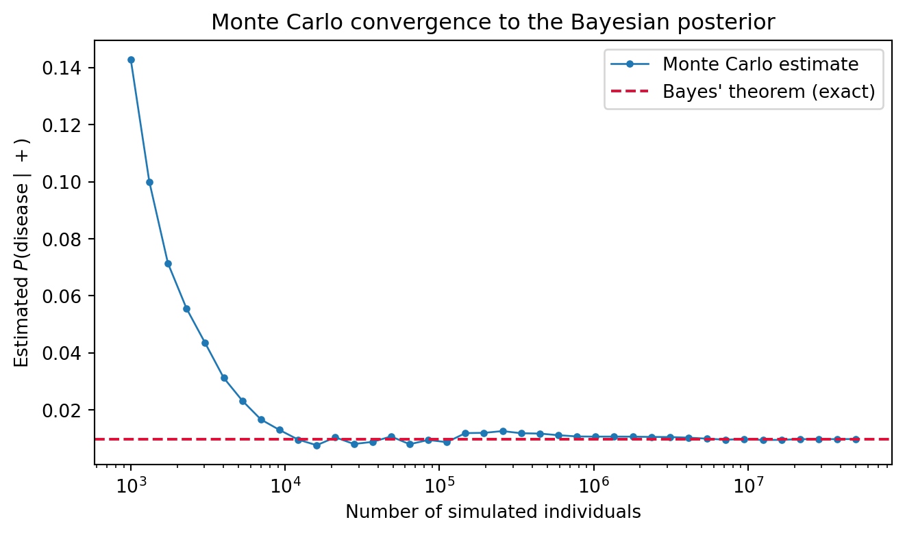
The base rate result above is the kind of claim that is easy to state and easy to doubt. A clean way to build confidence is to stop reasoning and start counting: simulate an enormous population, apply the test to each individual, and look at the empirical fraction of test positive people who are genuinely diseased. By the frequentist interpretation and the law of large numbers, that empirical conditional frequency must converge to the posterior $P(D \mid T^{+})$ that Bayes’ theorem predicts. The following self contained cell runs this Monte Carlo experiment with a fixed seed and plots the convergence.

Code

import numpy as np
import matplotlib.pyplot as plt

rng = np.random.default_rng(20260620)

# A test that is 99% accurate in both directions, for a rare disease.
prevalence  = 1.0 / 10000.0   # P(disease)
sensitivity = 0.99            # P(+ | disease)
specificity = 0.99            # P(- | no disease)

# Exact posterior P(disease | +) via the law of total probability and Bayes.
p_pos = sensitivity * prevalence + (1 - specificity) * (1 - prevalence)
posterior_exact = sensitivity * prevalence / p_pos

# Simulate a large population and apply the test to each person.
n_total = 50_000_000
has_disease = rng.random(n_total) < prevalence
test_pos = np.where(
    has_disease,
    rng.random(n_total) < sensitivity,          # diseased: true positive w.p. sensitivity
    rng.random(n_total) < (1 - specificity),    # healthy: false positive w.p. 1 - specificity
)

# Running estimate of P(disease | +) as the sample grows.
cum_pos = np.cumsum(test_pos)
cum_tp  = np.cumsum(test_pos & has_disease)
checkpoints = np.unique(np.logspace(3, np.log10(n_total), 40).astype(int))
estimates = np.array([
    cum_tp[n - 1] / cum_pos[n - 1] if cum_pos[n - 1] > 0 else np.nan
    for n in checkpoints
])

final = cum_tp[-1] / cum_pos[-1]
print(f"Exact      P(disease | +) = {posterior_exact:.6f}")
print(f"MonteCarlo P(disease | +) = {final:.6f}  (n = {n_total:,})")
print(f"Absolute error            = {abs(final - posterior_exact):.6f}")

fig, ax = plt.subplots(figsize=(7, 4.2))
ax.semilogx(checkpoints, estimates, marker="o", ms=3, lw=1, label="Monte Carlo estimate")
ax.axhline(posterior_exact, color="crimson", ls="--", label="Bayes' theorem (exact)")
ax.set_xlabel("Number of simulated individuals")
ax.set_ylabel(r"Estimated $P(\mathrm{disease} \mid +)$")
ax.set_title("Monte Carlo convergence to the Bayesian posterior")
ax.legend()
fig.tight_layout()
plt.show()

Exact      P(disease | +) = 0.009804
MonteCarlo P(disease | +) = 0.009799  (n = 50,000,000)
Absolute error            = 0.000005

The printed Monte Carlo estimate lands within a fraction of a thousandth of the exact posterior of about $0.0098$, and the curve visibly settles onto the dashed analytic line as the simulated population grows. The simulation knows nothing of Bayes’ theorem; it merely tallies outcomes. That the tally agrees with the formula is the law of large numbers turning the abstract axioms into something we can watch happen.

31.6.1 6.1 The Same Experiment in Three Languages

The logic transfers unchanged to any numerical environment. The Python panel below is the executable version run above; the Julia and Rust panels are illustrative ports that express the identical Monte Carlo estimate of the posterior.

Code

import numpy as np

rng = np.random.default_rng(20260620)
prevalence, sensitivity, specificity = 1e-4, 0.99, 0.99

n = 50_000_000
disease = rng.random(n) < prevalence
positive = np.where(disease,
                    rng.random(n) < sensitivity,
                    rng.random(n) < (1 - specificity))

posterior = np.count_nonzero(positive & disease) / np.count_nonzero(positive)
print(f"P(disease | +) ~ {posterior:.6f}")

P(disease | +) ~ 0.009799

using Random

rng = MersenneTwister(20260620)
prevalence, sensitivity, specificity = 1e-4, 0.99, 0.99

n = 50_000_000
true_pos = 0
all_pos  = 0
for _ in 1:n
    disease  = rand(rng) < prevalence
    positive = disease ? rand(rng) < sensitivity : rand(rng) < (1 - specificity)
    if positive
        all_pos += 1
        disease && (true_pos += 1)
    end
end

println("P(disease | +) ~ ", round(true_pos / all_pos, digits = 6))

// Cargo.toml: rand = "0.8"
use rand::rngs::StdRng;
use rand::{Rng, SeedableRng};

fn main() {
    let mut rng = StdRng::seed_from_u64(20260620);
    let (prevalence, sensitivity, specificity) = (1e-4_f64, 0.99_f64, 0.99_f64);

    let n: u64 = 50_000_000;
    let (mut true_pos, mut all_pos) = (0_u64, 0_u64);
    for _ in 0..n {
        let disease = rng.gen::<f64>() < prevalence;
        let positive = if disease {
            rng.gen::<f64>() < sensitivity
        } else {
            rng.gen::<f64>() < 1.0 - specificity
        };
        if positive {
            all_pos += 1;
            if disease {
                true_pos += 1;
            }
        }
    }

    println!("P(disease | +) ~ {:.6}", true_pos as f64 / all_pos as f64);
}

31.7 7. Why Probability Is the Language of Uncertainty in Machine Learning

31.7.1 7.1 Learning as Inference Under Uncertainty

Every machine learning problem is shot through with uncertainty. Training data is a finite and noisy sample drawn from a vast or infinite population. The relationship between inputs and outputs is rarely deterministic, so even a perfect model assigns probabilities rather than certainties. The parameters we estimate are themselves uncertain, known only up to the limits of what the data can reveal. And when a deployed model meets a new input, it must hazard a prediction without ever having seen that exact case before. Probability is the only mathematical framework that handles all of these uncertainties within a single coherent calculus.

This is more than a convenient metaphor. Supervised learning is typically framed as estimating a conditional distribution $P(y \mid x)$, the probability of a label given an input. A classifier that outputs a probability over classes, rather than a bare label, can express how confident it is, abstain when unsure, and be combined sensibly with other sources of information. The cross-entropy loss that trains most neural classifiers is derived directly from the principle of maximum likelihood, which seeks the parameters under which the observed data is most probable. The objective functions of deep learning, far from being arbitrary, are probabilistic statements in disguise [3].

31.7.2 7.2 Calibration, Risk, and Decisions

Because probability obeys the Kolmogorov axioms, the numbers a model produces can be checked against reality. A model is calibrated when, among all the cases it labels with probability seventy percent, roughly seventy percent indeed turn out positive. Calibration is a direct empirical test of whether a model’s stated probabilities mean what they claim, and modern deep networks are often poorly calibrated despite high accuracy, a finding that has driven a substantial line of research [5]. Without the axiomatic grounding of probability, the very notion of calibration would be meaningless.

Probability also connects learning to action. A decision maker who must choose among options weighs each by its expected outcome, the average over uncertain states weighted by their probabilities. This is where the law of total probability and conditional probability pay off operationally: they let an agent average over what it does not know to act well on average. From medical diagnosis to autonomous navigation to recommendation, deployed systems do not merely predict, they decide, and rational decision under uncertainty is built on the probabilistic foundations laid out in this chapter. A spam filter must choose whether to quarantine a message, a self-driving car must choose whether to brake, and in each case the right action depends on probabilities that the system has learned and combined according to the rules we have developed.

31.7.3 7.3 From Axioms to Systems

It is striking how far three short axioms reach. Non-negativity, normalization, and countable additivity, together with the definition of conditional probability, generate the entire apparatus that modern machine learning runs on. Bayes’ theorem, the chain rule behind autoregressive language models, the conditional independence assumptions that make graphical models tractable, the marginalization that produces evidence terms, and the maximum likelihood objectives that train neural networks all descend from this small set of starting points. When a large model assigns a probability to the next word, or a classifier reports its confidence, or a Bayesian method quantifies what it does not know, it is speaking the language whose grammar Kolmogorov fixed in 1933. Mastering that grammar is the prerequisite for everything that follows in this book.

31.8 References

Kolmogorov, A. N. Foundations of the Theory of Probability. Second English edition, Chelsea Publishing, 1956. (Translation of Grundbegriffe der Wahrscheinlichkeitsrechnung, Springer, 1933.) DOI: 10.1007/978-3-642-49888-6
Shalev-Shwartz, S. and Ben-David, S. Understanding Machine Learning: From Theory to Algorithms. Cambridge University Press, 2014. DOI: 10.1017/CBO9781107298019
Bishop, C. M. Pattern Recognition and Machine Learning. Springer, 2006. DOI: 10.1007/978-0-387-45528-0
Blei, D. M., Kucukelbir, A., and McAuliffe, J. D. “Variational Inference: A Review for Statisticians.” Journal of the American Statistical Association, vol. 112, no. 518, 2017, pp. 859 to 877. DOI: 10.1080/01621459.2017.1285773
Guo, C., Pleiss, G., Sun, Y., and Weinberger, K. Q. “On Calibration of Modern Neural Networks.” Proceedings of the 34th International Conference on Machine Learning (ICML), PMLR vol. 70, 2017, pp. 1321 to 1330. DOI: 10.5555/3305381.3305518
Çinlar, E. Probability and Stochastics. Graduate Texts in Mathematics, vol. 261, Springer, 2011. DOI: 10.1007/978-0-387-87859-1
Durrett, R. Probability: Theory and Examples. 5th edition, Cambridge University Press, 2019. DOI: 10.1017/9781108591034

# Foundations of Probability Probability is the mathematics of uncertainty. Almost every modern machine learning system, from a spam filter to a large language model, is at heart a machinery for reasoning about what is likely given what has been observed. To understand why these systems work, why they sometimes fail, and how to improve them, we need a precise account of what probability is. This chapter builds that account from the ground up. We start with the raw ingredients of a random experiment, state the axioms that any sensible notion of probability must obey, and develop the core tools of conditioning, independence, and total probability. Throughout, we connect each idea to the way uncertainty shows up in learning systems. ## 1. Sample Spaces and Events ### 1.1 The Anatomy of a Random Experiment A probabilistic model begins with an experiment whose outcome is uncertain before it is performed. The set of all possible outcomes is the **sample space**, denoted $\Omega$. Each individual outcome is an element $\omega \in \Omega$, sometimes called a sample point. The sample space is the universe of possibilities, and everything we can later say about probability is a statement about subsets of this universe. Consider a single roll of a fair die. The sample space is $\Omega = \{1, 2, 3, 4, 5, 6\}$, a finite set with six elements. If we flip a coin until the first head appears, the sample space is countably infinite, $\Omega = \{H, TH, TTH, TTTH, \ldots\}$. If we measure the time until a hard drive fails, the sample space is the continuous interval $\Omega = [0, \infty)$. These three cases, finite, countably infinite, and uncountable, require slightly different mathematical machinery, but the conceptual picture is the same. An **event** is a subset of the sample space, $A \subseteq \Omega$. We say the event $A$ occurs if the realized outcome $\omega$ belongs to $A$. For the die, the event "the roll is even" is $A = \{2, 4, 6\}$. The event "the roll is at least five" is $B = \{5, 6\}$. Events are sets, so the language of set theory becomes the language of events. The union $A \cup B$ is the event that $A$ or $B$ (or both) occur. The intersection $A \cap B$ is the event that both occur. The complement $A^c = \Omega \setminus A$ is the event that $A$ does not occur. The empty set $\varnothing$ is the impossible event, and $\Omega$ itself is the certain event. Two events are **mutually exclusive**, or disjoint, when $A \cap B = \varnothing$, meaning they cannot both occur. A collection of events is **exhaustive** when their union is all of $\Omega$. A collection that is both mutually exclusive and exhaustive forms a **partition** of the sample space, a notion we will lean on heavily when we reach the law of total probability. ### 1.2 Why We Need a Sigma-Algebra It is tempting to declare that every subset of $\Omega$ is an event to which we can assign a probability. For finite and countable sample spaces this works perfectly well. For uncountable sample spaces, such as the real line, it turns out that we cannot consistently assign probabilities to every subset without running into contradictions. The pathological sets that cause trouble are exotic and never arise in practical modeling, but their existence forces us to be careful. The resolution is to restrict attention to a collection $\mathcal{F}$ of subsets of $\Omega$ that we agree to call events. This collection must be a **sigma-algebra** (also written $\sigma$-algebra), meaning it satisfies three closure properties: 1. $\Omega \in \mathcal{F}$. 2. If $A \in \mathcal{F}$ then its complement $A^c \in \mathcal{F}$ (closure under complementation). 3. If $A_1, A_2, A_3, \ldots$ is a countable sequence of sets in $\mathcal{F}$, then their union $\bigcup_{i=1}^{\infty} A_i$ also lies in $\mathcal{F}$ (closure under countable unions). These three properties already force a great deal more. Because $\Omega \in \mathcal{F}$ and $\mathcal{F}$ is closed under complementation, the empty set $\varnothing = \Omega^c$ belongs to $\mathcal{F}$. Closure under countable unions plus De Morgan's laws gives closure under countable intersections, since $$ \bigcap_{i=1}^{\infty} A_i = \left( \bigcup_{i=1}^{\infty} A_i^c \right)^{\!c}, $$ and the right hand side is a complement of a countable union of complements, each step of which stays inside $\mathcal{F}$. Finite unions and intersections follow by padding a finite list with copies of $\varnothing$ or $\Omega$, and set differences $A \setminus B = A \cap B^c$ are covered as well. In short, any event we can construct from countably many basic events by the usual logical operations is itself a legitimate event. For a finite or countable $\Omega$ we may safely take $\mathcal{F} = 2^{\Omega}$, the power set of all subsets. For $\Omega = \mathbb{R}$ the standard choice is the **Borel sigma-algebra** $\mathcal{B}(\mathbb{R})$, the smallest sigma-algebra containing every open interval. It contains every set one meets in practice, yet it is a strict subset of the power set, which is exactly what lets a consistent probability measure exist. The triple $(\Omega, \mathcal{F}, P)$, consisting of a sample space, a sigma-algebra of events, and a probability measure $P$ defined on $\mathcal{F}$, is called a **probability space**. This is the formal object on which all of probability theory rests. In practice, machine learning practitioners rarely write down the sigma-algebra explicitly. It works quietly in the background, ensuring that quantities like expectations and conditional probabilities are well defined. But knowing it is there clarifies why probability is a theory of measure, not merely a theory of counting. ## 2. The Kolmogorov Axioms ### 2.1 Three Rules That Define Probability In 1933 Andrey Kolmogorov gave probability theory the rigorous footing it had lacked for centuries by proposing that probability is simply a measure that assigns the value one to the whole space [1]. A **probability measure** is a function $P : \mathcal{F} \to \mathbb{R}$ satisfying three axioms. The first axiom is **non-negativity**. For every event $A \in \mathcal{F}$, $$ P(A) \geq 0 . $$ Probabilities are never negative. This reflects the intuition that the chance of something cannot be less than impossible. The second axiom is **normalization**. The probability of the entire sample space is one, $$ P(\Omega) = 1 . $$ Something in $\Omega$ must happen, and we calibrate certainty to the value one. The third axiom is **countable additivity**. If $A_1, A_2, A_3, \ldots$ is a countable collection of pairwise disjoint events, meaning $A_i \cap A_j = \varnothing$ whenever $i \neq j$, then $$ P\!\left(\bigcup_{i=1}^{\infty} A_i\right) = \sum_{i=1}^{\infty} P(A_i) . $$ The probability of a union of non-overlapping events is the sum of their individual probabilities. This is the axiom that does the real work, because it lets us decompose complicated events into simpler pieces and add up the parts. That is the entire foundation. Everything else in probability, every formula and theorem, is a logical consequence of these three statements together with the structure of the probability space. ### 2.2 Consequences of the Axioms A handful of useful facts follow immediately, and it is worth seeing them proved rather than merely asserted, because every one is a short deduction from the three axioms. **Finite additivity.** Countable additivity implies the finite version. Given disjoint $A_1, \ldots, A_n$, extend the list with $A_{n+1} = A_{n+2} = \cdots = \varnothing$. These remain pairwise disjoint, and since (as shown next) $P(\varnothing) = 0$, the infinite sum collapses to the finite one, giving $P(A_1 \cup \cdots \cup A_n) = \sum_{i=1}^{n} P(A_i)$. **The empty set has probability zero.** Take $A_1 = \Omega$ and $A_i = \varnothing$ for $i \ge 2$. These are pairwise disjoint with union $\Omega$, so countable additivity gives $P(\Omega) = P(\Omega) + \sum_{i \ge 2} P(\varnothing)$. Subtracting $P(\Omega)$ leaves $\sum_{i \ge 2} P(\varnothing) = 0$, and since each term is non-negative by the first axiom, $P(\varnothing) = 0$. **The complement rule.** Because $A$ and $A^c$ are disjoint and $A \cup A^c = \Omega$, finite additivity and normalization give $P(A) + P(A^c) = P(\Omega) = 1$, hence $$ P(A^c) = 1 - P(A) . $$ **Monotonicity.** If $A \subseteq B$, then $B$ is the disjoint union of $A$ and $B \setminus A$, so $P(B) = P(A) + P(B \setminus A)$. Non-negativity of the second term yields $P(B) \ge P(A)$: larger events are at least as probable as the smaller events they contain. Applying this with $B = \Omega$ shows $P(A) \le 1$, so together with non-negativity every probability lies in $[0, 1]$. **Inclusion-exclusion for two events.** When two events may overlap, naive addition double counts the intersection. To correct for it, decompose both the union and each event into disjoint pieces. Write $$ A \cup B = (A \setminus B) \,\cup\, (A \cap B) \,\cup\, (B \setminus A), $$ a union of three pairwise disjoint sets. Finite additivity gives $P(A \cup B) = P(A \setminus B) + P(A \cap B) + P(B \setminus A)$. Separately, $A = (A \setminus B) \cup (A \cap B)$ and $B = (B \setminus A) \cup (A \cap B)$, each a disjoint split, so $P(A \setminus B) = P(A) - P(A \cap B)$ and $P(B \setminus A) = P(B) - P(A \cap B)$. Substituting these in yields the **inclusion-exclusion** principle, $$ P(A \cup B) = P(A) + P(B) - P(A \cap B) . $$ Because $P(A \cap B) \ge 0$, a direct corollary is the **union bound**, $P(A \cup B) \le P(A) + P(B)$, which extends by induction and then a limiting argument to any countable collection, $$ P\!\left(\bigcup_{i} A_i\right) \le \sum_{i} P(A_i) . $$ The union bound is one of the most heavily used tools in the theoretical analysis of machine learning. When proving that a learned model generalizes, we often need to control the probability that any one of many bad events occurs. The union bound lets us bound that combined failure probability by summing the individual failure probabilities, even when the events are dependent in complicated ways. Generalization bounds for finite hypothesis classes are built on exactly this idea [2]. ### 2.3 Interpreting What Probability Means The axioms tell us how probabilities behave but not what they signify. Two interpretations dominate. The **frequentist** view holds that the probability of an event is the long-run relative frequency with which it occurs across many independent repetitions of the experiment. The probability that a coin lands heads is the limiting fraction of heads as the number of tosses grows without bound, a statement made precise by the law of large numbers. The **Bayesian** view holds that probability is a degree of belief, a numerical measure of how confident a rational agent is in a proposition given the information available. Under this reading we may speak of the probability that a particular email is spam, or that a specific model parameter takes a certain value, even though there is no repeatable experiment in sight. Both interpretations satisfy the same Kolmogorov axioms, so the mathematics is shared even where the philosophy diverges. Machine learning draws on both: frequentist arguments justify why empirical risk minimization works, while Bayesian arguments underpin probabilistic modeling, posterior inference, and the quantification of model uncertainty. ## 3. Conditional Probability ### 3.1 Updating Beliefs in Light of Evidence The single most important operation in probabilistic reasoning is updating what we believe once we learn something. The **conditional probability** of $A$ given $B$, written $P(A \mid B)$, is the probability that $A$ occurs under the knowledge that $B$ has occurred. Provided $P(B) > 0$, it is defined by $$ P(A \mid B) = \frac{P(A \cap B)}{P(B)} . $$ The intuition is geometric. Learning that $B$ occurred shrinks the relevant universe from all of $\Omega$ down to $B$. Within this smaller universe we ask what fraction of probability mass also falls in $A$. We rescale by dividing through by $P(B)$ so that the conditional probabilities over the restricted space again sum to one. Indeed, $P(\cdot \mid B)$ is itself a perfectly valid probability measure on $\Omega$, satisfying all three Kolmogorov axioms. Return to the die. Let $A = \{$the roll is even$\} = \{2, 4, 6\}$ and $B = \{$the roll is at least four$\} = \{4, 5, 6\}$. Then $A \cap B = \{4, 6\}$, so $$ P(A \mid B) = \frac{P(\{4, 6\})}{P(\{4, 5, 6\})} = \frac{2/6}{3/6} = \frac{2}{3} . $$ Knowing the roll is at least four raises the probability that it is even from one half to two thirds, because two of the three remaining outcomes are even. ### 3.2 The Chain Rule and Bayes' Theorem Rearranging the definition gives the **multiplication rule**, $P(A \cap B) = P(A \mid B)\, P(B)$. Applied repeatedly it yields the **chain rule** for the joint probability of a sequence of events, $$ P(A_1 \cap A_2 \cap \cdots \cap A_n) = P(A_1)\, P(A_2 \mid A_1)\, P(A_3 \mid A_1 \cap A_2) \cdots P(A_n \mid A_1 \cap \cdots \cap A_{n-1}) . $$ The chain rule is the backbone of autoregressive models. A language model factorizes the probability of a sequence of tokens $w_1, \ldots, w_n$ as $P(w_1) \prod_{t=2}^{n} P(w_t \mid w_1, \ldots, w_{t-1})$, predicting each token conditioned on everything before it. Training such a model amounts to learning these conditional distributions, and generation amounts to sampling from them one step at a time. The most consequential rearrangement is **Bayes' theorem**, which inverts the direction of conditioning, $$ P(A \mid B) = \frac{P(B \mid A)\, P(A)}{P(B)} . $$ This formula lets us compute the probability of a hidden cause $A$ given an observed effect $B$ when we know the reverse relationship, the probability of the effect given the cause. In the language of inference, $P(A)$ is the **prior**, $P(B \mid A)$ is the **likelihood**, $P(B)$ is the **evidence** or marginal likelihood, and $P(A \mid B)$ is the **posterior**. Bayes' theorem is the engine of probabilistic machine learning, from naive Bayes classifiers to full Bayesian neural networks [3]. A spam filter, for instance, treats the words in a message as evidence and uses Bayes' theorem to compute the posterior probability that the message is spam given those words. ### 3.3 The Base Rate Fallacy Conditional probability is notoriously counterintuitive, and the most common error is to neglect the prior. Suppose a diagnostic test for a disease is ninety nine percent accurate in both directions, yet the disease afflicts only one person in ten thousand. If a randomly chosen person tests positive, the probability they actually have the disease is not ninety nine percent. Let us work it out exactly, because the worked example ties together every tool in this chapter. Write $D$ for the event of having the disease and $T^{+}$ for a positive test. The given quantities are the prior $P(D) = 0.0001$, the sensitivity $P(T^{+} \mid D) = 0.99$, and the specificity $P(T^{-} \mid D^c) = 0.99$, so the false positive rate is $P(T^{+} \mid D^c) = 0.01$. First compute the evidence by the law of total probability over the partition $\{D, D^c\}$, $$ P(T^{+}) = P(T^{+} \mid D)\, P(D) + P(T^{+} \mid D^c)\, P(D^c) = 0.99 \times 0.0001 + 0.01 \times 0.9999 = 0.010098 . $$ Now apply Bayes' theorem, $$ P(D \mid T^{+}) = \frac{P(T^{+} \mid D)\, P(D)}{P(T^{+})} = \frac{0.99 \times 0.0001}{0.010098} \approx 0.0098 . $$ A positive result on a ninety nine percent accurate test leaves the patient with under a one percent chance of actually being ill, because the vast pool of healthy people produces many more false positives than the tiny diseased pool produces true positives. The same arithmetic governs classifier behavior on imbalanced data. A model with excellent accuracy on each class can still produce mostly wrong positive predictions when the positive class is rare, which is why metrics like precision and recall, rooted in conditional probability, matter more than raw accuracy in such settings. ## 4. Independence ### 4.1 When Knowing One Thing Tells You Nothing About Another Two events $A$ and $B$ are **independent** when the occurrence of one carries no information about the other. Formally, $A$ and $B$ are independent if and only if $$ P(A \cap B) = P(A)\, P(B) . $$ When $P(B) > 0$, this is equivalent to the more intuitive statement $P(A \mid B) = P(A)$. Conditioning on $B$ leaves the probability of $A$ unchanged, which is exactly what we mean by saying that $B$ is uninformative about $A$. Independence is a symmetric relation, and the multiplicative definition handles the boundary cases where a conditioning probability is zero. It is worth stressing that independence is a numerical property of the probability measure, not a statement about physical or causal separation. Two events can be independent under one probability assignment and dependent under another. Independence is also easy to confuse with mutual exclusivity, but the two are nearly opposite. If $A$ and $B$ are disjoint with positive probabilities, then learning that $B$ occurred makes $A$ impossible, so they are strongly dependent rather than independent. ### 4.2 Conditional Independence and the Structure of Models A subtler and more powerful notion is **conditional independence**. Events $A$ and $B$ are conditionally independent given $C$ if $$ P(A \cap B \mid C) = P(A \mid C)\, P(B \mid C) . $$ Once we know $C$, the events $A$ and $B$ become independent, even if they were dependent without that knowledge. This is the structural assumption that makes large probabilistic models tractable. The naive Bayes classifier assumes that the features of an input are conditionally independent given the class label, which collapses an exponentially large joint distribution into a product of simple per-feature terms. Probabilistic graphical models, including Bayesian networks and Markov random fields, are essentially a calculus for expressing which conditional independences hold among many variables, and they exploit those independences to make inference and learning feasible [3]. Independence assumptions are double edged. They are what make computation possible, yet they are also where models depart most sharply from reality. The features of a real document are not truly independent given its topic, and the naive Bayes assumption is plainly false. The art of probabilistic modeling lies in choosing independence assumptions that are wrong enough to be computable but right enough to be useful. ## 5. The Law of Total Probability ### 5.1 Decomposing Uncertainty Through a Partition Often we cannot compute the probability of an event directly, but we can compute it within each of several scenarios that together cover all possibilities. The **law of total probability** assembles these pieces into a whole. Let $B_1, B_2, \ldots, B_n$ be a partition of the sample space, meaning the $B_i$ are pairwise disjoint and their union is $\Omega$, with each $P(B_i) > 0$. Then for any event $A$, $$ P(A) = \sum_{i=1}^{n} P(A \mid B_i)\, P(B_i) . $$ The derivation is short and instructive. The event $A$ can be sliced into disjoint pieces $A \cap B_i$, one for each cell of the partition, because the $B_i$ cover everything without overlap. Countable additivity gives $P(A) = \sum_i P(A \cap B_i)$, and the multiplication rule rewrites each term as $P(A \mid B_i) P(B_i)$. The result expresses the overall probability of $A$ as a weighted average of its conditional probabilities across scenarios, with the weights being the probabilities of the scenarios themselves. A quick example: suppose two factories supply a parts bin, factory one contributing sixty percent of parts with a two percent defect rate, and factory two contributing forty percent with a five percent defect rate. The probability that a randomly drawn part is defective is $0.02 \times 0.6 + 0.05 \times 0.4 = 0.032$, a clean application of the law with a two cell partition. ### 5.2 Marginalization and the Evidence Term In machine learning the law of total probability appears most often under the name **marginalization**. When we have a joint distribution over several variables and want the distribution of just one, we sum or integrate out the others. For discrete variables $X$ and $Y$, $$ P(X = x) = \sum_{y} P(X = x \mid Y = y)\, P(Y = y) = \sum_{y} P(X = x, Y = y), $$ and for continuous variables the sum becomes an integral, $p(x) = \int p(x \mid y)\, p(y)\, dy$. Marginalization is how we move from a rich joint model down to the particular quantity we care about. The law of total probability also supplies the evidence term that sits in the denominator of Bayes' theorem. Recall that the posterior is $P(A \mid B) = P(B \mid A) P(A) / P(B)$. The denominator $P(B)$ is rarely given to us directly. Instead we compute it by total probability over the partition induced by the hypothesis, $$ P(B) = \sum_{i} P(B \mid A_i)\, P(A_i), $$ which guarantees that the resulting posterior is properly normalized and sums to one across all hypotheses. In Bayesian inference this marginal likelihood is frequently the hardest quantity to evaluate, since the sum or integral may range over an enormous or continuous hypothesis space. Much of the machinery of modern Bayesian computation, from variational inference to Markov chain Monte Carlo, exists precisely to approximate this term when it cannot be computed in closed form [4]. ## 6. Verifying the Theory by Simulation The base rate result above is the kind of claim that is easy to state and easy to doubt. A clean way to build confidence is to stop reasoning and start counting: simulate an enormous population, apply the test to each individual, and look at the empirical fraction of test positive people who are genuinely diseased. By the frequentist interpretation and the law of large numbers, that empirical conditional frequency must converge to the posterior $P(D \mid T^{+})$ that Bayes' theorem predicts. The following self contained cell runs this Monte Carlo experiment with a fixed seed and plots the convergence. ```{python} import numpy as np import matplotlib.pyplot as plt rng = np.random.default_rng(20260620) # A test that is 99% accurate in both directions, for a rare disease. prevalence = 1.0 / 10000.0 # P(disease) sensitivity = 0.99 # P(+ | disease) specificity = 0.99 # P(- | no disease) # Exact posterior P(disease | +) via the law of total probability and Bayes. p_pos = sensitivity * prevalence + (1 - specificity) * (1 - prevalence) posterior_exact = sensitivity * prevalence / p_pos # Simulate a large population and apply the test to each person. n_total = 50_000_000 has_disease = rng.random(n_total) < prevalence test_pos = np.where( has_disease, rng.random(n_total) < sensitivity, # diseased: true positive w.p. sensitivity rng.random(n_total) < (1 - specificity), # healthy: false positive w.p. 1 - specificity ) # Running estimate of P(disease | +) as the sample grows. cum_pos = np.cumsum(test_pos) cum_tp = np.cumsum(test_pos & has_disease) checkpoints = np.unique(np.logspace(3, np.log10(n_total), 40).astype(int)) estimates = np.array([ cum_tp[n - 1] / cum_pos[n - 1] if cum_pos[n - 1] > 0 else np.nan for n in checkpoints ]) final = cum_tp[-1] / cum_pos[-1] print(f"Exact P(disease | +) = {posterior_exact:.6f}") print(f"MonteCarlo P(disease | +) = {final:.6f} (n = {n_total:,})") print(f"Absolute error = {abs(final - posterior_exact):.6f}") fig, ax = plt.subplots(figsize=(7, 4.2)) ax.semilogx(checkpoints, estimates, marker="o", ms=3, lw=1, label="Monte Carlo estimate") ax.axhline(posterior_exact, color="crimson", ls="--", label="Bayes' theorem (exact)") ax.set_xlabel("Number of simulated individuals") ax.set_ylabel(r"Estimated $P(\mathrm{disease} \mid +)$") ax.set_title("Monte Carlo convergence to the Bayesian posterior") ax.legend() fig.tight_layout() plt.show() ``` The printed Monte Carlo estimate lands within a fraction of a thousandth of the exact posterior of about $0.0098$, and the curve visibly settles onto the dashed analytic line as the simulated population grows. The simulation knows nothing of Bayes' theorem; it merely tallies outcomes. That the tally agrees with the formula is the law of large numbers turning the abstract axioms into something we can watch happen. ### 6.1 The Same Experiment in Three Languages The logic transfers unchanged to any numerical environment. The Python panel below is the executable version run above; the Julia and Rust panels are illustrative ports that express the identical Monte Carlo estimate of the posterior. ::: {.panel-tabset} ## Python ```{python} import numpy as np rng = np.random.default_rng(20260620) prevalence, sensitivity, specificity = 1e-4, 0.99, 0.99 n = 50_000_000 disease = rng.random(n) < prevalence positive = np.where(disease, rng.random(n) < sensitivity, rng.random(n) < (1 - specificity)) posterior = np.count_nonzero(positive & disease) / np.count_nonzero(positive) print(f"P(disease | +) ~ {posterior:.6f}") ``` ## Julia ```julia using Random rng = MersenneTwister(20260620) prevalence, sensitivity, specificity = 1e-4, 0.99, 0.99 n = 50_000_000 true_pos = 0 all_pos = 0 for _ in 1:n disease = rand(rng) < prevalence positive = disease ? rand(rng) < sensitivity : rand(rng) < (1 - specificity) if positive all_pos += 1 disease && (true_pos += 1) end end println("P(disease | +) ~ ", round(true_pos / all_pos, digits = 6)) ``` ## Rust ```rust // Cargo.toml: rand = "0.8" use rand::rngs::StdRng; use rand::{Rng, SeedableRng}; fn main() { let mut rng = StdRng::seed_from_u64(20260620); let (prevalence, sensitivity, specificity) = (1e-4_f64, 0.99_f64, 0.99_f64); let n: u64 = 50_000_000; let (mut true_pos, mut all_pos) = (0_u64, 0_u64); for _ in 0..n { let disease = rng.gen::<f64>() < prevalence; let positive = if disease { rng.gen::<f64>() < sensitivity } else { rng.gen::<f64>() < 1.0 - specificity }; if positive { all_pos += 1; if disease { true_pos += 1; } } } println!("P(disease | +) ~ {:.6}", true_pos as f64 / all_pos as f64); } ``` ::: ## 7. Why Probability Is the Language of Uncertainty in Machine Learning ### 7.1 Learning as Inference Under Uncertainty Every machine learning problem is shot through with uncertainty. Training data is a finite and noisy sample drawn from a vast or infinite population. The relationship between inputs and outputs is rarely deterministic, so even a perfect model assigns probabilities rather than certainties. The parameters we estimate are themselves uncertain, known only up to the limits of what the data can reveal. And when a deployed model meets a new input, it must hazard a prediction without ever having seen that exact case before. Probability is the only mathematical framework that handles all of these uncertainties within a single coherent calculus. This is more than a convenient metaphor. Supervised learning is typically framed as estimating a conditional distribution $P(y \mid x)$, the probability of a label given an input. A classifier that outputs a probability over classes, rather than a bare label, can express how confident it is, abstain when unsure, and be combined sensibly with other sources of information. The cross-entropy loss that trains most neural classifiers is derived directly from the principle of maximum likelihood, which seeks the parameters under which the observed data is most probable. The objective functions of deep learning, far from being arbitrary, are probabilistic statements in disguise [3]. ### 7.2 Calibration, Risk, and Decisions Because probability obeys the Kolmogorov axioms, the numbers a model produces can be checked against reality. A model is **calibrated** when, among all the cases it labels with probability seventy percent, roughly seventy percent indeed turn out positive. Calibration is a direct empirical test of whether a model's stated probabilities mean what they claim, and modern deep networks are often poorly calibrated despite high accuracy, a finding that has driven a substantial line of research [5]. Without the axiomatic grounding of probability, the very notion of calibration would be meaningless. Probability also connects learning to action. A decision maker who must choose among options weighs each by its expected outcome, the average over uncertain states weighted by their probabilities. This is where the law of total probability and conditional probability pay off operationally: they let an agent average over what it does not know to act well on average. From medical diagnosis to autonomous navigation to recommendation, deployed systems do not merely predict, they decide, and rational decision under uncertainty is built on the probabilistic foundations laid out in this chapter. A spam filter must choose whether to quarantine a message, a self-driving car must choose whether to brake, and in each case the right action depends on probabilities that the system has learned and combined according to the rules we have developed. ### 7.3 From Axioms to Systems It is striking how far three short axioms reach. Non-negativity, normalization, and countable additivity, together with the definition of conditional probability, generate the entire apparatus that modern machine learning runs on. Bayes' theorem, the chain rule behind autoregressive language models, the conditional independence assumptions that make graphical models tractable, the marginalization that produces evidence terms, and the maximum likelihood objectives that train neural networks all descend from this small set of starting points. When a large model assigns a probability to the next word, or a classifier reports its confidence, or a Bayesian method quantifies what it does not know, it is speaking the language whose grammar Kolmogorov fixed in 1933. Mastering that grammar is the prerequisite for everything that follows in this book. ## References 1. Kolmogorov, A. N. *Foundations of the Theory of Probability*. Second English edition, Chelsea Publishing, 1956. (Translation of *Grundbegriffe der Wahrscheinlichkeitsrechnung*, Springer, 1933.) DOI: [10.1007/978-3-642-49888-6](https://doi.org/10.1007/978-3-642-49888-6) 2. Shalev-Shwartz, S. and Ben-David, S. *Understanding Machine Learning: From Theory to Algorithms*. Cambridge University Press, 2014. DOI: [10.1017/CBO9781107298019](https://doi.org/10.1017/CBO9781107298019) 3. Bishop, C. M. *Pattern Recognition and Machine Learning*. Springer, 2006. DOI: [10.1007/978-0-387-45528-0](https://doi.org/10.1007/978-0-387-45528-0) 4. Blei, D. M., Kucukelbir, A., and McAuliffe, J. D. "Variational Inference: A Review for Statisticians." *Journal of the American Statistical Association*, vol. 112, no. 518, 2017, pp. 859 to 877. DOI: [10.1080/01621459.2017.1285773](https://doi.org/10.1080/01621459.2017.1285773) 5. Guo, C., Pleiss, G., Sun, Y., and Weinberger, K. Q. "On Calibration of Modern Neural Networks." *Proceedings of the 34th International Conference on Machine Learning (ICML)*, PMLR vol. 70, 2017, pp. 1321 to 1330. DOI: [10.5555/3305381.3305518](https://doi.org/10.5555/3305381.3305518) 6. Çinlar, E. *Probability and Stochastics*. Graduate Texts in Mathematics, vol. 261, Springer, 2011. DOI: [10.1007/978-0-387-87859-1](https://doi.org/10.1007/978-0-387-87859-1) 7. Durrett, R. *Probability: Theory and Examples*. 5th edition, Cambridge University Press, 2019. DOI: [10.1017/9781108591034](https://doi.org/10.1017/9781108591034)