Probability gives machine learning its language for reasoning under uncertainty, and Bayes theorem is the engine that turns observations into updated belief. This chapter develops the theorem from first principles, introduces priors, likelihoods, and posteriors, contrasts maximum likelihood with maximum a posteriori estimation, works through a conjugate prior example in full, and closes with the Bayesian view of learning as the accumulation of evidence. Throughout, the goal is to show how these ideas live inside the models that practitioners build every day.
35.1 1. From Conditional Probability to Bayes Theorem
35.1.1 1.1 Conditional probability and the product rule
The starting point is conditional probability. For two events \(A\) and \(B\) with \(P(B) > 0\), the probability of \(A\) given that \(B\) has occurred is
\[
P(A \mid B) = \frac{P(A \cap B)}{P(B)}.
\]
This definition says that once we know \(B\) holds, the relevant universe shrinks to the outcomes consistent with \(B\), and we renormalize accordingly. Rearranging gives the product rule, \(P(A \cap B) = P(A \mid B)\,P(B)\). By symmetry we also have \(P(A \cap B) = P(B \mid A)\,P(A)\). Setting these two expressions equal produces the kernel of everything that follows:
\[
P(A \mid B)\,P(B) = P(B \mid A)\,P(A).
\]
35.1.2 1.2 The theorem itself
Dividing through by \(P(B)\) yields Bayes theorem in its most familiar form:
\[
P(A \mid B) = \frac{P(B \mid A)\,P(A)}{P(B)}.
\]
The result was published posthumously in 1763 from the work of Thomas Bayes, and was independently developed and generalized by Pierre Simon Laplace [1]. The formula looks almost trivial as algebra, yet its interpretive force is large. It tells us how to invert a conditional. We often know \(P(\text{evidence} \mid \text{hypothesis})\), the probability of seeing data if some hypothesis were true, but what we actually want is \(P(\text{hypothesis} \mid \text{evidence})\), the credibility of the hypothesis after seeing the data. Bayes theorem is the bridge between the two.
35.1.3 1.3 The denominator and the law of total probability
The denominator \(P(B)\) is the probability of the evidence under all hypotheses considered. When the hypotheses form a partition \(\{A_1, A_2, \dots, A_k\}\) of the sample space, the law of total probability expands it:
This term, often called the marginal likelihood or the evidence, acts as a normalizing constant. It guarantees that the posterior probabilities across hypotheses sum to one. In many practical settings the marginal likelihood is the hardest piece to compute, and much of modern Bayesian computation, from Markov chain Monte Carlo to variational inference, exists precisely to sidestep or approximate it.
35.1.4 1.4 A concrete illustration
Consider a diagnostic test for a condition present in 1 percent of a population. The test detects the condition correctly 99 percent of the time, \(P(+ \mid D) = 0.99\), and produces a false positive 5 percent of the time, \(P(+ \mid \neg D) = 0.05\). A patient tests positive. What is the probability they have the condition? The prior is \(P(D) = 0.01\). The evidence is
Despite an accurate test, the probability of disease given a positive result is only about 17 percent, because the condition is rare. This base rate effect is one of the most consequential lessons of Bayesian reasoning, and it explains why classifiers trained on imbalanced data can mislead anyone who ignores the prior.
35.2 2. Priors, Likelihoods, and Posteriors
35.2.1 2.1 The parametric setup
In machine learning we rarely reason about a single event. Instead we reason about a parameter \(\theta\) that indexes a family of models, given observed data \(\mathcal{D}\). Bayes theorem then reads
Each piece has a name and a role. The term \(p(\theta)\) is the prior, encoding what we believe about \(\theta\) before seeing any data. The term \(p(\mathcal{D} \mid \theta)\) is the likelihood, viewed as a function of \(\theta\) for fixed data, measuring how well each parameter value explains what we observed. The term \(p(\theta \mid \mathcal{D})\) is the posterior, our updated belief after the data has been folded in. The denominator \(p(\mathcal{D}) = \int p(\mathcal{D} \mid \theta)\,p(\theta)\,d\theta\) is the marginal likelihood.
A useful shorthand captures the proportional structure:
The posterior is proportional to likelihood times prior, with the marginal likelihood supplying only the constant that makes it integrate to one. For many tasks, such as finding the most probable parameter or sampling from the posterior, the constant is irrelevant, which is why so much of Bayesian practice works with unnormalized densities.
35.2.2 2.2 The likelihood as a function, not a probability
A subtle but important point is that the likelihood is not a probability distribution over \(\theta\). When we write \(p(\mathcal{D} \mid \theta)\) and hold \(\mathcal{D}\) fixed while varying \(\theta\), the function does not integrate to one over \(\theta\) and need not even be bounded in a way that suggests probability. It is a function that scores parameter values by the plausibility they assign to the data. This distinction, articulated by R. A. Fisher [2], is what separates frequentist likelihood reasoning from the Bayesian act of placing a distribution on \(\theta\) through the prior.
35.2.3 2.3 Choosing priors
The prior is where Bayesian inference invites both its greatest power and its sharpest criticism. A prior can encode genuine domain knowledge, for example that a click through rate is small or that a regression coefficient is near zero. Priors fall loosely into categories. An informative prior carries substantive belief. A weakly informative prior gently constrains the parameter to plausible ranges without dominating the data. A noninformative or reference prior aims to let the data speak, though truly objective priors are harder to define than they first appear. Regularization in machine learning is, as we will see, a prior in disguise, so the choice of prior is not an exotic ritual but a routine modeling decision that practitioners already make.
35.2.4 2.4 The posterior as the object of interest
The posterior is the complete answer that Bayesian inference provides. It is not a single number but a distribution, and from it we can extract whatever summary a task requires. The posterior mean gives a point estimate that minimizes expected squared error. The posterior mode gives the most probable value. Credible intervals, regions containing a stated fraction of posterior mass, quantify uncertainty in a way that the frequentist confidence interval does not, since a 95 percent credible interval genuinely contains the parameter with probability 0.95 under the model. Predictions about new data come from the posterior predictive distribution,
which averages over all parameter values weighted by their posterior plausibility rather than committing to one estimate. This averaging is what gives Bayesian predictions their characteristic robustness to overfitting.
35.3 3. Maximum Likelihood and Maximum a Posteriori Estimation
35.3.1 3.1 Maximum likelihood estimation
Often we want a single best parameter rather than a full distribution. Maximum likelihood estimation, or MLE, chooses the parameter that makes the observed data most probable:
Because products of probabilities underflow and are awkward to differentiate, we usually maximize the log likelihood instead. For independent and identically distributed data \(\mathcal{D} = \{x_1, \dots, x_n\}\),
MLE is the workhorse behind much of classical statistics and a great deal of deep learning. Training a neural network classifier by minimizing cross entropy loss is exactly maximum likelihood estimation under a categorical likelihood, and fitting a regression by minimizing squared error is maximum likelihood under a Gaussian noise model. The estimator has attractive asymptotic properties, including consistency and efficiency, but with limited data it can overfit, since it cares only about fitting the sample and carries no preference for simpler or more plausible parameters.
35.3.2 3.2 Maximum a posteriori estimation
Maximum a posteriori estimation, or MAP, instead maximizes the posterior:
MAP is MLE plus a term that pulls the estimate toward regions favored by the prior. When the prior is flat, the second term is constant and MAP reduces to MLE. As the data grows, the log likelihood scales with \(n\) while the log prior stays fixed, so the prior is steadily overwhelmed and MAP converges toward MLE. The prior matters most when data is scarce, which is precisely when extra structure is most valuable.
35.3.3 3.3 Regularization is a MAP estimate
The connection between MAP and regularization is one of the most clarifying ideas in machine learning. Consider linear regression with Gaussian likelihood and a zero mean Gaussian prior on the weights, \(p(w) = \mathcal{N}(0, \tau^2 I)\). The log prior contributes a term proportional to \(-\frac{1}{2\tau^2}\lVert w \rVert_2^2\). Maximizing the log posterior is therefore equivalent to minimizing squared error plus an \(L_2\) penalty on the weights, which is exactly ridge regression. The regularization strength \(\lambda\) corresponds to the ratio of noise variance to prior variance, so a tighter prior means stronger regularization. If we instead place a Laplace prior on the weights, the log prior contributes an \(L_1\) penalty, recovering the lasso. What looks in one community like a tuning trick to prevent overfitting is, from the Bayesian side, simply the influence of a prior belief that weights should be small.
35.3.4 3.4 MLE and MAP side by side on the Bernoulli model
The beta binomial setting makes the MLE versus MAP comparison fully concrete. With \(k\) successes in \(n\) Bernoulli trials, the log likelihood is
the familiar sample proportion. For MAP we add the log of a \(\text{Beta}(\alpha, \beta)\) prior, \(\log p(\theta) = (\alpha - 1)\log \theta + (\beta - 1)\log(1 - \theta) - \log B(\alpha, \beta)\). The constant drops under differentiation, so the objective becomes
which has exactly the form of the log likelihood with \(k \mapsto k + \alpha - 1\) and \(n - k \mapsto n - k + \beta - 1\). Reusing the MLE calculation gives
the mode of the posterior \(\text{Beta}(\alpha + k, \beta + n - k)\). The prior acts as \(\alpha - 1\) pseudo successes and \(\beta - 1\) pseudo failures padded onto the data. As \(n \to \infty\) the pseudo counts become negligible and \(\hat{\theta}_{\text{MAP}} \to \hat{\theta}_{\text{MLE}}\), the formal statement of the earlier claim that data eventually overwhelms the prior.
35.3.5 3.5 What MAP loses
MAP gives a point and therefore discards the uncertainty that the full posterior carries. It also has a less obvious flaw: it is not invariant to reparameterization. Because the mode of a density changes under a nonlinear change of variables in a way the mean does not, the MAP estimate can shift if we rescale or transform the parameter, even though the underlying belief is unchanged. The posterior mean and the full posterior do not suffer this defect. For tasks where calibrated uncertainty matters, such as active learning, Bayesian optimization, or risk sensitive decision making, the full posterior is worth the additional computational cost that point estimates avoid.
35.4 4. Conjugate Priors: A Worked Example
35.4.1 4.1 The idea of conjugacy
Computing a posterior generally requires the troublesome marginal likelihood integral. Conjugate priors offer an elegant escape. A prior is conjugate to a likelihood when the resulting posterior belongs to the same family as the prior. The data then updates the parameters of that family in closed form, with no integration required. Conjugate pairs are limited in scope, but they are exact, fast, and pedagogically transparent, which is why they anchor any first treatment of Bayesian inference [3, 4].
35.4.2 4.2 The beta binomial model
The cleanest example is the Beta prior with a Bernoulli or binomial likelihood, a model for estimating an unknown probability \(\theta \in [0, 1]\), such as the success rate of a treatment or the conversion rate of a web page. The Beta distribution has density
where \(\alpha > 0\) and \(\beta > 0\) are shape parameters and \(B(\alpha, \beta)\) is the Beta function that normalizes the density. The parameters \(\alpha\) and \(\beta\) behave like counts of prior successes and failures, so \(\text{Beta}(1, 1)\) is the uniform prior expressing complete ignorance, while \(\text{Beta}(20, 20)\) expresses a confident prior belief that \(\theta\) is near one half.
Suppose we observe \(n\) independent Bernoulli trials with \(k\) successes. The likelihood is
No integral was evaluated. The update rule is simply to add the observed successes to \(\alpha\) and the observed failures to \(\beta\). This is conjugacy at work, and it makes the prior parameters interpretable as pseudo counts, fictional observations we bring to the problem before the real data arrives.
To see that the result is exact rather than merely proportional, restore the normalizing constants. The joint numerator is
The marginal likelihood is the integral of this over \(\theta\), and the Beta function is defined precisely so that \(\int_0^1 \theta^{a - 1}(1 - \theta)^{b - 1}\,d\theta = B(a, b)\). Hence
confirming that the posterior is a properly normalized Beta density with the updated parameters.
35.4.4 4.4 A numerical pass
Suppose a prior of \(\text{Beta}(2, 2)\), a mild belief centered at one half, and we observe 8 successes in 10 trials. The posterior is \(\text{Beta}(2 + 8, \; 2 + 2) = \text{Beta}(10, 4)\). The posterior mean of a \(\text{Beta}(\alpha, \beta)\) is \(\alpha / (\alpha + \beta)\), so our estimate of \(\theta\) is
This sits between the prior mean of 0.5 and the raw data proportion of 0.8, a compromise weighted by how much evidence each side carries. The MAP estimate, the mode of the Beta, is \((\alpha - 1)/(\alpha + \beta - 2) = 9/12 = 0.75\), while the MLE that ignores the prior would be \(8/10 = 0.8\). The three estimates differ visibly here because the data set is small, and they would converge as the number of trials grew. We can also report a 95 percent credible interval by reading off the appropriate quantiles of \(\text{Beta}(10, 4)\), giving an honest sense of how uncertain the estimate remains.
35.4.5 4.5 Other conjugate pairs and their reach
The beta binomial pair is one of a small family of conjugate relationships. The Gaussian likelihood with known variance has a Gaussian conjugate prior on the mean. The Poisson likelihood pairs with a Gamma prior on the rate. The categorical and multinomial likelihoods pair with the Dirichlet prior, a generalization of the Beta to more than two outcomes that underlies models such as latent Dirichlet allocation for topic modeling and the smoothing of naive Bayes text classifiers. These conjugate forms recur across applied machine learning, from Thompson sampling in multi armed bandits, where a Beta posterior over each arm drives exploration, to the closed form updates inside many probabilistic graphical models. Real problems often break conjugacy, which forces the approximate methods mentioned earlier, but the conjugate cases remain the conceptual reference point because they show exactly what updating belief looks like when it can be done in closed form.
35.4.6 4.6 Watching the posterior update in code
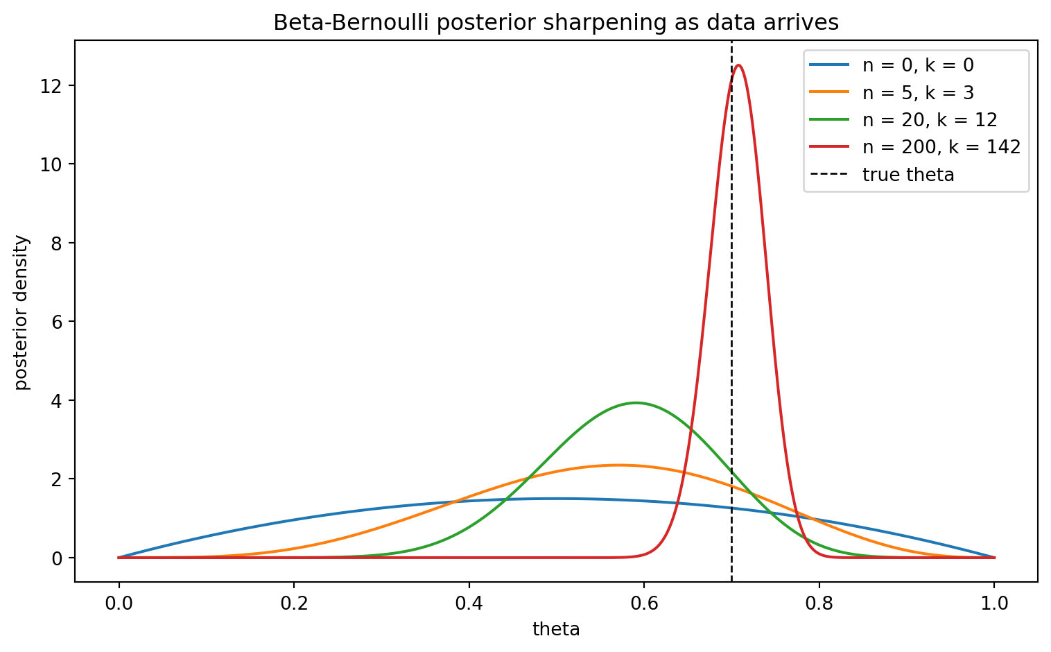
The closed form update lets us watch belief sharpen as data arrives without any sampling or integration. The cell below starts from a \(\text{Beta}(2, 2)\) prior, streams in Bernoulli trials from a coin with true bias \(0.7\), and reports the posterior mean, MAP estimate, and a 95 percent credible interval at several sample sizes. Because the update is conjugate, each snapshot is just an arithmetic adjustment of the shape parameters.
Code
import numpy as npimport matplotlib.pyplot as pltfrom scipy.stats import beta as beta_distrng = np.random.default_rng(42)theta_true =0.7# the bias we are trying to recoveralpha0, beta0 =2.0, 2.0# mild prior centered at one halfn_total =200data = rng.binomial(1, theta_true, size=n_total)snapshots = [0, 5, 20, 200]theta_grid = np.linspace(0, 1, 500)fig, ax = plt.subplots(figsize=(8, 5))print("n successes post_mean MAP 95% credible interval")for n in snapshots: k =int(data[:n].sum()) a_post = alpha0 + k # add successes to alpha b_post = beta0 + (n - k) # add failures to beta post = beta_dist(a_post, b_post) post_mean = a_post / (a_post + b_post) post_mode = (a_post -1) / (a_post + b_post -2) if a_post >1and b_post >1elsefloat("nan") lo, hi = post.ppf(0.025), post.ppf(0.975)print(f"{n:<5d}{k:<11d}{post_mean:<11.4f}{post_mode:<8.4f}[{lo:.4f}, {hi:.4f}]") ax.plot(theta_grid, post.pdf(theta_grid), label=f"n = {n}, k = {k}")ax.axvline(theta_true, color="black", linestyle="--", linewidth=1, label="true theta")ax.set_xlabel("theta")ax.set_ylabel("posterior density")ax.set_title("Beta-Bernoulli posterior sharpening as data arrives")ax.legend()fig.tight_layout()plt.show()
The printed table shows the posterior mean drifting from the prior value of \(0.5\) toward the true bias as evidence accumulates, while the credible interval narrows from a wide band to a tight one. The plotted densities tell the same story visually: each curve is sharper and more centered on \(0.7\) than the last.
35.4.7 4.7 The same update in three languages
The conjugate update is so simple that it reads almost identically across languages. The Python version is executed above; the Julia and Rust versions below are illustrative, computing the posterior parameters and mean for a single batch of \(k\) successes in \(n\) trials.
The deepest contribution of Bayesian thinking is its account of what learning is. Learning is the revision of belief in light of evidence, carried out by the mechanical application of Bayes theorem. The posterior from today becomes the prior for tomorrow. Given a first batch of data \(\mathcal{D}_1\) and then a second batch \(\mathcal{D}_2\), the posterior after both, assuming the batches are conditionally independent given \(\theta\), factors as
The posterior after the first batch plays the role of prior for the second. This recursive structure means that Bayesian learning is naturally sequential and online: belief can be updated one observation at a time, and the order of independent observations does not matter. It is a formal model of how a rational agent should accumulate knowledge, and it provides a coherent foundation for continual learning systems that must adapt as data streams in.
35.5.2 5.2 Marginalization and Occam’s razor
A striking feature of the Bayesian framework is that it penalizes unnecessary complexity automatically. When we compare models by their marginal likelihood \(p(\mathcal{D} \mid \mathcal{M})\), a model that spreads its predictive mass thinly across many possible data sets is penalized relative to one that concentrates mass on the data actually observed. A model too simple cannot fit the data, while a model too flexible dilutes its predictions over outcomes that never occurred. The marginal likelihood favors the model that strikes the balance, an effect often called the Bayesian Occam’s razor [5]. This emerges from integrating over parameters rather than fitting them, and it requires no separate complexity penalty bolted on by hand. The same machinery that updates parameters also adjudicates between competing model structures.
35.5.3 5.3 Bayesian methods in modern machine learning
Although exact Bayesian inference is intractable for large models, its influence is pervasive. Bayesian linear regression and Gaussian processes provide closed form or near closed form posteriors that deliver calibrated uncertainty, valuable in Bayesian optimization for tuning expensive systems. Approximate inference methods, including variational inference and Markov chain Monte Carlo, make Bayesian treatment feasible for richer models, and variational inference in particular connects to the training of variational autoencoders [6]. Bayesian neural networks place distributions over weights to capture model uncertainty, and even practical heuristics such as dropout at test time and deep ensembles can be read as crude approximations to posterior averaging. The recurring theme is that representing uncertainty, rather than collapsing to a single answer, makes systems more honest about what they do not know, which matters wherever a model informs a consequential decision.
35.5.4 5.4 Frequentist and Bayesian perspectives in practice
It would be a mistake to treat the Bayesian and frequentist views as warring camps that a practitioner must choose between. The two perspectives illuminate the same models from different angles. MLE and MAP are point estimates that often suffice and scale beautifully, and the cross entropy and squared error losses that dominate deep learning are likelihood based at heart. When data is plentiful, priors wash out and the two schools largely agree. The Bayesian apparatus earns its cost precisely when data is scarce, when prior knowledge is genuine and worth encoding, or when downstream decisions demand calibrated uncertainty rather than a bare prediction. A mature practitioner reaches for the framework that fits the problem, and understands that regularization, smoothing, and ensembling are already Bayesian ideas wearing everyday clothes. Seen this way, Bayes theorem is not a niche technique but a unifying lens on the act of learning from data.
35.6 References
Bayes, T. and Price, R. (1763). An Essay towards solving a Problem in the Doctrine of Chances. Philosophical Transactions of the Royal Society of London, 53, 370 to 418. https://doi.org/10.1098/rstl.1763.0053
Fisher, R. A. (1922). On the Mathematical Foundations of Theoretical Statistics. Philosophical Transactions of the Royal Society A, 222, 309 to 368. https://doi.org/10.1098/rsta.1922.0009
Gelman, A., Carlin, J. B., Stern, H. S., Dunson, D. B., Vehtari, A., and Rubin, D. B. (2013). Bayesian Data Analysis, 3rd edition. Chapman and Hall/CRC. https://doi.org/10.1201/b16018
Diaconis, P. and Ylvisaker, D. (1979). Conjugate Priors for Exponential Families. Annals of Statistics, 7(2), 269 to 281. https://doi.org/10.1214/aos/1176344611
MacKay, D. J. C. (1992). Bayesian Interpolation. Neural Computation, 4(3), 415 to 447. https://doi.org/10.1162/neco.1992.4.3.415
Kingma, D. P. and Welling, M. (2019). An Introduction to Variational Autoencoders. Foundations and Trends in Machine Learning, 12(4), 307 to 392. https://doi.org/10.1561/2200000056
Bishop, C. M. (2006). Pattern Recognition and Machine Learning. Springer. https://link.springer.com/book/9780387310732
Murphy, K. P. (2022). Probabilistic Machine Learning: An Introduction. MIT Press. https://probml.github.io/pml-book/book1.html
Source Code
# Bayes Theorem and Bayesian InferenceProbability gives machine learning its language for reasoning under uncertainty, and Bayes theorem is the engine that turns observations into updated belief. This chapter develops the theorem from first principles, introduces priors, likelihoods, and posteriors, contrasts maximum likelihood with maximum a posteriori estimation, works through a conjugate prior example in full, and closes with the Bayesian view of learning as the accumulation of evidence. Throughout, the goal is to show how these ideas live inside the models that practitioners build every day.## 1. From Conditional Probability to Bayes Theorem### 1.1 Conditional probability and the product ruleThe starting point is conditional probability. For two events $A$ and $B$ with $P(B) > 0$, the probability of $A$ given that $B$ has occurred is$$P(A \mid B) = \frac{P(A \cap B)}{P(B)}.$$This definition says that once we know $B$ holds, the relevant universe shrinks to the outcomes consistent with $B$, and we renormalize accordingly. Rearranging gives the product rule, $P(A \cap B) = P(A \mid B)\,P(B)$. By symmetry we also have $P(A \cap B) = P(B \mid A)\,P(A)$. Setting these two expressions equal produces the kernel of everything that follows:$$P(A \mid B)\,P(B) = P(B \mid A)\,P(A).$$### 1.2 The theorem itselfDividing through by $P(B)$ yields Bayes theorem in its most familiar form:$$P(A \mid B) = \frac{P(B \mid A)\,P(A)}{P(B)}.$$The result was published posthumously in 1763 from the work of Thomas Bayes, and was independently developed and generalized by Pierre Simon Laplace [1]. The formula looks almost trivial as algebra, yet its interpretive force is large. It tells us how to invert a conditional. We often know $P(\text{evidence} \mid \text{hypothesis})$, the probability of seeing data if some hypothesis were true, but what we actually want is $P(\text{hypothesis} \mid \text{evidence})$, the credibility of the hypothesis after seeing the data. Bayes theorem is the bridge between the two.### 1.3 The denominator and the law of total probabilityThe denominator $P(B)$ is the probability of the evidence under all hypotheses considered. When the hypotheses form a partition $\{A_1, A_2, \dots, A_k\}$ of the sample space, the law of total probability expands it:$$P(B) = \sum_{i=1}^{k} P(B \mid A_i)\,P(A_i).$$This term, often called the marginal likelihood or the evidence, acts as a normalizing constant. It guarantees that the posterior probabilities across hypotheses sum to one. In many practical settings the marginal likelihood is the hardest piece to compute, and much of modern Bayesian computation, from Markov chain Monte Carlo to variational inference, exists precisely to sidestep or approximate it.### 1.4 A concrete illustrationConsider a diagnostic test for a condition present in 1 percent of a population. The test detects the condition correctly 99 percent of the time, $P(+ \mid D) = 0.99$, and produces a false positive 5 percent of the time, $P(+ \mid \neg D) = 0.05$. A patient tests positive. What is the probability they have the condition? The prior is $P(D) = 0.01$. The evidence is$$P(+) = P(+ \mid D)P(D) + P(+ \mid \neg D)P(\neg D) = 0.99 \cdot 0.01 + 0.05 \cdot 0.99 = 0.0594.$$The posterior is then$$P(D \mid +) = \frac{0.99 \cdot 0.01}{0.0594} \approx 0.167.$$Despite an accurate test, the probability of disease given a positive result is only about 17 percent, because the condition is rare. This base rate effect is one of the most consequential lessons of Bayesian reasoning, and it explains why classifiers trained on imbalanced data can mislead anyone who ignores the prior.## 2. Priors, Likelihoods, and Posteriors### 2.1 The parametric setupIn machine learning we rarely reason about a single event. Instead we reason about a parameter $\theta$ that indexes a family of models, given observed data $\mathcal{D}$. Bayes theorem then reads$$p(\theta \mid \mathcal{D}) = \frac{p(\mathcal{D} \mid \theta)\,p(\theta)}{p(\mathcal{D})}.$$Each piece has a name and a role. The term $p(\theta)$ is the prior, encoding what we believe about $\theta$ before seeing any data. The term $p(\mathcal{D} \mid \theta)$ is the likelihood, viewed as a function of $\theta$ for fixed data, measuring how well each parameter value explains what we observed. The term $p(\theta \mid \mathcal{D})$ is the posterior, our updated belief after the data has been folded in. The denominator $p(\mathcal{D}) = \int p(\mathcal{D} \mid \theta)\,p(\theta)\,d\theta$ is the marginal likelihood.A useful shorthand captures the proportional structure:$$\underbrace{p(\theta \mid \mathcal{D})}_{\text{posterior}} \;\propto\; \underbrace{p(\mathcal{D} \mid \theta)}_{\text{likelihood}} \;\cdot\; \underbrace{p(\theta)}_{\text{prior}}.$$The posterior is proportional to likelihood times prior, with the marginal likelihood supplying only the constant that makes it integrate to one. For many tasks, such as finding the most probable parameter or sampling from the posterior, the constant is irrelevant, which is why so much of Bayesian practice works with unnormalized densities.### 2.2 The likelihood as a function, not a probabilityA subtle but important point is that the likelihood is not a probability distribution over $\theta$. When we write $p(\mathcal{D} \mid \theta)$ and hold $\mathcal{D}$ fixed while varying $\theta$, the function does not integrate to one over $\theta$ and need not even be bounded in a way that suggests probability. It is a function that scores parameter values by the plausibility they assign to the data. This distinction, articulated by R. A. Fisher [2], is what separates frequentist likelihood reasoning from the Bayesian act of placing a distribution on $\theta$ through the prior.### 2.3 Choosing priorsThe prior is where Bayesian inference invites both its greatest power and its sharpest criticism. A prior can encode genuine domain knowledge, for example that a click through rate is small or that a regression coefficient is near zero. Priors fall loosely into categories. An informative prior carries substantive belief. A weakly informative prior gently constrains the parameter to plausible ranges without dominating the data. A noninformative or reference prior aims to let the data speak, though truly objective priors are harder to define than they first appear. Regularization in machine learning is, as we will see, a prior in disguise, so the choice of prior is not an exotic ritual but a routine modeling decision that practitioners already make.### 2.4 The posterior as the object of interestThe posterior is the complete answer that Bayesian inference provides. It is not a single number but a distribution, and from it we can extract whatever summary a task requires. The posterior mean gives a point estimate that minimizes expected squared error. The posterior mode gives the most probable value. Credible intervals, regions containing a stated fraction of posterior mass, quantify uncertainty in a way that the frequentist confidence interval does not, since a 95 percent credible interval genuinely contains the parameter with probability 0.95 under the model. Predictions about new data come from the posterior predictive distribution,$$p(\tilde{x} \mid \mathcal{D}) = \int p(\tilde{x} \mid \theta)\,p(\theta \mid \mathcal{D})\,d\theta,$$which averages over all parameter values weighted by their posterior plausibility rather than committing to one estimate. This averaging is what gives Bayesian predictions their characteristic robustness to overfitting.## 3. Maximum Likelihood and Maximum a Posteriori Estimation### 3.1 Maximum likelihood estimationOften we want a single best parameter rather than a full distribution. Maximum likelihood estimation, or MLE, chooses the parameter that makes the observed data most probable:$$\hat{\theta}_{\text{MLE}} = \arg\max_{\theta} \; p(\mathcal{D} \mid \theta).$$Because products of probabilities underflow and are awkward to differentiate, we usually maximize the log likelihood instead. For independent and identically distributed data $\mathcal{D} = \{x_1, \dots, x_n\}$,$$\hat{\theta}_{\text{MLE}} = \arg\max_{\theta} \; \sum_{i=1}^{n} \log p(x_i \mid \theta).$$MLE is the workhorse behind much of classical statistics and a great deal of deep learning. Training a neural network classifier by minimizing cross entropy loss is exactly maximum likelihood estimation under a categorical likelihood, and fitting a regression by minimizing squared error is maximum likelihood under a Gaussian noise model. The estimator has attractive asymptotic properties, including consistency and efficiency, but with limited data it can overfit, since it cares only about fitting the sample and carries no preference for simpler or more plausible parameters.### 3.2 Maximum a posteriori estimationMaximum a posteriori estimation, or MAP, instead maximizes the posterior:$$\hat{\theta}_{\text{MAP}} = \arg\max_{\theta} \; p(\theta \mid \mathcal{D}) = \arg\max_{\theta} \; p(\mathcal{D} \mid \theta)\,p(\theta).$$The marginal likelihood drops out because it does not depend on $\theta$. Taking logs gives a form that exposes the relationship to MLE:$$\hat{\theta}_{\text{MAP}} = \arg\max_{\theta} \; \left[ \log p(\mathcal{D} \mid \theta) + \log p(\theta) \right].$$MAP is MLE plus a term that pulls the estimate toward regions favored by the prior. When the prior is flat, the second term is constant and MAP reduces to MLE. As the data grows, the log likelihood scales with $n$ while the log prior stays fixed, so the prior is steadily overwhelmed and MAP converges toward MLE. The prior matters most when data is scarce, which is precisely when extra structure is most valuable.### 3.3 Regularization is a MAP estimateThe connection between MAP and regularization is one of the most clarifying ideas in machine learning. Consider linear regression with Gaussian likelihood and a zero mean Gaussian prior on the weights, $p(w) = \mathcal{N}(0, \tau^2 I)$. The log prior contributes a term proportional to $-\frac{1}{2\tau^2}\lVert w \rVert_2^2$. Maximizing the log posterior is therefore equivalent to minimizing squared error plus an $L_2$ penalty on the weights, which is exactly ridge regression. The regularization strength $\lambda$ corresponds to the ratio of noise variance to prior variance, so a tighter prior means stronger regularization. If we instead place a Laplace prior on the weights, the log prior contributes an $L_1$ penalty, recovering the lasso. What looks in one community like a tuning trick to prevent overfitting is, from the Bayesian side, simply the influence of a prior belief that weights should be small.### 3.4 MLE and MAP side by side on the Bernoulli modelThe beta binomial setting makes the MLE versus MAP comparison fully concrete. With $k$ successes in $n$ Bernoulli trials, the log likelihood is$$\ell(\theta) = \log\!\left[\theta^{k}(1 - \theta)^{n - k}\right] = k \log \theta + (n - k)\log(1 - \theta).$$Differentiating and setting the derivative to zero,$$\frac{d\ell}{d\theta} = \frac{k}{\theta} - \frac{n - k}{1 - \theta} = 0 \quad\Longrightarrow\quad k(1 - \theta) = (n - k)\theta \quad\Longrightarrow\quad \hat{\theta}_{\text{MLE}} = \frac{k}{n},$$the familiar sample proportion. For MAP we add the log of a $\text{Beta}(\alpha, \beta)$ prior, $\log p(\theta) = (\alpha - 1)\log \theta + (\beta - 1)\log(1 - \theta) - \log B(\alpha, \beta)$. The constant drops under differentiation, so the objective becomes$$\log p(\theta \mid \mathcal{D}) \;\overset{c}{=}\; (k + \alpha - 1)\log \theta + (n - k + \beta - 1)\log(1 - \theta),$$which has exactly the form of the log likelihood with $k \mapsto k + \alpha - 1$ and $n - k \mapsto n - k + \beta - 1$. Reusing the MLE calculation gives$$\hat{\theta}_{\text{MAP}} = \frac{k + \alpha - 1}{n + \alpha + \beta - 2},$$the mode of the posterior $\text{Beta}(\alpha + k, \beta + n - k)$. The prior acts as $\alpha - 1$ pseudo successes and $\beta - 1$ pseudo failures padded onto the data. As $n \to \infty$ the pseudo counts become negligible and $\hat{\theta}_{\text{MAP}} \to \hat{\theta}_{\text{MLE}}$, the formal statement of the earlier claim that data eventually overwhelms the prior.### 3.5 What MAP losesMAP gives a point and therefore discards the uncertainty that the full posterior carries. It also has a less obvious flaw: it is not invariant to reparameterization. Because the mode of a density changes under a nonlinear change of variables in a way the mean does not, the MAP estimate can shift if we rescale or transform the parameter, even though the underlying belief is unchanged. The posterior mean and the full posterior do not suffer this defect. For tasks where calibrated uncertainty matters, such as active learning, Bayesian optimization, or risk sensitive decision making, the full posterior is worth the additional computational cost that point estimates avoid.## 4. Conjugate Priors: A Worked Example### 4.1 The idea of conjugacyComputing a posterior generally requires the troublesome marginal likelihood integral. Conjugate priors offer an elegant escape. A prior is conjugate to a likelihood when the resulting posterior belongs to the same family as the prior. The data then updates the parameters of that family in closed form, with no integration required. Conjugate pairs are limited in scope, but they are exact, fast, and pedagogically transparent, which is why they anchor any first treatment of Bayesian inference [3, 4].### 4.2 The beta binomial modelThe cleanest example is the Beta prior with a Bernoulli or binomial likelihood, a model for estimating an unknown probability $\theta \in [0, 1]$, such as the success rate of a treatment or the conversion rate of a web page. The Beta distribution has density$$p(\theta) = \frac{\theta^{\alpha - 1}(1 - \theta)^{\beta - 1}}{B(\alpha, \beta)},$$where $\alpha > 0$ and $\beta > 0$ are shape parameters and $B(\alpha, \beta)$ is the Beta function that normalizes the density. The parameters $\alpha$ and $\beta$ behave like counts of prior successes and failures, so $\text{Beta}(1, 1)$ is the uniform prior expressing complete ignorance, while $\text{Beta}(20, 20)$ expresses a confident prior belief that $\theta$ is near one half.Suppose we observe $n$ independent Bernoulli trials with $k$ successes. The likelihood is$$p(\mathcal{D} \mid \theta) = \theta^{k}(1 - \theta)^{n - k}.$$### 4.3 Deriving the posteriorBy Bayes theorem the posterior is proportional to likelihood times prior:$$p(\theta \mid \mathcal{D}) \;\propto\; \theta^{k}(1 - \theta)^{n - k} \cdot \theta^{\alpha - 1}(1 - \theta)^{\beta - 1} = \theta^{(\alpha + k) - 1}(1 - \theta)^{(\beta + n - k) - 1}.$$The right side is, up to a constant, the kernel of another Beta distribution. We can read off its parameters directly:$$p(\theta \mid \mathcal{D}) = \text{Beta}(\alpha + k, \; \beta + n - k).$$No integral was evaluated. The update rule is simply to add the observed successes to $\alpha$ and the observed failures to $\beta$. This is conjugacy at work, and it makes the prior parameters interpretable as pseudo counts, fictional observations we bring to the problem before the real data arrives.To see that the result is exact rather than merely proportional, restore the normalizing constants. The joint numerator is$$p(\mathcal{D} \mid \theta)\,p(\theta) = \theta^{k}(1 - \theta)^{n - k} \cdot \frac{\theta^{\alpha - 1}(1 - \theta)^{\beta - 1}}{B(\alpha, \beta)} = \frac{\theta^{(\alpha + k) - 1}(1 - \theta)^{(\beta + n - k) - 1}}{B(\alpha, \beta)}.$$The marginal likelihood is the integral of this over $\theta$, and the Beta function is defined precisely so that $\int_0^1 \theta^{a - 1}(1 - \theta)^{b - 1}\,d\theta = B(a, b)$. Hence$$p(\mathcal{D}) = \int_0^1 p(\mathcal{D} \mid \theta)\,p(\theta)\,d\theta = \frac{B(\alpha + k, \; \beta + n - k)}{B(\alpha, \beta)}.$$Dividing the numerator by this marginal likelihood cancels the stray $B(\alpha, \beta)$ and leaves exactly$$p(\theta \mid \mathcal{D}) = \frac{\theta^{(\alpha + k) - 1}(1 - \theta)^{(\beta + n - k) - 1}}{B(\alpha + k, \; \beta + n - k)} = \text{Beta}(\alpha + k, \; \beta + n - k),$$confirming that the posterior is a properly normalized Beta density with the updated parameters.### 4.4 A numerical passSuppose a prior of $\text{Beta}(2, 2)$, a mild belief centered at one half, and we observe 8 successes in 10 trials. The posterior is $\text{Beta}(2 + 8, \; 2 + 2) = \text{Beta}(10, 4)$. The posterior mean of a $\text{Beta}(\alpha, \beta)$ is $\alpha / (\alpha + \beta)$, so our estimate of $\theta$ is$$\mathbb{E}[\theta \mid \mathcal{D}] = \frac{10}{10 + 4} \approx 0.714.$$This sits between the prior mean of 0.5 and the raw data proportion of 0.8, a compromise weighted by how much evidence each side carries. The MAP estimate, the mode of the Beta, is $(\alpha - 1)/(\alpha + \beta - 2) = 9/12 = 0.75$, while the MLE that ignores the prior would be $8/10 = 0.8$. The three estimates differ visibly here because the data set is small, and they would converge as the number of trials grew. We can also report a 95 percent credible interval by reading off the appropriate quantiles of $\text{Beta}(10, 4)$, giving an honest sense of how uncertain the estimate remains.### 4.5 Other conjugate pairs and their reachThe beta binomial pair is one of a small family of conjugate relationships. The Gaussian likelihood with known variance has a Gaussian conjugate prior on the mean. The Poisson likelihood pairs with a Gamma prior on the rate. The categorical and multinomial likelihoods pair with the Dirichlet prior, a generalization of the Beta to more than two outcomes that underlies models such as latent Dirichlet allocation for topic modeling and the smoothing of naive Bayes text classifiers. These conjugate forms recur across applied machine learning, from Thompson sampling in multi armed bandits, where a Beta posterior over each arm drives exploration, to the closed form updates inside many probabilistic graphical models. Real problems often break conjugacy, which forces the approximate methods mentioned earlier, but the conjugate cases remain the conceptual reference point because they show exactly what updating belief looks like when it can be done in closed form.### 4.6 Watching the posterior update in codeThe closed form update lets us watch belief sharpen as data arrives without any sampling or integration. The cell below starts from a $\text{Beta}(2, 2)$ prior, streams in Bernoulli trials from a coin with true bias $0.7$, and reports the posterior mean, MAP estimate, and a 95 percent credible interval at several sample sizes. Because the update is conjugate, each snapshot is just an arithmetic adjustment of the shape parameters.```{python}import numpy as npimport matplotlib.pyplot as pltfrom scipy.stats import beta as beta_distrng = np.random.default_rng(42)theta_true =0.7# the bias we are trying to recoveralpha0, beta0 =2.0, 2.0# mild prior centered at one halfn_total =200data = rng.binomial(1, theta_true, size=n_total)snapshots = [0, 5, 20, 200]theta_grid = np.linspace(0, 1, 500)fig, ax = plt.subplots(figsize=(8, 5))print("n successes post_mean MAP 95% credible interval")for n in snapshots: k =int(data[:n].sum()) a_post = alpha0 + k # add successes to alpha b_post = beta0 + (n - k) # add failures to beta post = beta_dist(a_post, b_post) post_mean = a_post / (a_post + b_post) post_mode = (a_post -1) / (a_post + b_post -2) if a_post >1and b_post >1elsefloat("nan") lo, hi = post.ppf(0.025), post.ppf(0.975)print(f"{n:<5d}{k:<11d}{post_mean:<11.4f}{post_mode:<8.4f}[{lo:.4f}, {hi:.4f}]") ax.plot(theta_grid, post.pdf(theta_grid), label=f"n = {n}, k = {k}")ax.axvline(theta_true, color="black", linestyle="--", linewidth=1, label="true theta")ax.set_xlabel("theta")ax.set_ylabel("posterior density")ax.set_title("Beta-Bernoulli posterior sharpening as data arrives")ax.legend()fig.tight_layout()plt.show()```The printed table shows the posterior mean drifting from the prior value of $0.5$ toward the true bias as evidence accumulates, while the credible interval narrows from a wide band to a tight one. The plotted densities tell the same story visually: each curve is sharper and more centered on $0.7$ than the last.### 4.7 The same update in three languagesThe conjugate update is so simple that it reads almost identically across languages. The Python version is executed above; the Julia and Rust versions below are illustrative, computing the posterior parameters and mean for a single batch of $k$ successes in $n$ trials.::: {.panel-tabset}## Python```{python}from scipy.stats import beta as beta_distalpha0, beta0 =2.0, 2.0k, n =142, 200a_post, b_post = alpha0 + k, beta0 + (n - k)print(f"posterior = Beta({a_post}, {b_post}), mean = {a_post / (a_post + b_post):.4f}")```## Julia```juliausingDistributionsalpha0, beta0 =2.0, 2.0k, n =142, 200a_post = alpha0 + k # add successes to alphab_post = beta0 + (n - k) # add failures to betapost =Beta(a_post, b_post)println("posterior = Beta($a_post, $b_post), mean = ", round(mean(post), digits=4))```## Rust```rust// Beta-Bernoulli conjugate update: add successes to alpha, failures to beta.fn main() {let (alpha0, beta0) = (2.0_f64, 2.0_f64);let (k, n) = (142.0_f64, 200.0_f64); let a_post = alpha0 + k; let b_post = beta0 + (n - k); let mean = a_post / (a_post + b_post); println!("posterior = Beta({}, {}), mean = {:.4}", a_post, b_post, mean);}```:::## 5. The Bayesian View of Learning### 5.1 Learning as belief revisionThe deepest contribution of Bayesian thinking is its account of what learning is. Learning is the revision of belief in light of evidence, carried out by the mechanical application of Bayes theorem. The posterior from today becomes the prior for tomorrow. Given a first batch of data $\mathcal{D}_1$ and then a second batch $\mathcal{D}_2$, the posterior after both, assuming the batches are conditionally independent given $\theta$, factors as$$p(\theta \mid \mathcal{D}_1, \mathcal{D}_2) \;\propto\; p(\mathcal{D}_2 \mid \theta)\,p(\theta \mid \mathcal{D}_1).$$The posterior after the first batch plays the role of prior for the second. This recursive structure means that Bayesian learning is naturally sequential and online: belief can be updated one observation at a time, and the order of independent observations does not matter. It is a formal model of how a rational agent should accumulate knowledge, and it provides a coherent foundation for continual learning systems that must adapt as data streams in.### 5.2 Marginalization and Occam's razorA striking feature of the Bayesian framework is that it penalizes unnecessary complexity automatically. When we compare models by their marginal likelihood $p(\mathcal{D} \mid \mathcal{M})$, a model that spreads its predictive mass thinly across many possible data sets is penalized relative to one that concentrates mass on the data actually observed. A model too simple cannot fit the data, while a model too flexible dilutes its predictions over outcomes that never occurred. The marginal likelihood favors the model that strikes the balance, an effect often called the Bayesian Occam's razor [5]. This emerges from integrating over parameters rather than fitting them, and it requires no separate complexity penalty bolted on by hand. The same machinery that updates parameters also adjudicates between competing model structures.### 5.3 Bayesian methods in modern machine learningAlthough exact Bayesian inference is intractable for large models, its influence is pervasive. Bayesian linear regression and Gaussian processes provide closed form or near closed form posteriors that deliver calibrated uncertainty, valuable in Bayesian optimization for tuning expensive systems. Approximate inference methods, including variational inference and Markov chain Monte Carlo, make Bayesian treatment feasible for richer models, and variational inference in particular connects to the training of variational autoencoders [6]. Bayesian neural networks place distributions over weights to capture model uncertainty, and even practical heuristics such as dropout at test time and deep ensembles can be read as crude approximations to posterior averaging. The recurring theme is that representing uncertainty, rather than collapsing to a single answer, makes systems more honest about what they do not know, which matters wherever a model informs a consequential decision.### 5.4 Frequentist and Bayesian perspectives in practiceIt would be a mistake to treat the Bayesian and frequentist views as warring camps that a practitioner must choose between. The two perspectives illuminate the same models from different angles. MLE and MAP are point estimates that often suffice and scale beautifully, and the cross entropy and squared error losses that dominate deep learning are likelihood based at heart. When data is plentiful, priors wash out and the two schools largely agree. The Bayesian apparatus earns its cost precisely when data is scarce, when prior knowledge is genuine and worth encoding, or when downstream decisions demand calibrated uncertainty rather than a bare prediction. A mature practitioner reaches for the framework that fits the problem, and understands that regularization, smoothing, and ensembling are already Bayesian ideas wearing everyday clothes. Seen this way, Bayes theorem is not a niche technique but a unifying lens on the act of learning from data.## References1. Bayes, T. and Price, R. (1763). An Essay towards solving a Problem in the Doctrine of Chances. Philosophical Transactions of the Royal Society of London, 53, 370 to 418. https://doi.org/10.1098/rstl.1763.00532. Fisher, R. A. (1922). On the Mathematical Foundations of Theoretical Statistics. Philosophical Transactions of the Royal Society A, 222, 309 to 368. https://doi.org/10.1098/rsta.1922.00093. Gelman, A., Carlin, J. B., Stern, H. S., Dunson, D. B., Vehtari, A., and Rubin, D. B. (2013). Bayesian Data Analysis, 3rd edition. Chapman and Hall/CRC. https://doi.org/10.1201/b160184. Diaconis, P. and Ylvisaker, D. (1979). Conjugate Priors for Exponential Families. Annals of Statistics, 7(2), 269 to 281. https://doi.org/10.1214/aos/11763446115. MacKay, D. J. C. (1992). Bayesian Interpolation. Neural Computation, 4(3), 415 to 447. https://doi.org/10.1162/neco.1992.4.3.4156. Kingma, D. P. and Welling, M. (2019). An Introduction to Variational Autoencoders. Foundations and Trends in Machine Learning, 12(4), 307 to 392. https://doi.org/10.1561/22000000567. Bishop, C. M. (2006). Pattern Recognition and Machine Learning. Springer. https://link.springer.com/book/97803873107328. Murphy, K. P. (2022). Probabilistic Machine Learning: An Introduction. MIT Press. https://probml.github.io/pml-book/book1.html