flowchart LR
A["Train"] --> E1[["embargo"]]
E1 --> B["Validation"]
B --> E2[["embargo"]]
E2 --> C["Test"]
A -.-> P["Past, available at prediction time"]
C -.-> F["Future, the real deployment target"]
83 Train, Validation, and Test Sets
Every claim of machine learning performance rests on a single question: how will this model behave on data it has never seen? The partitioning of data into training, validation, and test sets is the mechanism by which we attempt to answer that question honestly. It looks like simple bookkeeping, but it encodes the deepest epistemic commitment of the field. Get the splits wrong and every number you report becomes fiction, often a flattering one. This chapter treats the discipline of data splitting as a first class methodological concern: the distinct purpose of each split, the many faces of data leakage, the problem of distribution shift between splits, stratification, temporal partitioning, and the protected status of a held-out test set.
83.1 1. The Generalization Problem and Why Splits Exist
83.1.1 1.1 What we are actually estimating
The object of interest in supervised learning is the expected loss of a model under the true data generating distribution. Let \(\mathcal{D}\) denote the distribution over input output pairs \((x, y)\), and let \(f\) be a model with loss function \(\ell\). The quantity we care about is the risk
\[R(f) = \mathbb{E}_{(x,y) \sim \mathcal{D}} [\ell(f(x), y)].\]
We cannot compute \(R(f)\) because we do not have access to \(\mathcal{D}\). We have only a finite sample. The natural estimator is the empirical risk on some set \(S = \{(x_i, y_i)\}_{i=1}^{n}\),
\[\hat{R}_S(f) = \frac{1}{n} \sum_{i=1}^{n} \ell(f(x_i), y_i).\]
The entire enterprise of data splitting exists to make \(\hat{R}_S(f)\) an unbiased and low variance estimate of \(R(f)\) for the deployed model. The catch is subtle. If the same data that produced \(f\) is used to estimate its risk, the estimate is optimistically biased, because \(f\) has adapted to the idiosyncrasies of that particular sample. The bias is not a nuisance term that washes out with more flexible models. It grows with model capacity. A sufficiently expressive model can drive training loss to zero while \(R(f)\) remains large.
83.1.2 1.2 The three way split
The standard remedy is to carve the available data into three disjoint subsets, each with a distinct role.
The training set is used to fit the parameters of the model. The optimizer sees these examples and adjusts weights to reduce loss on them.
The validation set, sometimes called the development set, is used to make decisions about the model that the optimizer does not make directly. These include hyperparameter choices, architecture selection, early stopping, feature engineering decisions, and model comparison. The validation set is touched many times during a project.
The test set is used exactly once, at the end, to produce the final unbiased estimate of generalization performance. It is not used to make any decision. The moment it informs a choice, it ceases to be a test set and quietly becomes a second validation set.
A common starting allocation is 60 percent training, 20 percent validation, and 20 percent test, though the right proportions depend heavily on dataset size. With ten million examples a 98 / 1 / 1 split leaves a hundred thousand examples in each evaluation set, which is more than enough to estimate metrics tightly. With a few hundred examples, a fixed three way split wastes data, and cross validation becomes the better tool.
83.1.3 1.3 Why two evaluation sets and not one
Newcomers often ask why we need both a validation and a test set. The reason is that any data used to choose among models leaks information about that data into the selection. Suppose you train fifty models and pick the one with the best validation accuracy. The winning validation score is now a biased estimate of true performance, because you have selected the maximum over fifty noisy estimates. This is the multiple comparisons problem in disguise. The expected maximum of \(k\) noisy estimates exceeds the true mean even when every model is equally good. The test set, untouched during selection, restores an honest estimate. The validation set measures models during development; the test set measures the development process itself.
83.1.4 1.4 Why a held-out estimate is unbiased
Fix a model \(f\) that was fit without ever touching a held-out set \(T = \{(x_i, y_i)\}_{i=1}^{m}\) whose points are drawn independently from \(\mathcal{D}\). Define the per-example losses \(L_i = \ell(f(x_i), y_i)\). Because \(f\) is fixed before \(T\) is seen, each \(L_i\) is an independent draw of the random variable \(\ell(f(X), Y)\) with \((X, Y) \sim \mathcal{D}\), so \(\mathbb{E}[L_i] = R(f)\). The held-out empirical risk is \(\hat{R}_T(f) = \frac{1}{m} \sum_{i=1}^{m} L_i\), and by linearity of expectation
\[\mathbb{E}\!\left[\hat{R}_T(f)\right] = \frac{1}{m} \sum_{i=1}^{m} \mathbb{E}[L_i] = \frac{1}{m} \cdot m \, R(f) = R(f).\]
The estimate is exactly unbiased. Its variance is
\[\operatorname{Var}\!\left[\hat{R}_T(f)\right] = \frac{1}{m^2} \sum_{i=1}^{m} \operatorname{Var}[L_i] = \frac{\sigma_L^2}{m}, \qquad \sigma_L^2 = \operatorname{Var}\big[\ell(f(X), Y)\big],\]
so the standard error of any held-out metric shrinks as \(\sigma_L / \sqrt{m}\). This single pair of facts justifies the entire ritual: keep \(f\) and \(T\) independent and the number you report is correct on average, with a quantifiable noise floor that you control through the size of \(T\). The load-bearing assumption is independence between the model and the held-out set. Touch \(T\) during selection and \(L_i\) is no longer an unbiased draw, because \(f\) now depends on the very points used to score it.
83.1.5 1.5 The optimism of training error
Training error is biased in the opposite direction. Let \(f_S\) be the model fit on the training set \(S\) of size \(n\), and compare its in-sample risk to its true risk. Following the optimism decomposition, define the optimism as the gap between the expected test loss at the training inputs and the expected training loss,
\[\text{op} = \mathbb{E}\big[\hat{R}_{\text{te}}(f_S)\big] - \mathbb{E}\big[\hat{R}_S(f_S)\big].\]
For squared error with additive noise of variance \(\sigma^2\), a classical result gives the closed form
\[\text{op} = \frac{2}{n} \sum_{i=1}^{n} \operatorname{Cov}\!\big(\hat{y}_i, y_i\big),\]
where \(\hat{y}_i\) is the fitted value at training point \(i\). The covariance term is positive whenever the fit responds to the label, and for a linear model with \(d\) effective parameters it equals \(\sigma^2 d\), so
\[\mathbb{E}\big[\hat{R}_{\text{te}}\big] = \mathbb{E}\big[\hat{R}_S\big] + \frac{2 \sigma^2 d}{n}.\]
Optimism grows linearly with model capacity \(d\) and shrinks with sample size \(n\). This is why training error is not merely noisy but systematically too low, and why the gap widens precisely as you add the flexibility that lets a model memorize. The worked example in Section 8 reproduces this gap empirically: as polynomial degree rises, training MSE keeps falling while held-out MSE turns upward, and the difference between them tracks the optimism term.
83.1.6 1.6 Leakage, formalized
Leakage has a clean probabilistic statement. Let \(\phi(D)\) be any quantity, a feature transform, a selected feature subset, or a hyperparameter, that the modeling procedure computes from data \(D\). The held-out estimate is unbiased only if the held-out points are independent of the trained model given the protocol. Leakage is the event that the test points \(T\) enter the computation of \(f\), formally that \(f\) is a function of \(\phi(D)\) with \(T \subseteq D\). When the scaler, the feature selector, or the imputer is fit on \(S \cup T\), the fitted statistic \(\phi\) carries information about \(T\), the conditional independence \(f \perp T\) breaks, and \(\mathbb{E}[\hat{R}_T(f)] < R(f)\). The bias can be large even when the features are pure noise, because selection over many spurious features finds the handful that happen to correlate with the labels in \(T\). The leakage demonstration in Section 8 makes this concrete: selecting five features from five hundred random columns using all rows reports inflated test accuracy on labels that are independent of every feature, while the honest split-then-select protocol returns to chance.
83.1.7 1.7 Stratification and variance reduction
Stratified splitting can be read as stratified sampling of the test estimator. Partition the population into strata \(g = 1, \dots, G\) with proportions \(\pi_g\) and within-stratum mean loss \(R_g\), so \(R(f) = \sum_g \pi_g R_g\). A simple random test set of size \(m\) has estimator variance \(\sigma_L^2 / m\). A test set that allocates exactly \(m \pi_g\) points to stratum \(g\) has variance
\[\operatorname{Var}_{\text{strat}} = \frac{1}{m} \sum_{g} \pi_g \, \sigma_{L,g}^2,\]
which equals the random-sampling variance minus the between-stratum term \(\frac{1}{m}\sum_g \pi_g (R_g - R)^2 \ge 0\). Stratification therefore never increases, and usually decreases, the variance of the held-out estimate, and it eliminates the chance that a small or imbalanced draw lands a stratum at the wrong proportion. The gain is largest exactly when strata differ in difficulty, which is the regime where a careless random split is most dangerous.
83.2 2. The Purpose and Discipline of Each Split
83.2.1 2.1 The training set as the model’s experience
The training set defines what the model can learn. Its size and coverage bound the achievable performance. A training set that omits a region of input space gives the model no signal there, and behavior in that region is governed by inductive bias alone. When practitioners say a model is data hungry, they mean its generalization improves steeply with training set size, which is typical of high capacity models such as deep networks.
83.2.2 2.2 The validation set as a steering wheel
The validation set is where most of the craft happens. Early stopping monitors validation loss and halts training when it stops improving, preventing the model from overfitting the training set. Hyperparameter search evaluates candidate configurations on the validation set. Model selection compares architectures on it. Each of these is a decision informed by validation performance, and each decision spends a small amount of the validation set’s statistical purity. After thousands of evaluations the validation score is no longer a clean estimate of generalization. It has been fit to, indirectly, through the choices it guided. This is why a validation set can also overfit, a phenomenon visible in long running benchmark competitions where the gap between validation and final test performance widens over time.
83.2.3 2.3 The test set as a sealed instrument
The discipline of the test set is the hardest to maintain and the most important. The rule is simple to state and hard to follow: do not look at the test set until you have committed to a final model, and then evaluate exactly once. Any iteration that responds to test performance, even informally, contaminates it. If you evaluate on the test set, see a disappointing number, change a hyperparameter, and evaluate again, you have used the test set as a validation set and lost your unbiased estimate. Treat the test set as a single shot measurement. Some teams enforce this by physically withholding the test set from the modeling team, or by using a hidden test set on a competition server.
83.3 3. Data Leakage
83.3.1 3.1 What leakage is
Data leakage occurs when information that would not be available at prediction time is used during training or model selection, inflating measured performance in ways that will not survive deployment. Leakage is the single most common reason that a model with excellent offline metrics fails in production. It is insidious because it produces good numbers, and good numbers do not invite scrutiny.
83.3.2 3.2 Train test contamination
The most direct form is overlap between splits. If the same example, or a near duplicate, appears in both training and test sets, the test estimate is optimistic. This happens more often than one would expect. Datasets assembled from web scrapes contain duplicate documents. Images get resized and re uploaded. Medical datasets contain multiple scans of the same patient. Splitting at the row level when the true unit of independence is the patient, the user, or the document family produces leakage. The fix is to split along the grouping variable. If a patient contributes several records, all of that patient’s records must fall on the same side of the split. The scikit-learn idiom for this is group aware splitting.
from sklearn.model_selection import GroupShuffleSplit

splitter = GroupShuffleSplit(test_size=0.2, n_splits=1, random_state=0)
train_idx, test_idx = next(splitter.split(X, y, groups=patient_id))
83.3.3 3.3 Preprocessing leakage
A more subtle form arises when preprocessing statistics are computed on the full dataset before splitting. Consider standardizing features by subtracting the mean and dividing by the standard deviation. If the mean and standard deviation are computed over all data including the test set, then test set information has leaked into the training pipeline. The same applies to feature selection driven by correlation with the target, imputation of missing values using global statistics, and learned encodings of categorical variables. The correct procedure fits all preprocessing on the training set only, then applies the fitted transformation to validation and test sets. A pipeline object enforces this discipline automatically.
from sklearn.pipeline import make_pipeline
from sklearn.preprocessing import StandardScaler
from sklearn.linear_model import LogisticRegression

pipe = make_pipeline(StandardScaler(), LogisticRegression())
pipe.fit(X_train, y_train)   # scaler fit on train only
pipe.score(X_test, y_test)   # train statistics applied to test
83.3.4 3.4 Target leakage
Target leakage is the most dangerous variety because the model learns from a feature that is a proxy for the label and that will not exist, or will exist differently, at prediction time. A classic example is a hospital readmission model that includes a feature recording whether a discharge planning consult occurred, where that consult is only ordered after the outcome is effectively known. Another is predicting loan default using a field that is populated only for accounts that have already defaulted. The model achieves near perfect validation accuracy and then collapses in production. Detecting target leakage requires reasoning about the temporal availability of each feature: at the moment the prediction must be made, does this value exist and is it filled in the same way it was during training? Features with implausibly high individual predictive power deserve suspicion.
83.3.5 3.5 Leakage through the modeling process
Leakage can also enter through repeated use of the test set across a research program, even when each individual project respects the split. If a community iterates on a shared benchmark for years, with everyone tuning to the same held-out set through published results, the collective field overfits that benchmark. Reported gains may reflect adaptation to the benchmark rather than genuine progress. This is one motivation for periodically refreshing benchmarks and for reporting results on freshly collected test data.
83.4 4. Distribution Shift Between Splits
83.4.1 4.1 The independent and identically distributed assumption
The clean theory of risk estimation assumes that training, validation, and test sets are drawn independently from the same distribution \(\mathcal{D}\). Under this assumption the test risk is an unbiased estimate of deployment risk. Reality rarely cooperates. When the test distribution differs from the training distribution, the test estimate no longer predicts deployment performance, and worse, the deployment distribution may differ from both.
83.4.2 4.2 Types of shift
It is useful to decompose the joint distribution \(p(x, y) = p(y \mid x) p(x)\) and ask which factor changes.
Covariate shift is a change in the input distribution \(p(x)\) while the conditional \(p(y \mid x)\) stays fixed. The relationship between inputs and labels is stable, but the inputs we encounter at test time are sampled differently. A model trained on photographs taken in daylight and tested on night photographs faces covariate shift.
Label shift, or prior probability shift, is a change in \(p(y)\) while \(p(x \mid y)\) stays fixed. A disease classifier trained when prevalence was 1 percent and deployed during an outbreak at 10 percent prevalence experiences label shift.
Concept drift is a change in \(p(y \mid x)\) itself. The mapping from inputs to labels has changed. User preferences evolve, fraud patterns adapt to defenses, and the meaning of a feature drifts. This is the hardest shift because no amount of input reweighting recovers the right answer.
83.4.3 4.3 Detecting and diagnosing shift
A practical diagnostic is to train a classifier to distinguish training examples from test examples, a technique sometimes called adversarial validation. Pool the two sets, label each row by its origin, and train a model to predict origin from features. If that classifier achieves an area under the curve near \(0.5\), the two sets are indistinguishable and likely come from the same distribution. If it achieves high discriminative power, the splits differ systematically, and the features driving the classifier reveal where the shift lives. This is a cheap and surprisingly informative check before trusting any held-out metric.
83.4.4 4.4 Why a mismatched validation set misleads
If the validation set does not resemble the deployment distribution, every decision steered by it is optimized for the wrong target. You may select the model that performs best on validation while a different model would perform best in production. The goal is to construct evaluation sets whose distribution matches deployment as closely as possible, even when that means the validation and test sets look different from the training set. Andrew Ng has argued that the validation and test sets should reflect the data you expect to see in the future and care about doing well on, and that it is acceptable for the training distribution to differ from them if more training data is cheaply available from a related source.
83.5 5. Stratification
83.5.1 5.1 The variance of small evaluation sets
When labels are imbalanced or evaluation sets are small, a purely random split can produce sets whose class proportions differ from the population by chance. If the positive class makes up 2 percent of the data and the test set is small, a random draw might land 1 percent or 3 percent positives, and the estimated metrics on the minority class become noisy and biased. Stratified splitting controls this by sampling within each class so that class proportions are preserved across splits.
83.5.2 5.2 Stratified partitioning in practice
Stratification ensures that each split has approximately the same fraction of each class as the full dataset. For a binary problem with positive rate \(\pi\), every split retains a positive rate close to \(\pi\). This reduces the variance of performance estimates and guarantees that rare classes appear in every split.
from sklearn.model_selection import train_test_split

X_tr, X_tmp, y_tr, y_tmp = train_test_split(
    X, y, test_size=0.4, stratify=y, random_state=0)
X_val, X_test, y_val, y_test = train_test_split(
    X_tmp, y_tmp, test_size=0.5, stratify=y_tmp, random_state=0)
83.5.3 5.3 Stratification beyond the label
Stratification need not be limited to the target. In many applications the evaluation set should be balanced across important subgroups so that performance can be measured per group and so that no group is missing. A facial analysis system should have test data stratified across skin tone and age. A speech model should have test data stratified across accents and recording conditions. Stratifying on subgroup, in addition to label, supports fairness auditing and prevents a situation where a subgroup is too sparse in the test set to yield a reliable estimate. When stratifying jointly on label and several subgroups, cells can become small, and one balances the desire for representation against the available sample.
83.5.4 5.4 Interaction with grouping
Stratification and grouping can conflict. You may want class balanced splits while also keeping each patient entirely on one side. Satisfying both simultaneously is a constrained assignment problem. Tools such as stratified group splitting attempt to honor group integrity while approximately preserving class proportions, accepting that perfect balance may be impossible when groups carry strong label correlations.
83.6 6. Temporal Splits
83.6.1 6.1 When time matters
The random split assumes exchangeability: any example is as likely to be in the test set as any other. For data with a temporal structure this assumption is false and dangerous. If your task is to predict the future, then training on examples from the future and testing on the past measures something you will never be able to do in deployment. A random split of time series data leaks future information backward, because the model can interpolate between future and past training points to predict a test point that sits between them in time.
83.6.2 6.2 The forward chaining principle
The correct discipline for temporal data is to split by time. All training data precedes all validation data, which precedes all test data. The model is trained on the past and evaluated on its true future. This respects the causal arrow of deployment, where at prediction time only the past is available.
| Segment | Time range |
|---|---|
| Train | t0 to t1 |
| Validation | t1 to t2 |
| Test | t2 to t3 |
For model selection across multiple periods, rolling or expanding window evaluation generalizes this idea. In an expanding window scheme, the training window grows to include more history at each step while the validation window slides forward, producing several train validation pairs that all respect temporal order. This is the time series analog of cross validation and gives a more stable estimate than a single split.
83.6.3 6.3 Embargo and purging
Even a temporal split can leak when labels are constructed over a horizon. Suppose a label at time \(t\) depends on outcomes observed up to \(t + h\). A training example near the boundary may have a label whose construction window overlaps the test period, leaking information across the split. The remedy is to purge training examples whose label windows overlap the test set and to insert an embargo gap between train and test so that no information bleeds across the boundary. This is standard practice in financial machine learning, where overlapping label horizons are common, and the principle applies wherever labels look ahead in time.
83.6.4 6.4 Seasonality and coverage
A temporal split must also cover representative periods. If the test period is a single atypical month, the estimate reflects that month rather than general future performance. For strongly seasonal data, the evaluation window should span at least one full cycle, or multiple windows should be used so that the estimate is not dominated by a single seasonal regime.
83.7 7. The Discipline of the Held-Out Test Set
83.7.1 7.1 The test set as a commitment device
The held-out test set works only if it is genuinely held out. Its value is destroyed the instant it influences a decision. The practical discipline is therefore organizational as much as technical. Decide the split before modeling begins, ideally before you have even looked closely at the data, so that knowledge of the test set cannot subtly shape feature choices. Store the test set separately. Restrict access. Evaluate on it once, report the number, and resist the temptation to chase a better one.
83.7.2 7.2 When you must re evaluate
Sometimes a single test evaluation is genuinely insufficient, for example when the model is retrained periodically or when the deployment environment changes. The honest approach is to draw a fresh test set from current data rather than reusing the old one. If you have a fixed budget of test evaluations, treat each as expensive and account for the multiple comparisons it introduces. Techniques from adaptive data analysis, such as the reusable holdout, formalize how to answer many queries against a holdout set while bounding the resulting overfitting, though they trade statistical guarantees for added noise and are not a license for unlimited peeking.
83.7.3 7.3 Reporting with uncertainty
A single test number without an uncertainty estimate invites overinterpretation. Because the test set is finite, the test metric is a random variable with sampling variance. For a metric that is a mean over \(n\) test examples, a normal approximation gives a standard error on the order of \(\sigma / \sqrt{n}\), and a bootstrap over the test set provides confidence intervals without distributional assumptions. When comparing two models on the same test set, a paired test that accounts for the shared examples is more powerful than comparing point estimates. Reporting an interval rather than a point makes clear whether an apparent improvement exceeds the noise floor of the evaluation.
83.7.4 7.4 The relationship to deployment
The held-out test estimate is a lower bound on the difficulty of the real problem, not an upper bound on success. Deployment introduces distribution shift, feedback loops where the model’s own actions change the data, label delay, and adversarial pressure. A clean test estimate is necessary but not sufficient for trust. The disciplined practice is to treat the offline test as a gate that a model must pass before any online evaluation, and to follow it with controlled online experimentation such as A/B testing or shadow deployment, where the true deployment distribution finally has its say. The splits described in this chapter are the foundation of credible offline evaluation, and credible offline evaluation is what earns a model the right to be tested in the world.
83.8 8. A Worked Example in Code
The ideas above are easiest to trust when you watch them happen. The following executable cell does three things at once: it sweeps a polynomial regression from low to high capacity and records training, validation, and test error so the optimism of training error becomes visible; it stages a leakage experiment where feature selection is run before versus after the split on labels that are pure noise; and it confirms with SymPy the unbiasedness and variance identities derived in Section 1.4. The Julia and Rust panels reproduce the core complexity sweep for readers who work in those languages.
Code
import numpy as np
import pandas as pd
import matplotlib.pyplot as plt
import seaborn as sns
import sympy as sp
from sklearn.preprocessing import PolynomialFeatures, StandardScaler
from sklearn.linear_model import LinearRegression
from sklearn.pipeline import make_pipeline
from sklearn.feature_selection import SelectKBest, f_regression
from sklearn.model_selection import train_test_split

sns.set_theme(style="whitegrid", context="notebook")
rng = np.random.default_rng(42)

# ---- Data: a smooth signal plus noise, with a known noise floor ----
def true_f(x):
    return np.sin(2.0 * np.pi * x)

n = 240
x = rng.uniform(0.0, 1.0, size=n)
sigma = 0.30
y = true_f(x) + rng.normal(0.0, sigma, size=n)
X = x.reshape(-1, 1)

X_tr, X_tmp, y_tr, y_tmp = train_test_split(X, y, test_size=0.4, random_state=0)
X_val, X_test, y_val, y_test = train_test_split(
    X_tmp, y_tmp, test_size=0.5, random_state=0)

# ---- Complexity sweep: train vs validation vs test error ----
degrees = list(range(1, 16))
rows = []
for d in degrees:
    model = make_pipeline(PolynomialFeatures(d), LinearRegression())
    model.fit(X_tr, y_tr)
    tr = np.mean((model.predict(X_tr) - y_tr) ** 2)
    va = np.mean((model.predict(X_val) - y_val) ** 2)
    te = np.mean((model.predict(X_test) - y_test) ** 2)
    rows.append((d, tr, va, te, te - tr))

curve = pd.DataFrame(rows, columns=["degree", "train_mse", "val_mse",
                                    "test_mse", "optimism"])
best_d = int(curve.loc[curve["val_mse"].idxmin(), "degree"])
test_at_best = float(curve.loc[curve["degree"] == best_d, "test_mse"].iloc[0])

print("Model complexity sweep (lower MSE is better):")
print(curve.round(4).to_string(index=False))
print(f"\nIrreducible noise variance sigma^2 = {sigma**2:.4f}")
print(f"Validation selects degree {best_d}; its honest test MSE = "
      f"{test_at_best:.4f}")
print(f"Mean optimism (test - train) over degrees 10-15 = "
      f"{curve['optimism'].iloc[9:].mean():.4f}")

# ---- Leakage demonstration: features are pure noise, truth = 0.50 ----
m, p = 200, 500
Xn = rng.normal(size=(m, p))
yn = rng.integers(0, 2, size=m)              # labels independent of features

# WRONG: select features using all rows, then split
sel_all = SelectKBest(f_regression, k=5).fit(Xn, yn)
Xtr_w, Xte_w, ytr_w, yte_w = train_test_split(
    sel_all.transform(Xn), yn, test_size=0.5, random_state=1)
mw = make_pipeline(StandardScaler(), LinearRegression()).fit(Xtr_w, ytr_w)
leak_acc = np.mean((mw.predict(Xte_w) > 0.5).astype(int) == yte_w)

# RIGHT: split first, fit selection on training data only
Xtr_r, Xte_r, ytr_r, yte_r = train_test_split(
    Xn, yn, test_size=0.5, random_state=1)
sel_tr = SelectKBest(f_regression, k=5).fit(Xtr_r, ytr_r)
mr = make_pipeline(StandardScaler(), LinearRegression()).fit(
    sel_tr.transform(Xtr_r), ytr_r)
clean_acc = np.mean(
    (mr.predict(sel_tr.transform(Xte_r)) > 0.5).astype(int) == yte_r)

leak_tbl = pd.DataFrame({
    "procedure": ["select-then-split (leaky)", "split-then-select (honest)"],
    "test_accuracy": [leak_acc, clean_acc],
    "true_accuracy": [0.5, 0.5],
})
print("\nLeakage demonstration (features carry no signal, truth = 0.50):")
print(leak_tbl.round(3).to_string(index=False))

# ---- SymPy symbolic check of the Section 1.4 identities ----
nn, R, sig2 = sp.symbols('n R sigma_L^2', positive=True)
mean_estimate = sp.simplify((sp.Integer(1) / nn) * (nn * R))   # E[mean L_i]
var_estimate = sp.simplify(nn * sig2 / nn**2)                  # Var[mean L_i]
print("\nSymPy  E[(1/n) sum L_i] =", mean_estimate, " (equals R: unbiased)")
print("SymPy  Var[(1/n) sum L_i] =", var_estimate,
      " (standard error ~ 1/sqrt(n))")
assert sp.simplify(mean_estimate - R) == 0
assert sp.simplify(var_estimate - sig2 / nn) == 0

# ---- Figures ----
fig, axes = plt.subplots(1, 2, figsize=(12, 4.5))

ax = axes[0]
ax.plot(curve["degree"], curve["train_mse"], "o-", label="train")
ax.plot(curve["degree"], curve["val_mse"], "s-", label="validation")
ax.plot(curve["degree"], curve["test_mse"], "^-", label="test")
ax.axhline(sigma**2, color="grey", ls=":", label=r"noise floor $\sigma^2$")
ax.axvline(best_d, color="red", ls="--", alpha=0.6,
           label=f"validation-selected deg {best_d}")
ax.set_xlabel("polynomial degree (capacity)")
ax.set_ylabel("mean squared error")
ax.set_title("Training error is optimistic; the gap is generalization")
ax.set_ylim(0, max(0.6, curve["val_mse"].max() * 1.1))
ax.legend(fontsize=8)

ax = axes[1]
sns.barplot(data=leak_tbl, x="procedure", y="test_accuracy", ax=ax,
            hue="procedure", legend=False, palette="muted")
ax.axhline(0.5, color="black", ls="--", label="true accuracy 0.50")
ax.set_ylim(0, 1)
ax.set_ylabel("reported test accuracy")
ax.set_title("Leakage inflates a model with no signal")
ax.tick_params(axis="x", labelsize=8)
ax.legend()
fig.tight_layout()
plt.show()
Model complexity sweep (lower MSE is better):
degree train_mse val_mse test_mse optimism
1 0.2379 0.3248 0.2373 -0.0006
2 0.2348 0.3403 0.2322 -0.0026
3 0.0906 0.1140 0.1042 0.0136
4 0.0898 0.1157 0.1048 0.0150
5 0.0852 0.1026 0.0982 0.0130
6 0.0843 0.1044 0.0950 0.0107
7 0.0842 0.1037 0.0972 0.0130
8 0.0842 0.1034 0.0973 0.0131
9 0.0827 0.1097 0.0959 0.0132
10 0.0819 0.1080 0.0963 0.0145
11 0.0812 0.1149 0.0989 0.0176
12 0.0806 0.1183 0.0998 0.0192
13 0.0806 0.1180 0.1000 0.0194
14 0.0787 0.1238 0.1043 0.0257
15 0.0785 0.1238 0.1048 0.0263
Irreducible noise variance sigma^2 = 0.0900
Validation selects degree 5; its honest test MSE = 0.0982
Mean optimism (test - train) over degrees 10-15 = 0.0204
Leakage demonstration (features carry no signal, truth = 0.50):
procedure test_accuracy true_accuracy
select-then-split (leaky) 0.65 0.5
split-then-select (honest) 0.52 0.5
SymPy E[(1/n) sum L_i] = R (equals R: unbiased)
SymPy Var[(1/n) sum L_i] = sigma_L^2/n (standard error ~ 1/sqrt(n))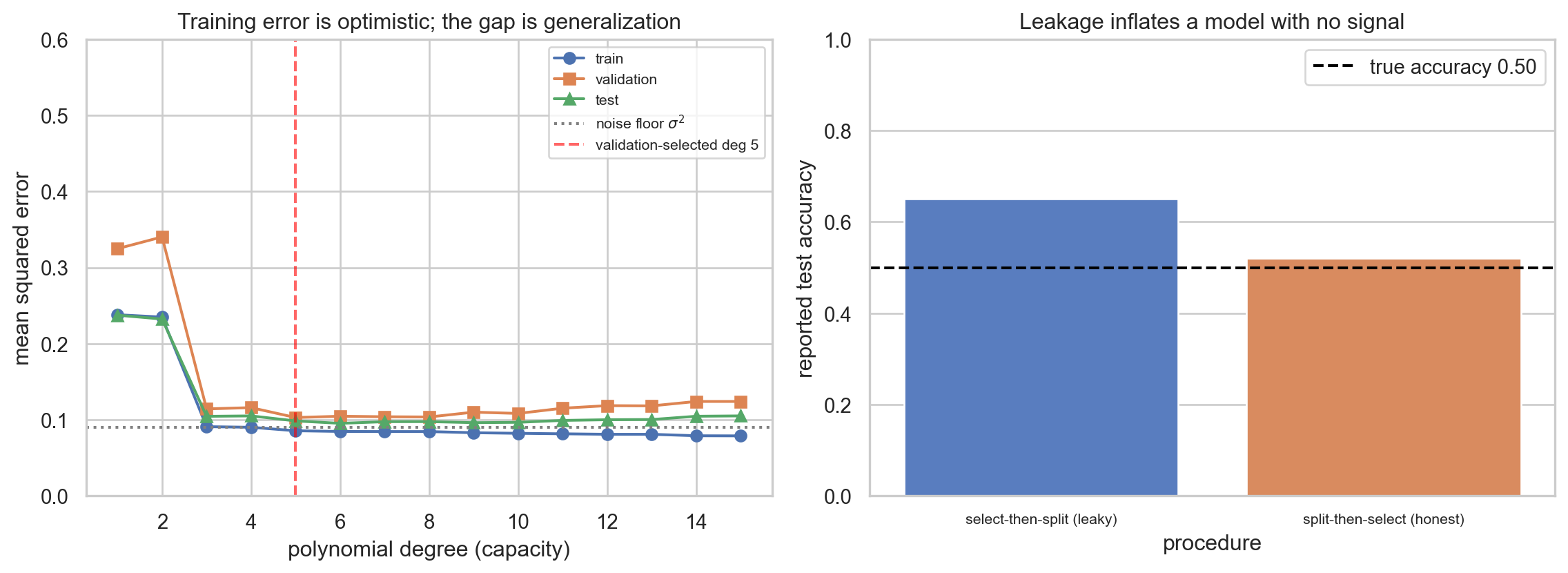
The complexity sweep shows training MSE sliding toward zero as degree rises, while validation and test MSE bottom out near the noise floor \(\sigma^2 = 0.09\) and then climb, the empirical signature of the optimism term \(2\sigma^2 d / n\). The leakage bars show a model built on five noise columns reporting inflated test accuracy when selection precedes the split, and falling back to chance once the split comes first.
using Random, Statistics, Printf

Random.seed!(42)

truef(x) = sin(2pi * x)

n, sigma = 240, 0.30
x = rand(n)
y = truef.(x) .+ sigma .* randn(n)

# Vandermonde design up to a given degree, fit by least squares.
design(xv, d) = reduce(hcat, [xv .^ k for k in 0:d])

idx = shuffle(1:n)
tr, va, te = idx[1:144], idx[145:192], idx[193:240]

@printf("%-7s %-10s %-10s %-10s\n", "degree", "train", "val", "test")
for d in 1:15
    A = design(x[tr], d)
    beta = A \ y[tr]
    mse(s) = mean((design(x[s], d) * beta .- y[s]) .^ 2)
    @printf("%-7d %-10.4f %-10.4f %-10.4f\n", d, mse(tr), mse(va), mse(te))
end
// Illustrative: train/val/test MSE for a polynomial fit via normal equations.
// Uses a tiny Gauss-Jordan solver to keep the example dependency free.
fn solve(mut a: Vec<Vec<f64>>, mut b: Vec<f64>) -> Vec<f64> {
let n = b.len();
for c in 0..n {
let piv = (c..n).max_by(|&i, &j| a[i][c].abs().total_cmp(&a[j][c].abs())).unwrap();
a.swap(c, piv); b.swap(c, piv);
let d = a[c][c];
for j in 0..n { a[c][j] /= d; }
b[c] /= d;
for r in 0..n {
if r != c {
let f = a[r][c];
for j in 0..n { a[r][j] -= f * a[c][j]; }
b[r] -= f * b[c];
}
}
}
b
}
fn design(x: &[f64], d: usize) -> Vec<Vec<f64>> {
x.iter().map(|&xi| (0..=d).map(|k| xi.powi(k as i32)).collect()).collect()
}
fn mse(x: &[f64], y: &[f64], beta: &[f64], d: usize) -> f64 {
design(x, d).iter().zip(y).map(|(row, &yi)| {
let pred: f64 = row.iter().zip(beta).map(|(a, b)| a * b).sum();
(pred - yi).powi(2)
}).sum::<f64>() / y.len() as f64
}
fn main() {
// x, y, and split indices would be filled from data; shown schematically.
let x_tr: Vec<f64> = vec![]; let y_tr: Vec<f64> = vec![];
for d in 1..=15usize {
let a = design(&x_tr, d);
let p = d + 1;
let mut ata = vec![vec![0.0; p]; p];
let mut aty = vec![0.0; p];
for (row, &yi) in a.iter().zip(&y_tr) {
for i in 0..p {
aty[i] += row[i] * yi;
for j in 0..p { ata[i][j] += row[i] * row[j]; }
}
}
if !y_tr.is_empty() {
let beta = solve(ata, aty);
println!("degree {d}: train mse {:.4}", mse(&x_tr, &y_tr, &beta, d));
}
}
}83.9 9. Putting It Together
The three way split is a small idea with large consequences. The training set gives the model its experience, the validation set steers a thousand decisions, and the test set delivers a single honest verdict. Around this skeleton sit the disciplines that keep the verdict honest: split along the true unit of independence to avoid contamination, fit every preprocessing step on training data alone, interrogate features for target leakage, match evaluation distributions to deployment, stratify to tame the variance of small and imbalanced sets, respect the arrow of time when time matters, and guard the test set as a sealed instrument used exactly once. None of these practices improve a model. They ensure that the number you report about a model is true. In a field where it is trivially easy to produce impressive and meaningless metrics, that guarantee is the whole game.
83.10 References
Hastie, T., Tibshirani, R., and Friedman, J. (2009). The Elements of Statistical Learning, 2nd edition. Springer. ISBN 978-0387848570. https://doi.org/10.1007/978-0-387-84858-7
Kaufman, S., Rosset, S., Perlich, C., and Stitelman, O. (2012). Leakage in Data Mining: Formulation, Detection, and Avoidance. ACM Transactions on Knowledge Discovery from Data, 6(4), 1 to 21. https://doi.org/10.1145/2382577.2382579
Kohavi, R. (1995). A Study of Cross Validation and Bootstrap for Accuracy Estimation and Model Selection. Proceedings of the 14th International Joint Conference on Artificial Intelligence (IJCAI), 1137 to 1143. https://dl.acm.org/doi/10.5555/1643031.1643047
Quinonero-Candela, J., Sugiyama, M., Schwaighofer, A., and Lawrence, N. D. (2009). Dataset Shift in Machine Learning. MIT Press. ISBN 978-0262170055. https://doi.org/10.7551/mitpress/9780262170055.001.0001
Sugiyama, M., Krauledat, M., and Muller, K. R. (2007). Covariate Shift Adaptation by Importance Weighted Cross Validation. Journal of Machine Learning Research, 8, 985 to 1005. https://www.jmlr.org/papers/v8/sugiyama07a.html
Dwork, C., Feldman, V., Hardt, M., Pitassi, T., Reingold, O., and Roth, A. (2015). The Reusable Holdout: Preserving Validity in Adaptive Data Analysis. Science, 349(6248), 636 to 638. https://doi.org/10.1126/science.aaa9375
Lopez de Prado, M. (2018). Advances in Financial Machine Learning. Wiley. ISBN 978-1119482086. https://www.wiley.com/en-us/Advances+in+Financial+Machine+Learning-p-9781119482086
Recht, B., Roelofs, R., Schmidt, L., and Shankar, V. (2019). Do ImageNet Classifiers Generalize to ImageNet? Proceedings of the 36th International Conference on Machine Learning (ICML), PMLR 97, 5389 to 5400. https://doi.org/10.48550/arXiv.1902.10811
Pedregosa, F., et al. (2011). Scikit-learn: Machine Learning in Python. Journal of Machine Learning Research, 12, 2825 to 2830. https://www.jmlr.org/papers/v12/pedregosa11a.html
Ng, A. (2018). Machine Learning Yearning. deeplearning.ai. https://info.deeplearning.ai/machine-learning-yearning-book