30  Multivariable Calculus for Machine Learning

Modern machine learning is, at its computational core, an exercise in multivariable calculus. A neural network with billions of parameters defines a scalar loss function over a space of equally many dimensions, and training that network means navigating the geometry of this surface in search of low points. First-order information, the gradient, tells us which direction points downhill, and that single fact powers nearly every optimizer in practice. Yet the gradient alone is silent about the shape of the terrain. To understand why optimization stalls, why some directions are easy and others treacherous, and why the high-dimensional loss landscapes of deep networks behave so differently from the low-dimensional intuition we carry from calculus class, we need second-order information. This chapter develops the Hessian matrix, the multivariable Taylor expansion, the classification of critical points, and the curvature of loss landscapes, and it connects each idea back to the practical business of training models.

30.1 1. From Gradients to the Hessian

30.1.1 1.1 The Gradient as a Linear Approximation

Consider a scalar function \(f : \mathbb{R}^n \to \mathbb{R}\), which we treat as a loss \(L(\theta)\) over a parameter vector \(\theta\). The gradient is the vector of first partial derivatives,

\[ \nabla f(\mathbf{x}) = \left( \frac{\partial f}{\partial x_1}, \frac{\partial f}{\partial x_2}, \ldots, \frac{\partial f}{\partial x_n} \right)^\top. \]

The gradient is the best linear model of \(f\) near a point. For a small displacement \(\mathbf{v}\), the directional derivative \(\nabla f(\mathbf{x})^\top \mathbf{v}\) gives the instantaneous rate of change of \(f\) along \(\mathbf{v}\). Because this is an inner product, it is maximized when \(\mathbf{v}\) aligns with \(\nabla f\), which is exactly why steepest ascent moves along the gradient and gradient descent moves against it. The gradient is geometrically a vector that is orthogonal to the level sets of \(f\), pointing toward steeper values.

The trouble is that a linear model captures only slope, not bending. Two loss surfaces can share an identical gradient at a point while curving in completely different ways, and that curvature governs how a step of a given size will actually behave. To see it we differentiate once more.

30.1.2 1.2 Definition of the Hessian Matrix

The Hessian is the matrix of all second-order partial derivatives. For \(f : \mathbb{R}^n \to \mathbb{R}\) it is the \(n \times n\) matrix

\[ H(\mathbf{x}) = \nabla^2 f(\mathbf{x}), \qquad H_{ij} = \frac{\partial^2 f}{\partial x_i \, \partial x_j}. \]

Each diagonal entry \(H_{ii}\) measures how the slope in coordinate \(i\) changes as we move along coordinate \(i\), that is, the pure curvature in that axis. Each off-diagonal entry \(H_{ij}\) measures how the slope in coordinate \(i\) changes as we move along coordinate \(j\), capturing the way the parameters interact.

A central structural fact is symmetry. When the second partial derivatives are continuous, Clairaut’s theorem (also called Schwarz’s theorem) guarantees that the order of differentiation does not matter,

\[ \frac{\partial^2 f}{\partial x_i \, \partial x_j} = \frac{\partial^2 f}{\partial x_j \, \partial x_i}, \]

so \(H = H^\top\). Symmetry is not a cosmetic convenience. It guarantees that the Hessian has a full set of real eigenvalues and an orthonormal basis of eigenvectors, by the spectral theorem. Those eigenvalues and eigenvectors are the language in which we will describe the entire local geometry of a loss landscape.

30.1.3 1.3 The Hessian as Curvature

The eigendecomposition \(H = Q \Lambda Q^\top\) resolves the curvature into principal axes. Each eigenvector \(\mathbf{q}_k\) is a direction in parameter space, and its eigenvalue \(\lambda_k\) is the curvature of the loss along that direction. A large positive \(\lambda_k\) means the loss rises sharply as you move along \(\mathbf{q}_k\), like the steep wall of a narrow valley. A small or zero eigenvalue means the loss is nearly flat in that direction. A negative eigenvalue means the loss curves downward, so that direction leads to lower values. This spectral picture is the workhorse of everything that follows.

30.2 2. The Multivariable Taylor Expansion

30.2.1 2.1 The Second-Order Expansion

The Taylor expansion is the bridge between the gradient, the Hessian, and the local shape of the function. Around a point \(\mathbf{x}_0\), for a displacement \(\mathbf{v}\),

\[ f(\mathbf{x}_0 + \mathbf{v}) = f(\mathbf{x}_0) + \nabla f(\mathbf{x}_0)^\top \mathbf{v} + \tfrac{1}{2} \mathbf{v}^\top H(\mathbf{x}_0) \, \mathbf{v} + O(\|\mathbf{v}\|^3). \]

Read this term by term. The constant \(f(\mathbf{x}_0)\) is the current loss. The linear term \(\nabla f(\mathbf{x}_0)^\top \mathbf{v}\) is the first-order change, the part that gradient descent reasons about. The quadratic term \(\tfrac{1}{2}\mathbf{v}^\top H \mathbf{v}\) is the curvature correction, the leading contribution that the gradient ignores. Truncating after the quadratic term approximates the loss surface by a paraboloid, and that paraboloid is the model that second-order optimization methods optimize exactly at each step.

30.2.2 2.2 Deriving the Expansion

The multivariable expansion follows from the single-variable Taylor theorem applied along a line. Fix \(\mathbf{x}_0\) and a direction \(\mathbf{v}\), and define the scalar function \(g(t) = f(\mathbf{x}_0 + t\mathbf{v})\) for \(t \in [0,1]\). This restricts \(f\) to the segment joining \(\mathbf{x}_0\) to \(\mathbf{x}_0 + \mathbf{v}\). By the chain rule, the first derivative is the directional derivative,

\[ g'(t) = \nabla f(\mathbf{x}_0 + t\mathbf{v})^\top \mathbf{v} = \sum_{i=1}^{n} \frac{\partial f}{\partial x_i} \, v_i, \]

and differentiating once more, again by the chain rule applied to each partial derivative,

\[ g''(t) = \sum_{i=1}^{n} \sum_{j=1}^{n} \frac{\partial^2 f}{\partial x_i \, \partial x_j} \, v_i v_j = \mathbf{v}^\top H(\mathbf{x}_0 + t\mathbf{v}) \, \mathbf{v}. \]

The scalar Taylor theorem with the Lagrange remainder gives \(g(1) = g(0) + g'(0) + \tfrac{1}{2} g''(\xi)\) for some \(\xi \in (0,1)\). Substituting the expressions above and noting that \(g(1) = f(\mathbf{x}_0 + \mathbf{v})\) and \(g(0) = f(\mathbf{x}_0)\) yields the exact second-order form,

\[ f(\mathbf{x}_0 + \mathbf{v}) = f(\mathbf{x}_0) + \nabla f(\mathbf{x}_0)^\top \mathbf{v} + \tfrac{1}{2}\, \mathbf{v}^\top H(\mathbf{x}_0 + \xi \mathbf{v}) \, \mathbf{v}. \]

When \(H\) is continuous, replacing \(H(\mathbf{x}_0 + \xi \mathbf{v})\) by \(H(\mathbf{x}_0)\) introduces an error of order \(\|\mathbf{v}\|^3\), which recovers the truncated expansion. The derivation shows precisely where the Hessian enters: it is the second derivative of \(f\) along every line through the point, assembled into a single matrix by the bilinear form \(\mathbf{v}^\top H \mathbf{v}\).

30.2.3 2.3 The Quadratic Form and Its Meaning

The expression \(\mathbf{v}^\top H \mathbf{v}\) is a quadratic form, and using the eigendecomposition we can rewrite it in the eigenbasis. Writing \(\mathbf{v} = \sum_k c_k \mathbf{q}_k\) with coefficients \(c_k = \mathbf{q}_k^\top \mathbf{v}\), we get

\[ \mathbf{v}^\top H \mathbf{v} = \sum_{k=1}^{n} \lambda_k \, c_k^2. \]

The curvature experienced along a direction is a weighted sum of the eigenvalues, weighted by how much that direction projects onto each eigenvector. Along a pure eigenvector \(\mathbf{q}_k\) the curvature is exactly \(\lambda_k\). This decomposition makes the geometry concrete. If all \(\lambda_k > 0\) the paraboloid is a bowl that opens upward in every direction. If all \(\lambda_k < 0\) it is a dome. If the eigenvalues have mixed signs, the surface bends up in some directions and down in others, which is the defining feature of a saddle.

30.2.4 2.4 Why the Quadratic Model Matters for Steps

Suppose we take a gradient step \(\mathbf{v} = -\eta \nabla f\) with learning rate \(\eta\). Substituting into the quadratic model and minimizing over \(\eta\) shows that the safe step size is controlled by the largest eigenvalue of the Hessian. If \(\eta\) exceeds roughly \(2 / \lambda_{\max}\), the step overshoots in the sharpest direction and the loss diverges. Meanwhile progress in the flattest direction proceeds at a rate governed by \(\lambda_{\min}\). The ratio \(\kappa = \lambda_{\max} / \lambda_{\min}\), the condition number, therefore measures how badly the two requirements conflict. A large condition number forces a small learning rate to stay stable in steep directions, which leaves the flat directions crawling. This single quantity explains much of the pain of training poorly conditioned models.

30.3 3. Critical Points and the Second-Derivative Test

30.3.1 3.1 Critical Points

A critical point (or stationary point) is a location where the gradient vanishes,

\[ \nabla f(\mathbf{x}^*) = \mathbf{0}. \]

At such a point the linear term of the Taylor expansion disappears, and the local behavior is governed entirely by the quadratic term \(\tfrac{1}{2}\mathbf{v}^\top H \mathbf{v}\). Every minimum, maximum, and saddle of the loss is a critical point, and optimizers that follow the gradient come to rest exactly at these points. Classifying them is therefore the key to understanding where training converges and whether that destination is good.

30.3.2 3.2 The Second-Derivative Test

The sign structure of the Hessian’s eigenvalues classifies a critical point. We say \(H\) is positive definite if \(\mathbf{v}^\top H \mathbf{v} > 0\) for all nonzero \(\mathbf{v}\), which holds exactly when every eigenvalue is positive. The test reads as follows.

• If \(H(\mathbf{x}^*)\) is positive definite, all \(\lambda_k > 0\), and \(\mathbf{x}^*\) is a local minimum. The surface curves upward in every direction.
• If \(H(\mathbf{x}^*)\) is negative definite, all \(\lambda_k < 0\), and \(\mathbf{x}^*\) is a local maximum.
• If \(H(\mathbf{x}^*)\) has both positive and negative eigenvalues, it is indefinite, and \(\mathbf{x}^*\) is a saddle point.
• If \(H(\mathbf{x}^*)\) is positive or negative semidefinite with at least one zero eigenvalue, the test is inconclusive, and the third-order terms must be examined to decide the behavior in the flat direction.

In two dimensions this reduces to the familiar discriminant rule, where the sign of \(\det H = \lambda_1 \lambda_2\) and the sign of the trace decide the case. In high dimensions the eigenvalue picture is the only practical way to think.

Why definiteness decides the case (proof sketch). At a critical point the gradient vanishes, so the Taylor expansion collapses to

\[ f(\mathbf{x}^* + \mathbf{v}) - f(\mathbf{x}^*) = \tfrac{1}{2}\, \mathbf{v}^\top H \, \mathbf{v} + O(\|\mathbf{v}\|^3). \]

The sign of the loss change for small \(\mathbf{v}\) is therefore the sign of the quadratic form \(\mathbf{v}^\top H \mathbf{v}\), provided that form is not zero. Diagonalize in the eigenbasis, \(\mathbf{v}^\top H \mathbf{v} = \sum_k \lambda_k c_k^2\) with \(c_k = \mathbf{q}_k^\top \mathbf{v}\). If every \(\lambda_k > 0\), then \(\sum_k \lambda_k c_k^2 \geq \lambda_{\min}\|\mathbf{v}\|^2 > 0\) for all nonzero \(\mathbf{v}\), so the loss strictly increases in every direction and \(\mathbf{x}^*\) is a strict local minimum; the cubic remainder cannot overturn a strictly positive quadratic term once \(\|\mathbf{v}\|\) is small enough, since it shrinks faster. The negative definite case is identical with the sign flipped, giving a maximum. If \(H\) is indefinite, pick an eigenvector \(\mathbf{q}_+\) with \(\lambda_+ > 0\) and another \(\mathbf{q}_-\) with \(\lambda_- < 0\): moving along \(\mathbf{q}_+\) raises the loss while moving along \(\mathbf{q}_-\) lowers it, so the point is neither a minimum nor a maximum but a saddle. When some \(\lambda_k = 0\), the quadratic term vanishes along that eigenvector and the leading nonzero behavior is set by third- or higher-order terms, which is why the test is inconclusive there.

30.3.3 3.3 An Illustrative Example

Take \(f(x, y) = x^2 - y^2\). Its gradient is \((2x, -2y)\), which vanishes only at the origin. The Hessian is constant,

\[ H = \begin{pmatrix} 2 & 0 \\ 0 & -2 \end{pmatrix}, \]

with eigenvalues \(+2\) and \(-2\). The mixed signs flag the origin as a saddle. Moving along the \(x\) axis the function increases, moving along the \(y\) axis it decreases, and the origin is a minimum in one slice and a maximum in another. This is the prototype of the structure that dominates high-dimensional loss surfaces.

30.4 4. Curvature of Loss Landscapes

30.4.1 4.1 What the Hessian Tells Us About Training

For a loss \(L(\theta)\), the Hessian at the current parameters describes the local terrain that the optimizer must traverse. The eigenvalue spectrum of \(H\) has a characteristic shape in trained neural networks. Empirically the spectrum is dominated by a bulk of eigenvalues clustered near zero, indicating many nearly flat directions, together with a small number of large outlier eigenvalues that capture the few sharply curved directions. This means the loss surface near a solution looks like a long thin valley, gently sloped along most axes and steeply walled along a few.

The flat directions are not a nuisance to be eliminated. They form connected regions of near-constant loss and are closely tied to why overparameterized networks generalize and why many distinct parameter settings achieve similar performance. The sharp directions, by contrast, dictate stability and the maximum usable learning rate.

30.4.2 4.2 Sharpness, Flatness, and Generalization

The curvature around a minimum has been linked to how well a model generalizes. A flat minimum, one where the eigenvalues of the Hessian are small, sits in a wide basin where small perturbations of the parameters barely change the loss. A sharp minimum sits in a narrow basin where the same perturbation causes a large loss increase. A long line of work argues, with both intuition and evidence, that flatter minima tend to generalize better, because a wide basin is more robust to the mismatch between the training loss and the test loss. This insight has been operationalized directly. Sharpness Aware Minimization (SAM) modifies the training objective to seek parameters whose entire neighborhood has low loss, explicitly preferring flat regions, and it improves generalization across many benchmarks. Curvature, an object defined purely by multivariable calculus, becomes a lever on model quality.

30.4.3 4.3 Conditioning and the Geometry of Descent

Recall the condition number \(\kappa = \lambda_{\max}/\lambda_{\min}\) over the nonzero spectrum. To see why it controls convergence, consider gradient descent with step size \(\eta\) on the quadratic model \(f(\mathbf{x}) = \tfrac{1}{2}\mathbf{x}^\top H \mathbf{x}\). In the eigenbasis the iteration decouples coordinate by coordinate, and the component along \(\mathbf{q}_k\) obeys

\[ c_k^{(t+1)} = (1 - \eta \lambda_k)\, c_k^{(t)}, \]

so each coordinate contracts by the factor \(|1 - \eta \lambda_k|\) per step. Stability in the sharpest direction requires \(\eta < 2/\lambda_{\max}\), while the slowest contraction occurs along \(\lambda_{\min}\). Choosing the optimal \(\eta\) that balances the two extremes gives a worst-case contraction factor of \((\kappa - 1)/(\kappa + 1)\) per step, so the number of iterations to reach a fixed accuracy scales linearly with \(\kappa\). Gradient descent on an ill-conditioned quadratic zigzags, bouncing across the steep walls of the valley while creeping along its floor. This geometric fact motivates a great deal of practical machinery. Momentum dampens the oscillations across steep directions and accelerates the slow drift along flat ones. Adaptive methods such as Adam rescale each coordinate by an estimate of its own curvature or gradient magnitude, which is an attempt to reduce the effective condition number without ever forming the full Hessian. Normalization layers reshape the loss surface so that its curvature is more uniform. Each of these is a response to the spectrum of \(H\).

30.5 5. Saddle Points in High Dimensions

30.5.1 5.1 Why Saddles Dominate

In low dimensions our intuition says that a critical point is usually a minimum or a maximum, and saddles feel like rare curiosities. High dimensions overturn this intuition. For a critical point to be a local minimum, every one of the \(n\) eigenvalues of the Hessian must be positive. If we picture the signs of the eigenvalues as roughly independent coin flips, the probability that all \(n\) land positive shrinks exponentially as \(n\) grows. Critical points with a mix of positive and negative eigenvalues, which are saddles, become overwhelmingly the most common type. Results from the statistical physics of random Gaussian fields make this precise and show that low critical points are increasingly likely to be minima while high critical points are saddles, with an index that grows smoothly with the loss value.

The consequence for deep learning is that the obstacles to optimization are mostly saddle points rather than poor local minima. The historically feared scenario of getting stuck in a bad local minimum is, in very high dimensions, far less common than getting slowed near a saddle.

30.5.2 5.2 How Saddles Slow Optimization

Near a saddle the gradient is small because we are close to a critical point, yet the point is not a solution. Gradient descent slows to a crawl precisely where it should be escaping, because the descending directions, the eigenvectors with negative eigenvalues, contribute only weakly to the gradient when the iterate sits near the saddle. The optimizer can spend many iterations on the plateau surrounding the saddle before it finds and follows a downhill eigenvector. Plateaus in the training loss curve often correspond to exactly this phenomenon.

30.5.3 5.3 Escaping Saddles

Understanding saddles points to ways past them. Second-order methods can detect a negative eigenvalue of the Hessian and move along the corresponding eigenvector to descend, which is the strategy behind saddle-free Newton methods that use the absolute value of the Hessian eigenvalues to take well-scaled steps in every direction. More simply, the stochastic noise inherent in minibatch gradient estimates perturbs the iterate off the plateau and tends to push it toward a descending direction, so plain stochastic gradient descent escapes most saddles given enough time. Theoretical work shows that gradient methods with a little injected noise escape strict saddle points efficiently, which helps explain why the saddle-rich landscapes of deep networks are nonetheless trainable in practice.

30.6 6. Classifying a Critical Point in Code

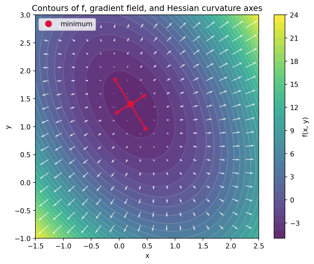
The ideas of this chapter are concrete enough to compute directly. The example below defines a scalar function \(f(x, y)\), finds its critical point by solving \(\nabla f = \mathbf{0}\), classifies that point through the eigenvalues of the Hessian, reports the condition number, and checks that the second-order Taylor model is exact for a quadratic. The same recipe scales to any twice-differentiable loss: form the Hessian, read its spectrum, and the local geometry follows.

30.6.1 Python (executable)

import numpy as np

np.random.seed(0)

# Define a scalar function f(x, y) and its analytic gradient and Hessian.
def f(p):
    x, y = p
    return 3.0 * x**2 + 2.0 * x * y + 2.0 * y**2 - 4.0 * x - 6.0 * y

def grad(p):
    x, y = p
    return np.array([6.0 * x + 2.0 * y - 4.0,
                     2.0 * x + 4.0 * y - 6.0])

# The Hessian is constant for this quadratic.
H = np.array([[6.0, 2.0],
              [2.0, 4.0]])

# Critical point: solve grad = 0  ->  H @ p = b
b = np.array([4.0, 6.0])
p_star = np.linalg.solve(H, b)
print("Critical point (grad = 0):", np.round(p_star, 6))
print("Gradient at critical point:", np.round(grad(p_star), 10))

# Classify via Hessian eigenvalues.
eigvals, eigvecs = np.linalg.eigh(H)
print("Hessian eigenvalues:", np.round(eigvals, 6))
kappa = eigvals.max() / eigvals.min()
print("Condition number kappa:", round(kappa, 6))

if np.all(eigvals > 0):
    kind = "local minimum (positive definite)"
elif np.all(eigvals < 0):
    kind = "local maximum (negative definite)"
else:
    kind = "saddle point (indefinite)"
print("Classification:", kind)

# Verify the second-order Taylor model is exact for a quadratic.
x0 = np.array([0.5, -0.5])
v = np.array([0.3, 0.4])
exact = f(x0 + v)
model = f(x0) + grad(x0) @ v + 0.5 * v @ H @ v
print("Exact f(x0+v):", round(float(exact), 6))
print("Taylor model:", round(float(model), 6))
print("Match:", np.isclose(exact, model))

# Figure: contour plot of f with its gradient field, plus the eigenvectors
# of the Hessian at the minimum showing the steep and flat curvature axes.
import matplotlib.pyplot as plt

xs = np.linspace(-1.5, 2.5, 400)
ys = np.linspace(-1.0, 3.0, 400)
X, Y = np.meshgrid(xs, ys)
Z = 3.0 * X**2 + 2.0 * X * Y + 2.0 * Y**2 - 4.0 * X - 6.0 * Y

# Coarser grid for the gradient (quiver) field.
gx = np.linspace(-1.5, 2.5, 18)
gy = np.linspace(-1.0, 3.0, 18)
GX, GY = np.meshgrid(gx, gy)
U = 6.0 * GX + 2.0 * GY - 4.0
V = 2.0 * GX + 4.0 * GY - 6.0

fig, ax = plt.subplots(figsize=(7.0, 5.5))
cs = ax.contourf(X, Y, Z, levels=30, cmap="viridis", alpha=0.85)
ax.contour(X, Y, Z, levels=30, colors="white", linewidths=0.4, alpha=0.5)
fig.colorbar(cs, ax=ax, label="f(x, y)")

# Gradient field (points uphill, perpendicular to the level curves).
ax.quiver(GX, GY, U, V, color="white", alpha=0.8, width=0.003)

# Mark the minimum and draw the Hessian eigenvectors, scaled so the steep
# direction (large eigenvalue) appears shorter for the same energy step.
ax.plot(p_star[0], p_star[1], "o", color="crimson", markersize=9,
        label="minimum")
for val, vec in zip(eigvals, eigvecs.T):
    step = vec / np.sqrt(val)
    ax.annotate("", xy=p_star + step, xytext=p_star - step,
                arrowprops=dict(arrowstyle="<->", color="crimson", lw=2.0))

ax.set_xlabel("x")
ax.set_ylabel("y")
ax.set_title("Contours of f, gradient field, and Hessian curvature axes")
ax.legend(loc="upper left")
ax.set_aspect("equal")
fig.tight_layout()
plt.show()

Critical point (grad = 0): [0.2 1.4]
Gradient at critical point: [0. 0.]
Hessian eigenvalues: [2.763932 7.236068]
Condition number kappa: 2.618034
Classification: local minimum (positive definite)
Exact f(x0+v): -0.82
Taylor model: -0.82
Match: True

The eigenvalues come out both positive, so the critical point is a local minimum, and the condition number near \(2.6\) quantifies how much steeper the sharp direction is than the flat one. Because \(f\) is exactly quadratic, the truncated Taylor model reproduces the function value with no error, which is the limiting case the second-order expansion describes.

30.6.2 Julia

using LinearAlgebra

# Hessian (constant for this quadratic) and the right-hand side of grad = 0.
H = [6.0 2.0; 2.0 4.0]
b = [4.0, 6.0]

p_star = H \ b
println("Critical point: ", round.(p_star, digits=6))

vals = eigvals(H)
println("Hessian eigenvalues: ", round.(vals, digits=6))
println("Condition number: ", round(maximum(vals) / minimum(vals), digits=6))

kind = all(vals .> 0) ? "local minimum" :
       all(vals .< 0) ? "local maximum" : "saddle point"
println("Classification: ", kind)

30.6.3 Rust (illustrative)

// Classify a 2x2 symmetric Hessian by its eigenvalues.
// Illustrative: eigenvalues of [[a, b], [b, d]] in closed form.
fn eigenvalues(a: f64, b: f64, d: f64) -> (f64, f64) {
    let tr = a + d;
    let disc = ((a - d).powi(2) + 4.0 * b * b).sqrt();
    ((tr - disc) / 2.0, (tr + disc) / 2.0)
}

fn main() {
    let (a, b, d) = (6.0, 2.0, 4.0);
    let (lo, hi) = eigenvalues(a, b, d);
    println!("Eigenvalues: {:.6}, {:.6}", lo, hi);
    println!("Condition number: {:.6}", hi / lo);

    let kind = if lo > 0.0 && hi > 0.0 {
        "local minimum"
    } else if lo < 0.0 && hi < 0.0 {
        "local maximum"
    } else {
        "saddle point"
    };
    println!("Classification: {}", kind);
}

30.7 7. How This Informs Optimization

30.7.1 7.1 Newton’s Method and Its Approximations

The cleanest use of second-order information is Newton’s method. Minimizing the second-order Taylor model exactly gives the step

\[ \mathbf{v} = -H^{-1} \nabla f, \]

which rescales the gradient by the inverse curvature. In the eigenbasis this divides the gradient component along each direction by that direction’s eigenvalue, so steep directions take small steps and flat directions take large ones, neutralizing the condition number entirely. The catch is that forming and inverting an \(n \times n\) Hessian is impossible when \(n\) runs into the billions, and near saddles the raw Newton step can move toward the saddle rather than away. Practical second-order optimization therefore relies on approximations. Quasi-Newton methods such as L-BFGS build a low-memory estimate of the inverse Hessian from gradient history. Gauss-Newton and natural gradient methods replace the true Hessian with a positive semidefinite surrogate that is cheaper and avoids the negative-curvature pathology. Kronecker-factored approximations such as K-FAC exploit network structure to approximate the curvature block by block.

30.7.2 7.2 Curvature Without the Full Matrix

A recurring theme is that we rarely need the full Hessian, only its action. The Hessian-vector product \(H \mathbf{v}\) can be computed at roughly the cost of a single gradient evaluation, without ever materializing \(H\), by differentiating the gradient in the direction \(\mathbf{v}\). This trick underlies efficient estimation of the top eigenvalues, the trace, and conjugate-gradient solves of the Newton system. It is the reason curvature can be studied and partly exploited at the scale of modern models. Diagnostic tools that estimate \(\lambda_{\max}\) of the Hessian during training, for instance, let practitioners reason directly about stability and learning-rate limits.

30.7.3 7.3 The Practical Takeaway

The progression from gradient to Hessian to spectrum is the throughline of this chapter, and it pays off as a way of reasoning about training. When loss diverges, suspect a learning rate above the stability limit set by \(\lambda_{\max}\). When training stalls on a plateau, suspect a saddle and lean on stochastic noise or curvature-aware steps to escape. When a model trains but fails to generalize, consider the sharpness of the minimum it found. When progress is steady but slow, suspect poor conditioning and reach for momentum, adaptive scaling, or normalization. Each diagnosis is a statement about the eigenvalues of the Hessian, and each remedy is a way of acting on the second-order geometry that the multivariable Taylor expansion makes visible. First-order methods will continue to do the heavy lifting of large-scale training, but it is second-order information that explains why they succeed, why they fail, and how to make them better.

30.8 References

1. Goodfellow, I., Bengio, Y., and Courville, A. (2016). Deep Learning. MIT Press. https://www.deeplearningbook.org/

2. Boyd, S. and Vandenberghe, L. (2004). Convex Optimization. Cambridge University Press. https://doi.org/10.1017/CBO9780511804441

3. Nocedal, J. and Wright, S. J. (2006). Numerical Optimization, 2nd edition. Springer. https://doi.org/10.1007/978-0-387-40065-5

4. Dauphin, Y. N., Pascanu, R., Gulcehre, C., Cho, K., Ganguli, S., and Bengio, Y. (2014). Identifying and attacking the saddle point problem in high-dimensional non-convex optimization. Advances in Neural Information Processing Systems (NeurIPS) 27. https://doi.org/10.48550/arXiv.1406.2572

5. Choromanska, A., Henaff, M., Mathieu, M., Ben Arous, G., and LeCun, Y. (2015). The loss surfaces of multilayer networks. Proceedings of the 18th International Conference on Artificial Intelligence and Statistics (AISTATS), PMLR 38, 192-204. https://proceedings.mlr.press/v38/choromanska15.html

6. Ge, R., Huang, F., Jin, C., and Yuan, Y. (2015). Escaping from saddle points: online stochastic gradient for tensor decomposition. Proceedings of the 28th Conference on Learning Theory (COLT), PMLR 40, 797-842. https://proceedings.mlr.press/v40/Ge15.html

7. Jin, C., Ge, R., Netrapalli, P., Kakade, S. M., and Jordan, M. I. (2017). How to escape saddle points efficiently. Proceedings of the 34th International Conference on Machine Learning (ICML), PMLR 70, 1724-1732. https://proceedings.mlr.press/v70/jin17a.html

8. Keskar, N. S., Mudigere, D., Nocedal, J., Smelyanskiy, M., and Tang, P. T. P. (2017). On large-batch training for deep learning: generalization gap and sharp minima. International Conference on Learning Representations (ICLR). https://doi.org/10.48550/arXiv.1609.04836

9. Foret, P., Kleiner, A., Mobahi, H., and Neyshabur, B. (2021). Sharpness-Aware Minimization for efficiently improving generalization. International Conference on Learning Representations (ICLR). https://doi.org/10.48550/arXiv.2010.01412

10. Martens, J. and Grosse, R. (2015). Optimizing neural networks with Kronecker-factored approximate curvature. Proceedings of the 32nd International Conference on Machine Learning (ICML), PMLR 37, 2408-2417. https://proceedings.mlr.press/v37/martens15.html

11. Pearlmutter, B. A. (1994). Fast exact multiplication by the Hessian. Neural Computation, 6(1), 147-160. https://doi.org/10.1162/neco.1994.6.1.147

12. Ghorbani, B., Krishnan, S., and Xiao, Y. (2019). An investigation into neural net optimization via Hessian eigenvalue density. Proceedings of the 36th International Conference on Machine Learning (ICML), PMLR 97, 2232-2241. https://proceedings.mlr.press/v97/ghorbani19b.html