K-means is the most widely used clustering algorithm in practice, and for good reason: it is simple to state, fast to run, and yields a partition that is easy to interpret. Beneath that simplicity lies a rich optimization problem with subtle geometry. This chapter develops the objective that k-means minimizes, the iterative procedure (Lloyd’s algorithm) that descends on it, the seeding scheme (k-means++) that makes the procedure reliable, and the theory around convergence, model selection, and the assumptions the method silently encodes. The goal is to leave you able to apply k-means with judgment rather than as a black box.
128.1 1. The Clustering Objective
128.1.1 1.1 Problem statement
We are given \(n\) data points \(x_1, \dots, x_n \in \mathbb{R}^d\) and a target number of clusters \(k\). We seek a partition of the points into \(k\) disjoint sets \(C_1, \dots, C_k\) together with a set of representatives, called centroids, \(\mu_1, \dots, \mu_k \in \mathbb{R}^d\). K-means defines the quality of such an assignment through the within-cluster sum of squares, also called inertia or distortion:
The objective rewards partitions in which every point sits close, in squared Euclidean distance, to the centroid of its assigned cluster. Minimizing \(J\) over both the assignment \(C\) and the centroids \(\mu\) is the k-means problem.
128.1.2 1.2 Why squared Euclidean distance
The choice of squared \(\ell_2\) distance is not cosmetic; it is what makes the centroid the optimal representative. Fix a cluster \(C_j\) and ask which point \(\mu_j\) minimizes \(\sum_{x_i \in C_j} \lVert x_i - \mu_j \rVert_2^2\). Setting the gradient to zero gives
The minimizer is exactly the arithmetic mean, which is where the name k-means comes from. If we instead used the \(\ell_1\) distance, the optimal representative would be the coordinatewise median, giving the k-medians algorithm; if we restricted representatives to be actual data points, we would get k-medoids. The squared norm also yields a useful identity: the total inertia equals the sum over clusters of \(|C_j|\) times the variance within \(C_j\), so k-means can be read as variance minimization.
128.1.3 1.3 Computational hardness
Despite its simple form, exactly minimizing \(J\) is NP-hard. The difficulty holds even for \(k = 2\) clusters in general dimension, and separately for fixed dimension \(d = 2\) with general \(k\). There are roughly \(k^n / k!\) ways to partition \(n\) points into \(k\) nonempty groups, an astronomical search space. We therefore do not solve k-means exactly. We rely on local-search heuristics that find good partitions quickly, accepting that they may not reach the global optimum. Lloyd’s algorithm is the canonical such heuristic.
128.2 2. Lloyd’s Algorithm
128.2.1 2.1 Coordinate descent on two variables
The objective \(J(C, \mu)\) depends on two groups of variables: the discrete assignments \(C\) and the continuous centroids \(\mu\). Lloyd’s algorithm performs alternating minimization, optimizing one group while holding the other fixed.
Assignment step. With centroids fixed, the objective decomposes across points: each \(x_i\) contributes \(\min_j \lVert x_i - \mu_j \rVert^2\) to the total if assigned optimally. The best move is to assign every point to its nearest centroid:
We iterate these two steps until the assignments stop changing.
initialize centroids mu_1 ... mu_k
repeat:
    # assignment step
    for each point x_i:
        c_i = index of nearest centroid
    # update step
    for each cluster j:
        mu_j = mean of points assigned to j
until assignments unchanged
We can run this on synthetic data. We generate four well-separated blobs and let scikit-learn’s k-means (which implements Lloyd’s algorithm) partition them, then report the recovered cluster sizes, the final inertia, and how many iterations convergence took.
Cluster sizes: [75 75 75 75]
Final inertia: 362.47
Iterations to converge: 3
The four true clusters are each recovered with their full membership, and the algorithm settles in only a few iterations.
128.2.2 2.2 Monotone descent and finite termination
Each step weakly decreases \(J\). The assignment step lowers (or holds) every point’s contribution because reassigning to the nearest centroid can only shrink its squared distance. The update step lowers (or holds) each cluster’s contribution because the mean is the unique minimizer of within-cluster squared distance. Therefore the sequence of objective values is nonincreasing.
Because there are only finitely many distinct assignments (at most \(k^n\)), and the objective strictly decreases whenever an assignment changes, the algorithm cannot cycle and must terminate after a finite number of iterations. In practice it usually converges in a few dozen iterations or fewer, though contrived inputs can force a number of iterations exponential in \(n\). The smoothed complexity is polynomial, which explains why the worst case almost never appears on real data.
128.2.3 2.3 Cost per iteration
A single iteration computes the distance from each of \(n\) points to each of \(k\) centroids in \(d\) dimensions, costing \(O(nkd)\) time. The update step is also \(O(nd)\) since it is one pass to accumulate sums. With \(T\) iterations the total is \(O(nkdT)\), linear in the number of points. This scalability is the practical reason k-means dominates: it handles large \(n\) where most clustering methods, which need pairwise distances at \(O(n^2)\) cost, cannot.
128.2.4 2.4 Empty clusters
A subtlety: the update step assumes every cluster is nonempty. If a centroid ends up with no assigned points, its mean is undefined. Standard implementations handle this by reseeding the empty centroid, for instance to the point that is currently farthest from its assigned centroid, which both repairs the partition and tends to reduce the objective.
128.3 3. The k-means++ Initialization
128.3.1 3.1 Why initialization matters
Lloyd’s algorithm converges only to a local minimum, and which local minimum it reaches depends entirely on the starting centroids. Naive initialization, sampling \(k\) points uniformly at random, frequently places two seeds in the same dense region and none in another, producing a poor partition that no amount of iterating can escape. The standard remedy is to run Lloyd from many random starts and keep the best, but that wastes computation and still offers no guarantee.
128.3.2 3.2 The seeding procedure
K-means++ replaces uniform seeding with a careful, adaptive sampling scheme that spreads the initial centroids out. It chooses the first center uniformly at random, then chooses each subsequent center with probability proportional to its squared distance from the nearest already-chosen center.
choose c_1 uniformly at random from the data
for j = 2 ... k:
    for each point x_i:
        D(x_i) = distance to nearest already-chosen center
    choose c_j = x_i with probability proportional to D(x_i)^2
run Lloyd's algorithm from these k centers
The intuition is that a point far from all current centers is precisely a point that the current seeding represents poorly, so it is a strong candidate to anchor a new cluster. The squared weighting biases selection toward such points while retaining randomness, which prevents the procedure from always grabbing outliers.
128.3.3 3.3 The approximation guarantee
The reason k-means++ is more than a heuristic is its provable guarantee. Let \(J^\star\) be the optimal value of the k-means objective. The expected cost of the partition obtained right after k-means++ seeding, before any Lloyd iterations, satisfies
The seeding alone is \(O(\log k)\)-competitive with the global optimum in expectation. Running Lloyd’s algorithm afterward only improves on this. The practical effect is dramatic: k-means++ typically reaches a lower final objective, converges in fewer iterations, and exhibits far less variance across random seeds than uniform initialization. It is the default initializer in essentially every mature k-means library, and it is what you should use unless you have a specific reason not to.
128.3.4 3.4 Scalable variants
The sequential nature of k-means++ requires \(k\) passes over the data, which becomes a bottleneck at very large scale. The variant k-means|| (k-means parallel) oversamples several candidate centers per round across a constant number of rounds, then reclusters the candidate set down to \(k\) centers. It retains a similar approximation quality while parallelizing cleanly across a distributed dataset.
128.4 4. Convergence and Local Minima
128.4.1 4.1 What convergence does and does not promise
Lloyd’s algorithm converges in the sense that the objective stops decreasing and the assignments stabilize. It does not promise that the resulting partition is globally optimal, or even close. The fixed points of the iteration are the partitions where no point wants to move and no centroid wants to shift; these are local minima of \(J\), and there can be many of them with widely differing quality.
128.4.2 4.2 A worked failure case
Consider four well-separated clusters arranged at the corners of a square, with \(k = 4\). If initialization places two centroids inside the top-left cluster and the remaining two split between the bottom corners, Lloyd’s algorithm will happily converge: the two top-left centroids divide that one true cluster between them, while one of the bottom centroids is stretched to cover two true clusters at once. Every point is assigned to its nearest centroid and every centroid is the mean of its members, so the fixed-point conditions hold. The objective is far above optimal, yet no local step can improve it. This is exactly the configuration that good initialization is designed to avoid.
128.4.3 4.3 Practical mitigations
Three tactics address local minima. First, use k-means++ seeding, which makes such pathological starts unlikely. Second, run multiple independent restarts (the n_init parameter in common libraries) and keep the partition with the lowest inertia; with k-means++ seeding even a handful of restarts is usually enough. Third, standardize or otherwise scale features before clustering so that no dimension dominates the distance and distorts the geometry the algorithm sees. These are cheap, and skipping them is the most common cause of disappointing k-means results.
128.5 5. Choosing the Number of Clusters
K-means requires \(k\) as an input, yet the right \(k\) is rarely known in advance. Worse, the objective \(J\) cannot be used directly to choose \(k\), because \(J\) is monotonically nonincreasing in \(k\): adding clusters always lets points sit closer to a centroid, and at \(k = n\) the inertia reaches zero. We need criteria that trade fit against complexity.
128.5.1 5.1 The elbow method
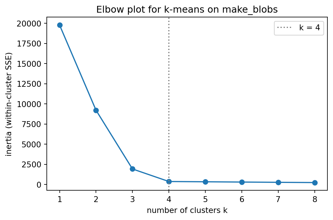
Plot inertia \(J\) against \(k\) and look for the elbow, the value of \(k\) after which additional clusters yield only marginal reductions in inertia. The idea is that real structure produces a sharp initial drop as the major clusters are resolved, followed by diminishing returns once you are merely subdividing genuine clusters. The elbow is intuitive and quick, but it is qualitative: on smooth curves the elbow is ambiguous, and different analysts read it differently.
The plot below sweeps \(k\) from 1 to 8 on the same blob data and traces inertia against \(k\). The sharp drop flattens right at \(k = 4\), the number of clusters the data were generated with.
Code
import matplotlib.pyplot as pltks =range(1, 9)inertias = []for k in ks: model = KMeans(n_clusters=k, init="k-means++", n_init=10, random_state=rng) model.fit(X) inertias.append(model.inertia_)fig, ax = plt.subplots(figsize=(6, 4))ax.plot(list(ks), inertias, marker="o")ax.axvline(4, color="gray", linestyle=":", label="k = 4")ax.set_xlabel("number of clusters k")ax.set_ylabel("inertia (within-cluster SSE)")ax.set_title("Elbow plot for k-means on make_blobs")ax.legend()plt.tight_layout()plt.show()print("Inertia by k:", [round(v, 1) for v in inertias])
The inertia falls steeply from \(k = 1\) through \(k = 4\), then declines only marginally, the classic elbow signature of four genuine clusters.
128.5.2 5.2 The silhouette coefficient
The silhouette method evaluates how well each point fits its cluster relative to the next-best cluster. For a point \(x_i\), let \(a(i)\) be the mean distance to the other points in its own cluster and \(b(i)\) be the mean distance to points in the nearest other cluster. The silhouette of \(x_i\) is
A value near \(1\) means the point is well inside its cluster and far from others; near \(0\) means it sits on a boundary; negative means it is probably misassigned. Averaging \(s(i)\) over all points gives a single score, and the \(k\) that maximizes the mean silhouette is a defensible choice. Unlike the elbow, this criterion is quantitative and accounts for cluster separation, not just compactness, though it costs more to compute because it involves pairwise distances.
128.5.3 5.3 The gap statistic and information criteria
The gap statistic compares the observed inertia at each \(k\) against the inertia expected under a null reference distribution with no clustering, typically uniform data over the bounding region. The best \(k\) is where the observed inertia falls farthest below the null, signaling genuine structure rather than the inertia reduction that any \(k\) would produce on noise. Alternatively, if k-means is recast as a Gaussian mixture with shared spherical covariance, penalized likelihood criteria such as BIC select \(k\) by balancing fit against a parameter-count penalty. In all cases, the statistical signal should be weighed against domain knowledge: the most useful \(k\) is often dictated by how the clusters will be acted on, not by an optimum on a curve.
128.6 6. Assumptions and Limitations
K-means is fast and effective when its assumptions hold, and quietly misleading when they do not. Understanding the implicit model is the difference between a tool and a trap.
128.6.1 6.1 The implicit cluster model
Minimizing within-cluster squared distance with Euclidean geometry implicitly assumes clusters that are roughly spherical, of similar spatial extent, and of comparable population. Each cluster is summarized by a single mean and a decision boundary that is linear; in fact the boundary between any two centroids is the perpendicular bisecting hyperplane between them, so k-means carves space into a Voronoi tessellation. When the true clusters match this picture, k-means recovers them well.
128.6.2 6.2 Where the model breaks
Several common situations violate these assumptions:
Non-convex shapes. Concentric rings or interleaved crescents cannot be separated by Voronoi cells, and k-means will slice them incorrectly. Density-based or spectral methods are appropriate here.
Unequal cluster sizes and densities. Because the objective sums squared distances, a large or diffuse cluster contributes disproportionately, and k-means tends to split it while merging smaller neighbors to keep the total down.
Anisotropic or elongated clusters. Spherical distance penalizes the long axis of a stretched cluster, so a single elongated group may be cut into pieces. A Gaussian mixture with full covariance handles this; k-means does not.
Differing feature scales. Euclidean distance treats all dimensions equally, so a feature measured in large units dominates the assignment. Standardizing features to comparable scale is usually mandatory.
128.6.3 6.3 Sensitivity to outliers and the role of \(k\)
Because centroids are means, a single far-flung outlier can drag a centroid away from the bulk of its cluster, distorting the partition. Robust variants based on medians (k-medoids) resist this at higher computational cost. Finally, k-means always returns exactly \(k\) clusters, even when the data contain none; it will impose structure on uniform noise without complaint. Validation against the criteria of Section 5, and skepticism informed by visualization, are the safeguards.
128.6.4 6.4 Practical checklist
Before trusting a k-means result, confirm that features are scaled, that k-means++ initialization with several restarts was used, that \(k\) was chosen by an explicit criterion rather than by default, and that the recovered clusters have been inspected for the failure modes above. K-means rewards this discipline with a partition that is fast to compute, easy to explain, and faithful to genuinely compact, well-separated structure in the data.
128.7 References
Lloyd, S. P. “Least Squares Quantization in PCM.” IEEE Transactions on Information Theory, 1982. https://doi.org/10.1109/TIT.1982.1056489
MacQueen, J. “Some Methods for Classification and Analysis of Multivariate Observations.” Proceedings of the Fifth Berkeley Symposium on Mathematical Statistics and Probability, 1967. https://projecteuclid.org/euclid.bsmsp/1200512992
Arthur, D. and Vassilvitskii, S. “k-means++: The Advantages of Careful Seeding.” Proceedings of the ACM-SIAM Symposium on Discrete Algorithms (SODA), 2007. https://dl.acm.org/doi/10.5555/1283383.1283494
Bahmani, B., Moseley, B., Vattani, A., Kumar, R., and Vassilvitskii, S. “Scalable k-means++.” Proceedings of the VLDB Endowment, 2012. https://doi.org/10.14778/2180912.2180915
Arthur, D. and Vassilvitskii, S. “How Slow is the k-means Method?” Proceedings of the Symposium on Computational Geometry (SoCG), 2006. https://doi.org/10.1145/1137856.1137880
Aloise, D., Deshpande, A., Hansen, P., and Popat, P. “NP-hardness of Euclidean Sum-of-Squares Clustering.” Machine Learning, 2009. https://doi.org/10.1007/s10994-009-5103-0
Rousseeuw, P. J. “Silhouettes: A Graphical Aid to the Interpretation and Validation of Cluster Analysis.” Journal of Computational and Applied Mathematics, 1987. https://doi.org/10.1016/0377-0427(87)90125-7
Tibshirani, R., Walther, G., and Hastie, T. “Estimating the Number of Clusters in a Data Set via the Gap Statistic.” Journal of the Royal Statistical Society: Series B, 2001. https://doi.org/10.1111/1467-9868.00293
Pedregosa, F. et al. “Scikit-learn: Machine Learning in Python.” Journal of Machine Learning Research, 2011. https://jmlr.org/papers/v12/pedregosa11a.html
Source Code
# K-Means ClusteringK-means is the most widely used clustering algorithm in practice, and for good reason: it is simple to state, fast to run, and yields a partition that is easy to interpret. Beneath that simplicity lies a rich optimization problem with subtle geometry. This chapter develops the objective that k-means minimizes, the iterative procedure (Lloyd's algorithm) that descends on it, the seeding scheme (k-means++) that makes the procedure reliable, and the theory around convergence, model selection, and the assumptions the method silently encodes. The goal is to leave you able to apply k-means with judgment rather than as a black box.## 1. The Clustering Objective### 1.1 Problem statementWe are given $n$ data points $x_1, \dots, x_n \in \mathbb{R}^d$ and a target number of clusters $k$. We seek a partition of the points into $k$ disjoint sets $C_1, \dots, C_k$ together with a set of representatives, called centroids, $\mu_1, \dots, \mu_k \in \mathbb{R}^d$. K-means defines the quality of such an assignment through the within-cluster sum of squares, also called inertia or distortion:$$J(C, \mu) = \sum_{j=1}^{k} \sum_{x_i \in C_j} \lVert x_i - \mu_j \rVert_2^2 .$$The objective rewards partitions in which every point sits close, in squared Euclidean distance, to the centroid of its assigned cluster. Minimizing $J$ over both the assignment $C$ and the centroids $\mu$ is the k-means problem.### 1.2 Why squared Euclidean distanceThe choice of squared $\ell_2$ distance is not cosmetic; it is what makes the centroid the optimal representative. Fix a cluster $C_j$ and ask which point $\mu_j$ minimizes $\sum_{x_i \in C_j} \lVert x_i - \mu_j \rVert_2^2$. Setting the gradient to zero gives$$\sum_{x_i \in C_j} 2 (\mu_j - x_i) = 0 \quad \Longrightarrow \quad \mu_j = \frac{1}{|C_j|} \sum_{x_i \in C_j} x_i .$$The minimizer is exactly the arithmetic mean, which is where the name k-means comes from. If we instead used the $\ell_1$ distance, the optimal representative would be the coordinatewise median, giving the k-medians algorithm; if we restricted representatives to be actual data points, we would get k-medoids. The squared norm also yields a useful identity: the total inertia equals the sum over clusters of $|C_j|$ times the variance within $C_j$, so k-means can be read as variance minimization.### 1.3 Computational hardnessDespite its simple form, exactly minimizing $J$ is NP-hard. The difficulty holds even for $k = 2$ clusters in general dimension, and separately for fixed dimension $d = 2$ with general $k$. There are roughly $k^n / k!$ ways to partition $n$ points into $k$ nonempty groups, an astronomical search space. We therefore do not solve k-means exactly. We rely on local-search heuristics that find good partitions quickly, accepting that they may not reach the global optimum. Lloyd's algorithm is the canonical such heuristic.## 2. Lloyd's Algorithm### 2.1 Coordinate descent on two variablesThe objective $J(C, \mu)$ depends on two groups of variables: the discrete assignments $C$ and the continuous centroids $\mu$. Lloyd's algorithm performs alternating minimization, optimizing one group while holding the other fixed.Assignment step. With centroids fixed, the objective decomposes across points: each $x_i$ contributes $\min_j \lVert x_i - \mu_j \rVert^2$ to the total if assigned optimally. The best move is to assign every point to its nearest centroid:$$c_i = \arg\min_{j \in \{1, \dots, k\}} \lVert x_i - \mu_j \rVert_2^2 .$$Update step. With assignments fixed, we showed in Section 1.2 that the optimal centroid of each cluster is the mean of its members:$$\mu_j = \frac{1}{|C_j|} \sum_{x_i \in C_j} x_i .$$We iterate these two steps until the assignments stop changing.```textinitialize centroids mu_1 ... mu_krepeat: # assignment step for each point x_i: c_i = index of nearest centroid # update step for each cluster j: mu_j = mean of points assigned to juntil assignments unchanged```We can run this on synthetic data. We generate four well-separated blobs and let scikit-learn's k-means (which implements Lloyd's algorithm) partition them, then report the recovered cluster sizes, the final inertia, and how many iterations convergence took.```{python}import numpy as npfrom sklearn.datasets import make_blobsfrom sklearn.cluster import KMeansrng =42X, y_true = make_blobs(n_samples=300, centers=4, cluster_std=0.80, random_state=rng)km = KMeans(n_clusters=4, init="k-means++", n_init=10, random_state=rng)labels = km.fit_predict(X)counts = np.bincount(labels)print("Cluster sizes:", counts)print("Final inertia: {:.2f}".format(km.inertia_))print("Iterations to converge:", km.n_iter_)```The four true clusters are each recovered with their full membership, and the algorithm settles in only a few iterations.### 2.2 Monotone descent and finite terminationEach step weakly decreases $J$. The assignment step lowers (or holds) every point's contribution because reassigning to the nearest centroid can only shrink its squared distance. The update step lowers (or holds) each cluster's contribution because the mean is the unique minimizer of within-cluster squared distance. Therefore the sequence of objective values is nonincreasing.Because there are only finitely many distinct assignments (at most $k^n$), and the objective strictly decreases whenever an assignment changes, the algorithm cannot cycle and must terminate after a finite number of iterations. In practice it usually converges in a few dozen iterations or fewer, though contrived inputs can force a number of iterations exponential in $n$. The smoothed complexity is polynomial, which explains why the worst case almost never appears on real data.### 2.3 Cost per iterationA single iteration computes the distance from each of $n$ points to each of $k$ centroids in $d$ dimensions, costing $O(nkd)$ time. The update step is also $O(nd)$ since it is one pass to accumulate sums. With $T$ iterations the total is $O(nkdT)$, linear in the number of points. This scalability is the practical reason k-means dominates: it handles large $n$ where most clustering methods, which need pairwise distances at $O(n^2)$ cost, cannot.### 2.4 Empty clustersA subtlety: the update step assumes every cluster is nonempty. If a centroid ends up with no assigned points, its mean is undefined. Standard implementations handle this by reseeding the empty centroid, for instance to the point that is currently farthest from its assigned centroid, which both repairs the partition and tends to reduce the objective.## 3. The k-means++ Initialization### 3.1 Why initialization mattersLloyd's algorithm converges only to a local minimum, and which local minimum it reaches depends entirely on the starting centroids. Naive initialization, sampling $k$ points uniformly at random, frequently places two seeds in the same dense region and none in another, producing a poor partition that no amount of iterating can escape. The standard remedy is to run Lloyd from many random starts and keep the best, but that wastes computation and still offers no guarantee.### 3.2 The seeding procedureK-means++ replaces uniform seeding with a careful, adaptive sampling scheme that spreads the initial centroids out. It chooses the first center uniformly at random, then chooses each subsequent center with probability proportional to its squared distance from the nearest already-chosen center.```textchoose c_1 uniformly at random from the datafor j = 2 ... k: for each point x_i: D(x_i) = distance to nearest already-chosen center choose c_j = x_i with probability proportional to D(x_i)^2run Lloyd's algorithm from these k centers```The intuition is that a point far from all current centers is precisely a point that the current seeding represents poorly, so it is a strong candidate to anchor a new cluster. The squared weighting biases selection toward such points while retaining randomness, which prevents the procedure from always grabbing outliers.### 3.3 The approximation guaranteeThe reason k-means++ is more than a heuristic is its provable guarantee. Let $J^\star$ be the optimal value of the k-means objective. The expected cost of the partition obtained right after k-means++ seeding, before any Lloyd iterations, satisfies$$\mathbb{E}[J] \le 8 (\ln k + 2) \, J^\star .$$The seeding alone is $O(\log k)$-competitive with the global optimum in expectation. Running Lloyd's algorithm afterward only improves on this. The practical effect is dramatic: k-means++ typically reaches a lower final objective, converges in fewer iterations, and exhibits far less variance across random seeds than uniform initialization. It is the default initializer in essentially every mature k-means library, and it is what you should use unless you have a specific reason not to.### 3.4 Scalable variantsThe sequential nature of k-means++ requires $k$ passes over the data, which becomes a bottleneck at very large scale. The variant k-means|| (k-means parallel) oversamples several candidate centers per round across a constant number of rounds, then reclusters the candidate set down to $k$ centers. It retains a similar approximation quality while parallelizing cleanly across a distributed dataset.## 4. Convergence and Local Minima### 4.1 What convergence does and does not promiseLloyd's algorithm converges in the sense that the objective stops decreasing and the assignments stabilize. It does not promise that the resulting partition is globally optimal, or even close. The fixed points of the iteration are the partitions where no point wants to move and no centroid wants to shift; these are local minima of $J$, and there can be many of them with widely differing quality.### 4.2 A worked failure caseConsider four well-separated clusters arranged at the corners of a square, with $k = 4$. If initialization places two centroids inside the top-left cluster and the remaining two split between the bottom corners, Lloyd's algorithm will happily converge: the two top-left centroids divide that one true cluster between them, while one of the bottom centroids is stretched to cover two true clusters at once. Every point is assigned to its nearest centroid and every centroid is the mean of its members, so the fixed-point conditions hold. The objective is far above optimal, yet no local step can improve it. This is exactly the configuration that good initialization is designed to avoid.### 4.3 Practical mitigationsThree tactics address local minima. First, use k-means++ seeding, which makes such pathological starts unlikely. Second, run multiple independent restarts (the `n_init` parameter in common libraries) and keep the partition with the lowest inertia; with k-means++ seeding even a handful of restarts is usually enough. Third, standardize or otherwise scale features before clustering so that no dimension dominates the distance and distorts the geometry the algorithm sees. These are cheap, and skipping them is the most common cause of disappointing k-means results.## 5. Choosing the Number of ClustersK-means requires $k$ as an input, yet the right $k$ is rarely known in advance. Worse, the objective $J$ cannot be used directly to choose $k$, because $J$ is monotonically nonincreasing in $k$: adding clusters always lets points sit closer to a centroid, and at $k = n$ the inertia reaches zero. We need criteria that trade fit against complexity.### 5.1 The elbow methodPlot inertia $J$ against $k$ and look for the elbow, the value of $k$ after which additional clusters yield only marginal reductions in inertia. The idea is that real structure produces a sharp initial drop as the major clusters are resolved, followed by diminishing returns once you are merely subdividing genuine clusters. The elbow is intuitive and quick, but it is qualitative: on smooth curves the elbow is ambiguous, and different analysts read it differently.The plot below sweeps $k$ from 1 to 8 on the same blob data and traces inertia against $k$. The sharp drop flattens right at $k = 4$, the number of clusters the data were generated with.```{python}import matplotlib.pyplot as pltks =range(1, 9)inertias = []for k in ks: model = KMeans(n_clusters=k, init="k-means++", n_init=10, random_state=rng) model.fit(X) inertias.append(model.inertia_)fig, ax = plt.subplots(figsize=(6, 4))ax.plot(list(ks), inertias, marker="o")ax.axvline(4, color="gray", linestyle=":", label="k = 4")ax.set_xlabel("number of clusters k")ax.set_ylabel("inertia (within-cluster SSE)")ax.set_title("Elbow plot for k-means on make_blobs")ax.legend()plt.tight_layout()plt.show()print("Inertia by k:", [round(v, 1) for v in inertias])```The inertia falls steeply from $k = 1$ through $k = 4$, then declines only marginally, the classic elbow signature of four genuine clusters.### 5.2 The silhouette coefficientThe silhouette method evaluates how well each point fits its cluster relative to the next-best cluster. For a point $x_i$, let $a(i)$ be the mean distance to the other points in its own cluster and $b(i)$ be the mean distance to points in the nearest other cluster. The silhouette of $x_i$ is$$s(i) = \frac{b(i) - a(i)}{\max\{a(i),\, b(i)\}} \in [-1, 1] .$$A value near $1$ means the point is well inside its cluster and far from others; near $0$ means it sits on a boundary; negative means it is probably misassigned. Averaging $s(i)$ over all points gives a single score, and the $k$ that maximizes the mean silhouette is a defensible choice. Unlike the elbow, this criterion is quantitative and accounts for cluster separation, not just compactness, though it costs more to compute because it involves pairwise distances.### 5.3 The gap statistic and information criteriaThe gap statistic compares the observed inertia at each $k$ against the inertia expected under a null reference distribution with no clustering, typically uniform data over the bounding region. The best $k$ is where the observed inertia falls farthest below the null, signaling genuine structure rather than the inertia reduction that any $k$ would produce on noise. Alternatively, if k-means is recast as a Gaussian mixture with shared spherical covariance, penalized likelihood criteria such as BIC select $k$ by balancing fit against a parameter-count penalty. In all cases, the statistical signal should be weighed against domain knowledge: the most useful $k$ is often dictated by how the clusters will be acted on, not by an optimum on a curve.## 6. Assumptions and LimitationsK-means is fast and effective when its assumptions hold, and quietly misleading when they do not. Understanding the implicit model is the difference between a tool and a trap.### 6.1 The implicit cluster modelMinimizing within-cluster squared distance with Euclidean geometry implicitly assumes clusters that are roughly spherical, of similar spatial extent, and of comparable population. Each cluster is summarized by a single mean and a decision boundary that is linear; in fact the boundary between any two centroids is the perpendicular bisecting hyperplane between them, so k-means carves space into a Voronoi tessellation. When the true clusters match this picture, k-means recovers them well.### 6.2 Where the model breaksSeveral common situations violate these assumptions:- Non-convex shapes. Concentric rings or interleaved crescents cannot be separated by Voronoi cells, and k-means will slice them incorrectly. Density-based or spectral methods are appropriate here.- Unequal cluster sizes and densities. Because the objective sums squared distances, a large or diffuse cluster contributes disproportionately, and k-means tends to split it while merging smaller neighbors to keep the total down.- Anisotropic or elongated clusters. Spherical distance penalizes the long axis of a stretched cluster, so a single elongated group may be cut into pieces. A Gaussian mixture with full covariance handles this; k-means does not.- Differing feature scales. Euclidean distance treats all dimensions equally, so a feature measured in large units dominates the assignment. Standardizing features to comparable scale is usually mandatory.### 6.3 Sensitivity to outliers and the role of $k$Because centroids are means, a single far-flung outlier can drag a centroid away from the bulk of its cluster, distorting the partition. Robust variants based on medians (k-medoids) resist this at higher computational cost. Finally, k-means always returns exactly $k$ clusters, even when the data contain none; it will impose structure on uniform noise without complaint. Validation against the criteria of Section 5, and skepticism informed by visualization, are the safeguards.### 6.4 Practical checklistBefore trusting a k-means result, confirm that features are scaled, that k-means++ initialization with several restarts was used, that $k$ was chosen by an explicit criterion rather than by default, and that the recovered clusters have been inspected for the failure modes above. K-means rewards this discipline with a partition that is fast to compute, easy to explain, and faithful to genuinely compact, well-separated structure in the data.## References1. Lloyd, S. P. "Least Squares Quantization in PCM." IEEE Transactions on Information Theory, 1982. https://doi.org/10.1109/TIT.1982.10564892. MacQueen, J. "Some Methods for Classification and Analysis of Multivariate Observations." Proceedings of the Fifth Berkeley Symposium on Mathematical Statistics and Probability, 1967. https://projecteuclid.org/euclid.bsmsp/12005129923. Arthur, D. and Vassilvitskii, S. "k-means++: The Advantages of Careful Seeding." Proceedings of the ACM-SIAM Symposium on Discrete Algorithms (SODA), 2007. https://dl.acm.org/doi/10.5555/1283383.12834944. Bahmani, B., Moseley, B., Vattani, A., Kumar, R., and Vassilvitskii, S. "Scalable k-means++." Proceedings of the VLDB Endowment, 2012. https://doi.org/10.14778/2180912.21809155. Arthur, D. and Vassilvitskii, S. "How Slow is the k-means Method?" Proceedings of the Symposium on Computational Geometry (SoCG), 2006. https://doi.org/10.1145/1137856.11378806. Aloise, D., Deshpande, A., Hansen, P., and Popat, P. "NP-hardness of Euclidean Sum-of-Squares Clustering." Machine Learning, 2009. https://doi.org/10.1007/s10994-009-5103-07. Rousseeuw, P. J. "Silhouettes: A Graphical Aid to the Interpretation and Validation of Cluster Analysis." Journal of Computational and Applied Mathematics, 1987. https://doi.org/10.1016/0377-0427(87)90125-78. Tibshirani, R., Walther, G., and Hastie, T. "Estimating the Number of Clusters in a Data Set via the Gap Statistic." Journal of the Royal Statistical Society: Series B, 2001. https://doi.org/10.1111/1467-9868.002939. Pedregosa, F. et al. "Scikit-learn: Machine Learning in Python." Journal of Machine Learning Research, 2011. https://jmlr.org/papers/v12/pedregosa11a.html