Backpropagation is the algorithm that makes deep learning practical. It computes the gradient of a scalar loss with respect to every parameter in a network using a single backward sweep whose cost is comparable to one forward evaluation. Modern frameworks hide this machinery behind automatic differentiation, but the abstraction leaks the moment a gradient comes back wrong, a loss refuses to descend, or a custom layer needs a hand written derivative. This chapter builds a small multilayer perceptron in NumPy, derives the backward pass term by term, verifies it with numerical gradient checking, and catalogs the bugs that most often defeat a first implementation.
193.1 1. The Computational Setting
Consider a feedforward network that maps an input batch \(X \in \mathbb{R}^{N \times d_0}\) to predictions, where \(N\) is the batch size and \(d_0\) the input dimension. We use a two layer architecture for concreteness, though the pattern generalizes to any depth. The forward computation is a chain of affine transforms interleaved with nonlinearities:
Here \(W_1 \in \mathbb{R}^{d_0 \times d_1}\) and \(W_2 \in \mathbb{R}^{d_1 \times C}\) are weight matrices, \(b_1\) and \(b_2\) are bias vectors broadcast across the batch, \(\phi\) is an elementwise activation such as ReLU, and \(C\) is the number of classes. The training objective is the average cross entropy over the batch:
\[
L = -\frac{1}{N} \sum_{i=1}^{N} \sum_{c=1}^{C} Y_{ic} \log \hat{Y}_{ic},
\]
where \(Y\) is the one hot label matrix. Our goal is to compute \(\partial L / \partial W_1\), \(\partial L / \partial b_1\), \(\partial L / \partial W_2\), and \(\partial L / \partial b_2\) so that a gradient descent step can update the parameters.
193.1.1 1.1 Why a Backward Pass
A naive approach would perturb each parameter, rerun the forward pass, and estimate the derivative by finite differences. For a network with \(P\) parameters this costs \(O(P)\) forward passes per gradient, which is hopeless when \(P\) runs into the millions. Backpropagation instead exploits the chain rule and the structure of the computational graph to obtain all \(P\) partial derivatives in a single backward traversal whose cost is a small constant multiple of one forward pass. The key insight is reuse: the gradient flowing into a node is computed once and reused for every parameter that feeds it.
193.2 2. The Forward Cache
The backward pass needs intermediate quantities from the forward pass. The product rule for a matrix multiply \(Z = A W\) produces \(\partial L / \partial W = A^\top (\partial L / \partial Z)\), so we must retain \(A\). Likewise the derivative of a ReLU depends on the sign of its preinput \(Z_1\). The discipline of storing exactly these quantities is the forward cache, and getting its contents right is half the battle.
A useful rule of thumb: cache every tensor that appears on the right hand side of a gradient expression. In practice this means the layer inputs and the preactivations. We do not need to cache the loss itself, and we usually do not need the final activation \(\hat{Y}\) separately because the softmax and cross entropy combine into a simple gradient, discussed below.
Code
import numpy as npdef relu(z):return np.maximum(0.0, z)def softmax(z): z = z - z.max(axis=1, keepdims=True) # subtract max for stability e = np.exp(z)return e / e.sum(axis=1, keepdims=True)class MLP:def__init__(self, d0, d1, C, seed=0): rng = np.random.default_rng(seed)# He initialization for the ReLU layer, Xavier-like for the outputself.W1 = rng.standard_normal((d0, d1)) * np.sqrt(2.0/ d0)self.b1 = np.zeros(d1)self.W2 = rng.standard_normal((d1, C)) * np.sqrt(1.0/ d1)self.b2 = np.zeros(C)self.cache = {}def forward(self, X): Z1 = X @self.W1 +self.b1 A1 = relu(Z1) Z2 = A1 @self.W2 +self.b2 Yhat = softmax(Z2)# Store everything the backward pass will consume.self.cache = {"X": X, "Z1": Z1, "A1": A1, "Yhat": Yhat}return Yhat# Quick check: softmax rows form valid probability distributions._demo = MLP(d0=4, d1=6, C=3)_probs = _demo.forward(np.zeros((5, 4)))print("forward output shape:", _probs.shape)print("each row sums to one:", np.allclose(_probs.sum(axis=1), 1.0))
forward output shape: (5, 3)
each row sums to one: True
Notice that the forward method has a side effect: it populates self.cache. This couples a forward call to a subsequent backward call, which is a deliberate design choice for clarity. Production code often makes the cache explicit by passing it as a return value, which avoids subtle bugs when two forward passes happen before a backward pass.
193.3 3. The Backward Pass
We now derive each gradient. Throughout, we write \(\delta_k = \partial L / \partial Z_k\) for the gradient of the loss with respect to a preactivation. These delta terms are the currency of backpropagation, and once a delta is known the parameter gradients at that layer follow mechanically.
193.3.1 3.1 The Softmax Cross Entropy Gradient
The single most useful identity in classification networks is that the gradient of cross entropy with respect to the softmax logits collapses to a difference. If \(\hat{Y} = \text{softmax}(Z_2)\) and \(L\) is the averaged cross entropy, then
This compact form arises because the Jacobian of the softmax and the gradient of the logarithm cancel almost entirely. Computing the two derivatives separately and multiplying their Jacobians is numerically fragile and wasteful, so we treat the softmax and cross entropy as a fused operation. The factor \(1/N\) comes from averaging the loss over the batch.
193.3.2 3.2 Output Layer Parameters
Given \(\delta_2\), the affine transform \(Z_2 = A_1 W_2 + b_2\) yields the gradients by applying the multivariable chain rule:
The bias gradient is a sum over the batch dimension because the same bias vector is broadcast to every example, so its contributions accumulate. The gradient \(\partial L / \partial A_1\) is what we propagate backward into the hidden layer.
193.3.3 3.3 Hidden Layer Parameters
The ReLU sits between \(Z_1\) and \(A_1\), and its local derivative is the indicator that the preactivation was positive:
This symmetry is the heart of backpropagation. Every affine layer has the same three gradient formulas, differing only in which cached input and which incoming delta they use. The algorithm is therefore a loop over layers, not a special case per layer.
Code
def backward(self, Y): X =self.cache["X"] Z1 =self.cache["Z1"] A1 =self.cache["A1"] Yhat =self.cache["Yhat"] N = X.shape[0]# Fused softmax + cross-entropy gradient at the logits. dZ2 = (Yhat - Y) / N # (N, C)# Output affine layer. dW2 = A1.T @ dZ2 # (d1, C) db2 = dZ2.sum(axis=0) # (C,) dA1 = dZ2 @self.W2.T # (N, d1)# ReLU backward: gate the upstream gradient by the forward sign. dZ1 = dA1 * (Z1 >0) # (N, d1)# Input affine layer. dW1 = X.T @ dZ1 # (d0, d1) db1 = dZ1.sum(axis=0) # (d1,)return {"W1": dW1, "b1": db1, "W2": dW2, "b2": db2}# Attach the backward pass to the class defined above.MLP.backward = backward# Sanity check: parameter gradients match their parameter shapes._demo.forward(np.zeros((5, 4)))_g = _demo.backward(np.eye(3)[[0, 1, 2, 0, 1]])print("gradient shapes match parameters:",all(_g[n].shape ==getattr(_demo, n).shape for n in ("W1", "b1", "W2", "b2")))
gradient shapes match parameters: True
193.3.4 3.4 Putting It Together
A single training step combines a forward pass, a loss evaluation, a backward pass, and a parameter update. The loss function is kept separate so the gradient check in the next section can call it independently.
Code
def cross_entropy(Yhat, Y): N = Yhat.shape[0] eps =1e-12# guard against log(0)return-np.sum(Y * np.log(Yhat + eps)) / Ndef sgd_step(model, X, Y, lr=0.1): Yhat = model.forward(X) loss = cross_entropy(Yhat, Y) grads = model.backward(Y)for name in ("W1", "b1", "W2", "b2"):getattr(model, name)[...] -= lr * grads[name]return loss
The in place update getattr(model, name)[...] -= ... modifies the parameter array without rebinding the attribute, which keeps the cache and any external references valid. Rebinding with a plain assignment would also work here but is a common source of confusion when parameters are shared.
193.4 4. Gradient Checking
An analytic gradient is only trustworthy once it has been validated against a numerical estimate. The central difference approximation of a partial derivative is
where \(e_j\) is the unit vector along parameter \(\theta_j\). The central difference has error \(O(\epsilon^2)\), far better than the one sided \(O(\epsilon)\) alternative, and a value of \(\epsilon \approx 10^{-5}\) usually balances truncation error against floating point round off. We compare analytic and numerical gradients with the relative error
with a small \(\eta\) to avoid dividing by zero. A relative error below \(10^{-7}\) is excellent, below \(10^{-5}\) is generally acceptable for a network using smooth activations, and anything above \(10^{-3}\) signals a bug.
Several practical points govern a reliable check. Run it on a tiny network with a handful of units, because the procedure costs two forward passes per parameter and is far too slow for full models. Use double precision throughout, since the small \(\epsilon\) perturbations are lost in the noise of float32. Avoid checking near nondifferentiable points: ReLU has a kink at zero where the numerical and analytic gradients legitimately disagree, so if a preactivation sits very close to zero, nudge the inputs or switch temporarily to a smooth activation such as tanh for the duration of the check. Finally, check one parameter group at a time so that a failure localizes the bug to a specific layer.
193.5 5. Common Bugs
The arithmetic of backpropagation is simple, but the bookkeeping is unforgiving. The following failures recur often enough to deserve a checklist.
193.5.1 5.1 Transpose and Shape Errors
The most frequent mistake is multiplying matrices in the wrong order or forgetting a transpose. The discipline that prevents this is dimensional analysis: a parameter gradient must have exactly the same shape as the parameter. Since \(W_1\) is \(d_0 \times d_1\), its gradient must be \(d_0 \times d_1\), which forces the product \(X^\top \delta_1\) rather than \(\delta_1^\top X\) or \(X \delta_1\). When a shape does not line up, NumPy will often broadcast silently instead of raising an error, producing a wrong gradient that still runs. Asserting expected shapes during development catches these immediately.
193.5.2 5.2 Forgetting the Batch Average
If the loss divides by \(N\) but the gradient does not, every parameter update is scaled by a factor of \(N\), which manifests as a learning rate that is mysteriously too large. The cleanest fix is to fold the \(1/N\) into \(\delta_2\) once, as we did, so that it propagates automatically to every downstream gradient. Mixing a summed loss with an averaged gradient, or vice versa, is a classic source of divergence.
193.5.3 5.3 Cache Staleness
When the backward pass reads a cache that a later forward pass has overwritten, gradients correspond to the wrong inputs. This happens when evaluation and training share a model instance, or when a gradient check calls forward repeatedly. The grad check above is careful to call model.forward(X) immediately before reading the analytic gradient so that the cache matches. Making the cache an explicit argument rather than instance state eliminates this class of bug entirely.
193.5.4 5.4 Numerical Instability in Softmax
Computing \(\exp(Z_2)\) without subtracting the row maximum overflows to infinity for moderately large logits, and the subsequent division yields NaN. The stabilized softmax in our forward pass subtracts the per row maximum, which leaves the result mathematically unchanged because softmax is invariant to a constant shift in its inputs. Similarly, \(\log(0)\) in the cross entropy produces negative infinity, which the small \(\epsilon\) guard prevents. These guards do not change the analytic gradient, since the fused softmax cross entropy derivative never evaluates the unstable intermediate.
193.5.5 5.5 The ReLU Gating Mistake
A subtle error is gating the wrong tensor in the ReLU backward step. The mask must come from the cached preactivation \(Z_1\), not from the activation \(A_1\) or from the incoming gradient. Using \(A_1 > 0\) happens to give the same mask for ReLU because the activation is zero exactly where the preactivation is nonpositive, but the equivalence breaks for activations like leaky ReLU or for any function whose output sign differs from its input sign. Always derive the mask from the quantity the activation actually differentiates against.
193.5.6 5.6 In Place Mutation of Cached Tensors
If the backward pass modifies a cached array in place, for example by writing dZ1 *= mask onto a view of A1, a later read of the cache returns corrupted data. NumPy views make this easy to do by accident. The safe habit is to allocate new arrays for gradients and to treat cached tensors as read only.
193.6 6. Verifying the Whole System
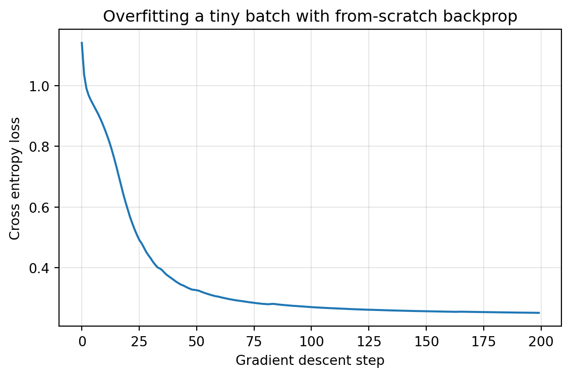
A final integration test runs the gradient check across all four parameter groups and confirms that a few steps of gradient descent reduce the loss on a synthetic problem. If every relative error is small and the loss falls monotonically on a tiny overfit set, the implementation is almost certainly correct.
Code
import matplotlib.pyplot as plt# Synthetic sanity check.rng = np.random.default_rng(1)X = rng.standard_normal((8, 5))labels = rng.integers(0, 3, size=8)Y = np.eye(3)[labels]model = MLP(d0=5, d1=4, C=3)print("Gradient check (relative error per parameter group):")for name in ("W1", "b1", "W2", "b2"):print(f" {name:>3} rel error = {grad_check(model, X, Y, name):.2e}")# Overfit a tiny batch; loss should march toward zero.losses = []for step inrange(200): losses.append(sgd_step(model, X, Y, lr=0.5))print(f"\ninitial loss: {losses[0]:.4f} final loss: {losses[-1]:.4f}")fig, ax = plt.subplots(figsize=(6, 4))ax.plot(losses, color="#1f77b4")ax.set_xlabel("Gradient descent step")ax.set_ylabel("Cross entropy loss")ax.set_title("Overfitting a tiny batch with from-scratch backprop")ax.grid(True, alpha=0.3)fig.tight_layout()plt.show()
The ability to overfit a small batch to near zero loss is the single most informative smoke test for a network and its gradients. A correct implementation drives the loss down quickly; a network that plateaus high almost always has a gradient bug, a broken cache, or a learning rate problem, and the gradient check above will usually pinpoint which.
193.7 7. Generalizing the Pattern
The two layer example exposes the recursive structure that scales to arbitrary depth. Each layer needs three things: a forward function that produces an output and caches its inputs, a backward function that converts an incoming gradient into a parameter gradient and an outgoing gradient, and a record of the order in which layers were applied. The backward pass then walks the layers in reverse, threading the delta from one to the next. This is precisely the abstraction that reverse mode automatic differentiation generalizes, replacing the hand written per layer rules with a graph of primitive operations each carrying its own local derivative. Understanding the manual version makes the automatic version legible rather than magical, and it equips you to debug the cases where the framework’s gradient is not the one you expected.
193.8 References
Rumelhart, D. E., Hinton, G. E., and Williams, R. J. “Learning representations by back-propagating errors.” Nature, 1986. https://www.nature.com/articles/323533a0
Goodfellow, I., Bengio, Y., and Courville, A. Deep Learning, Chapter 6. MIT Press, 2016. https://www.deeplearningbook.org/
Karpathy, A. “CS231n: Optimization and Backpropagation lecture notes.” Stanford University. https://cs231n.github.io/optimization-2/
Nielsen, M. “How the backpropagation algorithm works.” Neural Networks and Deep Learning, 2015. http://neuralnetworksanddeeplearning.com/chap2.html
Baydin, A. G., Pearlmutter, B. A., Radul, A. A., and Siskind, J. M. “Automatic differentiation in machine learning: a survey.” Journal of Machine Learning Research, 2018. https://jmlr.org/papers/v18/17-468.html
He, K., Zhang, X., Ren, S., and Sun, J. “Delving deep into rectifiers: Surpassing human-level performance on ImageNet classification.” ICCV, 2015. https://arxiv.org/abs/1502.01852
Source Code
# Implementing Backpropagation from ScratchBackpropagation is the algorithm that makes deep learning practical. It computes the gradient of a scalar loss with respect to every parameter in a network using a single backward sweep whose cost is comparable to one forward evaluation. Modern frameworks hide this machinery behind automatic differentiation, but the abstraction leaks the moment a gradient comes back wrong, a loss refuses to descend, or a custom layer needs a hand written derivative. This chapter builds a small multilayer perceptron in NumPy, derives the backward pass term by term, verifies it with numerical gradient checking, and catalogs the bugs that most often defeat a first implementation.## 1. The Computational SettingConsider a feedforward network that maps an input batch $X \in \mathbb{R}^{N \times d_0}$ to predictions, where $N$ is the batch size and $d_0$ the input dimension. We use a two layer architecture for concreteness, though the pattern generalizes to any depth. The forward computation is a chain of affine transforms interleaved with nonlinearities:$$Z_1 = X W_1 + b_1, \qquad A_1 = \phi(Z_1), \qquad Z_2 = A_1 W_2 + b_2, \qquad \hat{Y} = \text{softmax}(Z_2).$$Here $W_1 \in \mathbb{R}^{d_0 \times d_1}$ and $W_2 \in \mathbb{R}^{d_1 \times C}$ are weight matrices, $b_1$ and $b_2$ are bias vectors broadcast across the batch, $\phi$ is an elementwise activation such as ReLU, and $C$ is the number of classes. The training objective is the average cross entropy over the batch:$$L = -\frac{1}{N} \sum_{i=1}^{N} \sum_{c=1}^{C} Y_{ic} \log \hat{Y}_{ic},$$where $Y$ is the one hot label matrix. Our goal is to compute $\partial L / \partial W_1$, $\partial L / \partial b_1$, $\partial L / \partial W_2$, and $\partial L / \partial b_2$ so that a gradient descent step can update the parameters.### 1.1 Why a Backward PassA naive approach would perturb each parameter, rerun the forward pass, and estimate the derivative by finite differences. For a network with $P$ parameters this costs $O(P)$ forward passes per gradient, which is hopeless when $P$ runs into the millions. Backpropagation instead exploits the chain rule and the structure of the computational graph to obtain all $P$ partial derivatives in a single backward traversal whose cost is a small constant multiple of one forward pass. The key insight is reuse: the gradient flowing into a node is computed once and reused for every parameter that feeds it.## 2. The Forward CacheThe backward pass needs intermediate quantities from the forward pass. The product rule for a matrix multiply $Z = A W$ produces $\partial L / \partial W = A^\top (\partial L / \partial Z)$, so we must retain $A$. Likewise the derivative of a ReLU depends on the sign of its preinput $Z_1$. The discipline of storing exactly these quantities is the **forward cache**, and getting its contents right is half the battle.A useful rule of thumb: cache every tensor that appears on the right hand side of a gradient expression. In practice this means the layer inputs and the preactivations. We do not need to cache the loss itself, and we usually do not need the final activation $\hat{Y}$ separately because the softmax and cross entropy combine into a simple gradient, discussed below.```{python}import numpy as npdef relu(z):return np.maximum(0.0, z)def softmax(z): z = z - z.max(axis=1, keepdims=True) # subtract max for stability e = np.exp(z)return e / e.sum(axis=1, keepdims=True)class MLP:def__init__(self, d0, d1, C, seed=0): rng = np.random.default_rng(seed)# He initialization for the ReLU layer, Xavier-like for the outputself.W1 = rng.standard_normal((d0, d1)) * np.sqrt(2.0/ d0)self.b1 = np.zeros(d1)self.W2 = rng.standard_normal((d1, C)) * np.sqrt(1.0/ d1)self.b2 = np.zeros(C)self.cache = {}def forward(self, X): Z1 = X @self.W1 +self.b1 A1 = relu(Z1) Z2 = A1 @self.W2 +self.b2 Yhat = softmax(Z2)# Store everything the backward pass will consume.self.cache = {"X": X, "Z1": Z1, "A1": A1, "Yhat": Yhat}return Yhat# Quick check: softmax rows form valid probability distributions._demo = MLP(d0=4, d1=6, C=3)_probs = _demo.forward(np.zeros((5, 4)))print("forward output shape:", _probs.shape)print("each row sums to one:", np.allclose(_probs.sum(axis=1), 1.0))```Notice that the forward method has a side effect: it populates `self.cache`. This couples a forward call to a subsequent backward call, which is a deliberate design choice for clarity. Production code often makes the cache explicit by passing it as a return value, which avoids subtle bugs when two forward passes happen before a backward pass.## 3. The Backward PassWe now derive each gradient. Throughout, we write $\delta_k = \partial L / \partial Z_k$ for the gradient of the loss with respect to a preactivation. These delta terms are the currency of backpropagation, and once a delta is known the parameter gradients at that layer follow mechanically.### 3.1 The Softmax Cross Entropy GradientThe single most useful identity in classification networks is that the gradient of cross entropy with respect to the softmax logits collapses to a difference. If $\hat{Y} = \text{softmax}(Z_2)$ and $L$ is the averaged cross entropy, then$$\delta_2 = \frac{\partial L}{\partial Z_2} = \frac{1}{N}\left(\hat{Y} - Y\right).$$This compact form arises because the Jacobian of the softmax and the gradient of the logarithm cancel almost entirely. Computing the two derivatives separately and multiplying their Jacobians is numerically fragile and wasteful, so we treat the softmax and cross entropy as a fused operation. The factor $1/N$ comes from averaging the loss over the batch.### 3.2 Output Layer ParametersGiven $\delta_2$, the affine transform $Z_2 = A_1 W_2 + b_2$ yields the gradients by applying the multivariable chain rule:$$\frac{\partial L}{\partial W_2} = A_1^\top \delta_2, \qquad\frac{\partial L}{\partial b_2} = \sum_{i=1}^{N} (\delta_2)_i, \qquad\frac{\partial L}{\partial A_1} = \delta_2 W_2^\top.$$The bias gradient is a sum over the batch dimension because the same bias vector is broadcast to every example, so its contributions accumulate. The gradient $\partial L / \partial A_1$ is what we propagate backward into the hidden layer.### 3.3 Hidden Layer ParametersThe ReLU sits between $Z_1$ and $A_1$, and its local derivative is the indicator that the preactivation was positive:$$\delta_1 = \frac{\partial L}{\partial Z_1} = \frac{\partial L}{\partial A_1} \odot \mathbb{1}[Z_1 > 0],$$where $\odot$ is the elementwise product. With $\delta_1$ in hand, the input layer gradients mirror the output layer exactly:$$\frac{\partial L}{\partial W_1} = X^\top \delta_1, \qquad\frac{\partial L}{\partial b_1} = \sum_{i=1}^{N} (\delta_1)_i.$$This symmetry is the heart of backpropagation. Every affine layer has the same three gradient formulas, differing only in which cached input and which incoming delta they use. The algorithm is therefore a loop over layers, not a special case per layer.```{python}def backward(self, Y): X =self.cache["X"] Z1 =self.cache["Z1"] A1 =self.cache["A1"] Yhat =self.cache["Yhat"] N = X.shape[0]# Fused softmax + cross-entropy gradient at the logits. dZ2 = (Yhat - Y) / N # (N, C)# Output affine layer. dW2 = A1.T @ dZ2 # (d1, C) db2 = dZ2.sum(axis=0) # (C,) dA1 = dZ2 @self.W2.T # (N, d1)# ReLU backward: gate the upstream gradient by the forward sign. dZ1 = dA1 * (Z1 >0) # (N, d1)# Input affine layer. dW1 = X.T @ dZ1 # (d0, d1) db1 = dZ1.sum(axis=0) # (d1,)return {"W1": dW1, "b1": db1, "W2": dW2, "b2": db2}# Attach the backward pass to the class defined above.MLP.backward = backward# Sanity check: parameter gradients match their parameter shapes._demo.forward(np.zeros((5, 4)))_g = _demo.backward(np.eye(3)[[0, 1, 2, 0, 1]])print("gradient shapes match parameters:",all(_g[n].shape ==getattr(_demo, n).shape for n in ("W1", "b1", "W2", "b2")))```### 3.4 Putting It TogetherA single training step combines a forward pass, a loss evaluation, a backward pass, and a parameter update. The loss function is kept separate so the gradient check in the next section can call it independently.```{python}def cross_entropy(Yhat, Y): N = Yhat.shape[0] eps =1e-12# guard against log(0)return-np.sum(Y * np.log(Yhat + eps)) / Ndef sgd_step(model, X, Y, lr=0.1): Yhat = model.forward(X) loss = cross_entropy(Yhat, Y) grads = model.backward(Y)for name in ("W1", "b1", "W2", "b2"):getattr(model, name)[...] -= lr * grads[name]return loss```The in place update `getattr(model, name)[...] -= ...` modifies the parameter array without rebinding the attribute, which keeps the cache and any external references valid. Rebinding with a plain assignment would also work here but is a common source of confusion when parameters are shared.## 4. Gradient CheckingAn analytic gradient is only trustworthy once it has been validated against a numerical estimate. The central difference approximation of a partial derivative is$$\frac{\partial L}{\partial \theta_j} \approx \frac{L(\theta + \epsilon e_j) - L(\theta - \epsilon e_j)}{2\epsilon},$$where $e_j$ is the unit vector along parameter $\theta_j$. The central difference has error $O(\epsilon^2)$, far better than the one sided $O(\epsilon)$ alternative, and a value of $\epsilon \approx 10^{-5}$ usually balances truncation error against floating point round off. We compare analytic and numerical gradients with the relative error$$\text{rel} = \frac{\lVert g_{\text{analytic}} - g_{\text{numeric}} \rVert}{\lVert g_{\text{analytic}} \rVert + \lVert g_{\text{numeric}} \rVert + \eta},$$with a small $\eta$ to avoid dividing by zero. A relative error below $10^{-7}$ is excellent, below $10^{-5}$ is generally acceptable for a network using smooth activations, and anything above $10^{-3}$ signals a bug.```{python}def grad_check(model, X, Y, name, eps=1e-5): param =getattr(model, name) model.forward(X) analytic = model.backward(Y)[name] numeric = np.zeros_like(param) it = np.nditer(param, flags=["multi_index"])whilenot it.finished: idx = it.multi_index orig = param[idx] param[idx] = orig + eps lp = cross_entropy(model.forward(X), Y) param[idx] = orig - eps lm = cross_entropy(model.forward(X), Y) param[idx] = orig # restore numeric[idx] = (lp - lm) / (2* eps) it.iternext() rel = (np.linalg.norm(analytic - numeric) / (np.linalg.norm(analytic) + np.linalg.norm(numeric) +1e-12))return rel```Several practical points govern a reliable check. Run it on a tiny network with a handful of units, because the procedure costs two forward passes per parameter and is far too slow for full models. Use double precision throughout, since the small $\epsilon$ perturbations are lost in the noise of float32. Avoid checking near nondifferentiable points: ReLU has a kink at zero where the numerical and analytic gradients legitimately disagree, so if a preactivation sits very close to zero, nudge the inputs or switch temporarily to a smooth activation such as tanh for the duration of the check. Finally, check one parameter group at a time so that a failure localizes the bug to a specific layer.## 5. Common BugsThe arithmetic of backpropagation is simple, but the bookkeeping is unforgiving. The following failures recur often enough to deserve a checklist.### 5.1 Transpose and Shape ErrorsThe most frequent mistake is multiplying matrices in the wrong order or forgetting a transpose. The discipline that prevents this is dimensional analysis: a parameter gradient must have exactly the same shape as the parameter. Since $W_1$ is $d_0 \times d_1$, its gradient must be $d_0 \times d_1$, which forces the product $X^\top \delta_1$ rather than $\delta_1^\top X$ or $X \delta_1$. When a shape does not line up, NumPy will often broadcast silently instead of raising an error, producing a wrong gradient that still runs. Asserting expected shapes during development catches these immediately.### 5.2 Forgetting the Batch AverageIf the loss divides by $N$ but the gradient does not, every parameter update is scaled by a factor of $N$, which manifests as a learning rate that is mysteriously too large. The cleanest fix is to fold the $1/N$ into $\delta_2$ once, as we did, so that it propagates automatically to every downstream gradient. Mixing a summed loss with an averaged gradient, or vice versa, is a classic source of divergence.### 5.3 Cache StalenessWhen the backward pass reads a cache that a later forward pass has overwritten, gradients correspond to the wrong inputs. This happens when evaluation and training share a model instance, or when a gradient check calls forward repeatedly. The grad check above is careful to call `model.forward(X)` immediately before reading the analytic gradient so that the cache matches. Making the cache an explicit argument rather than instance state eliminates this class of bug entirely.### 5.4 Numerical Instability in SoftmaxComputing $\exp(Z_2)$ without subtracting the row maximum overflows to infinity for moderately large logits, and the subsequent division yields NaN. The stabilized softmax in our forward pass subtracts the per row maximum, which leaves the result mathematically unchanged because softmax is invariant to a constant shift in its inputs. Similarly, $\log(0)$ in the cross entropy produces negative infinity, which the small $\epsilon$ guard prevents. These guards do not change the analytic gradient, since the fused softmax cross entropy derivative never evaluates the unstable intermediate.### 5.5 The ReLU Gating MistakeA subtle error is gating the wrong tensor in the ReLU backward step. The mask must come from the cached preactivation $Z_1$, not from the activation $A_1$ or from the incoming gradient. Using $A_1 > 0$ happens to give the same mask for ReLU because the activation is zero exactly where the preactivation is nonpositive, but the equivalence breaks for activations like leaky ReLU or for any function whose output sign differs from its input sign. Always derive the mask from the quantity the activation actually differentiates against.### 5.6 In Place Mutation of Cached TensorsIf the backward pass modifies a cached array in place, for example by writing `dZ1 *= mask` onto a view of `A1`, a later read of the cache returns corrupted data. NumPy views make this easy to do by accident. The safe habit is to allocate new arrays for gradients and to treat cached tensors as read only.## 6. Verifying the Whole SystemA final integration test runs the gradient check across all four parameter groups and confirms that a few steps of gradient descent reduce the loss on a synthetic problem. If every relative error is small and the loss falls monotonically on a tiny overfit set, the implementation is almost certainly correct.```{python}import matplotlib.pyplot as plt# Synthetic sanity check.rng = np.random.default_rng(1)X = rng.standard_normal((8, 5))labels = rng.integers(0, 3, size=8)Y = np.eye(3)[labels]model = MLP(d0=5, d1=4, C=3)print("Gradient check (relative error per parameter group):")for name in ("W1", "b1", "W2", "b2"):print(f" {name:>3} rel error = {grad_check(model, X, Y, name):.2e}")# Overfit a tiny batch; loss should march toward zero.losses = []for step inrange(200): losses.append(sgd_step(model, X, Y, lr=0.5))print(f"\ninitial loss: {losses[0]:.4f} final loss: {losses[-1]:.4f}")fig, ax = plt.subplots(figsize=(6, 4))ax.plot(losses, color="#1f77b4")ax.set_xlabel("Gradient descent step")ax.set_ylabel("Cross entropy loss")ax.set_title("Overfitting a tiny batch with from-scratch backprop")ax.grid(True, alpha=0.3)fig.tight_layout()plt.show()```The ability to overfit a small batch to near zero loss is the single most informative smoke test for a network and its gradients. A correct implementation drives the loss down quickly; a network that plateaus high almost always has a gradient bug, a broken cache, or a learning rate problem, and the gradient check above will usually pinpoint which.## 7. Generalizing the PatternThe two layer example exposes the recursive structure that scales to arbitrary depth. Each layer needs three things: a forward function that produces an output and caches its inputs, a backward function that converts an incoming gradient into a parameter gradient and an outgoing gradient, and a record of the order in which layers were applied. The backward pass then walks the layers in reverse, threading the delta from one to the next. This is precisely the abstraction that reverse mode automatic differentiation generalizes, replacing the hand written per layer rules with a graph of primitive operations each carrying its own local derivative. Understanding the manual version makes the automatic version legible rather than magical, and it equips you to debug the cases where the framework's gradient is not the one you expected.## References1. Rumelhart, D. E., Hinton, G. E., and Williams, R. J. "Learning representations by back-propagating errors." Nature, 1986. https://www.nature.com/articles/323533a02. Goodfellow, I., Bengio, Y., and Courville, A. Deep Learning, Chapter 6. MIT Press, 2016. https://www.deeplearningbook.org/3. Karpathy, A. "CS231n: Optimization and Backpropagation lecture notes." Stanford University. https://cs231n.github.io/optimization-2/4. Nielsen, M. "How the backpropagation algorithm works." Neural Networks and Deep Learning, 2015. http://neuralnetworksanddeeplearning.com/chap2.html5. Baydin, A. G., Pearlmutter, B. A., Radul, A. A., and Siskind, J. M. "Automatic differentiation in machine learning: a survey." Journal of Machine Learning Research, 2018. https://jmlr.org/papers/v18/17-468.html6. He, K., Zhang, X., Ren, S., and Sun, J. "Delving deep into rectifiers: Surpassing human-level performance on ImageNet classification." ICCV, 2015. https://arxiv.org/abs/1502.01852