17.1 Introduction: The Temporal Structure of Prediction Problems
Most real-world prediction problems have an inherent temporal structure: we observe data up to time \(t\) and wish to predict outcomes at time \(t + h\). This structure creates a fundamental constraint that standard cross-validation ignores. When we randomly shuffle data into train and test sets, we allow the model to learn from “future” observations when predicting “past” ones.
This chapter provides a systematic treatment of temporal evaluation strategies. While the examples focus on tabular prediction and time series, the principles apply broadly: recommendation systems, fraud detection, demand forecasting, clinical prediction, financial modeling, and any domain where data arrives sequentially and predictions concern future states.
The consequences of ignoring temporal structure are well-documented. Kaufman et al. (2012) found that random cross-validation overestimated AUC in prediction models compared to temporal validation. Temporal evaluation is not a methodological nicety; it determines whether reported performance reflects deployment reality.
Consider a supervised learning problem with observations \(\{(x_i, y_i, t_i)\}_{i=1}^{n}\) where \(x_i\) are features, \(y_i\) is the target, and \(t_i\) is the observation timestamp. The prediction task at time \(t\) requires estimating \(y\) for observations arriving after \(t\), using only information available before \(t\).
Definition (Temporal Leakage): A training procedure exhibits temporal leakage if model parameters \(\theta\) depend on observations \((x_i, y_i)\) where \(t_i \geq t_{eval}\), the evaluation time.
Random \(k\)-fold cross-validation creates leakage because each fold’s training set includes observations from all time periods. The expected fraction of training observations temporally after any given test observation is approximately \((k-1)/(2k)\).
17.2.2 Quantifying Leakage Impact
Generate synthetic temporal dataset with concept drift
def generate_temporal_classification_data( n_samples: int=5000, n_features: int=20, n_periods: int=10, drift_strength: float=0.3, noise_level: float=0.2) -> Tuple[np.ndarray, np.ndarray, np.ndarray]:""" Generate temporal classification data with concept drift. The decision boundary shifts over time, making future information particularly valuable and leakage particularly harmful. Parameters ---------- n_samples : int Total number of observations n_features : int Number of features n_periods : int Number of discrete time periods drift_strength : float How much the true coefficients change over time noise_level : float Label noise probability Returns ------- X : np.ndarray Features of shape (n_samples, n_features) y : np.ndarray Binary labels timestamps : np.ndarray Observation timestamps """ np.random.seed(42) samples_per_period = n_samples // n_periods# Initial true coefficients true_coef = np.random.randn(n_features) true_coef = true_coef / np.linalg.norm(true_coef) X_list, y_list, t_list = [], [], []for period inrange(n_periods):# Drift coefficients over time drift = np.random.randn(n_features) * drift_strength * (period / n_periods) current_coef = true_coef + drift current_coef = current_coef / np.linalg.norm(current_coef)# Generate features X_period = np.random.randn(samples_per_period, n_features)# Generate labels based on current decision boundary logits = X_period @ current_coef probs =1/ (1+ np.exp(-logits)) y_period = (np.random.random(samples_per_period) < probs).astype(int)# Add label noise flip_mask = np.random.random(samples_per_period) < noise_level y_period[flip_mask] =1- y_period[flip_mask]# Timestamps within period t_period = period + np.random.uniform(0, 1, samples_per_period) X_list.append(X_period) y_list.append(y_period) t_list.append(t_period)return np.vstack(X_list), np.concatenate(y_list), np.concatenate(t_list)def generate_temporal_regression_data( n_samples: int=5000, n_features: int=20, n_periods: int=10, drift_strength: float=0.5, noise_std: float=0.5) -> Tuple[np.ndarray, np.ndarray, np.ndarray]:"""Generate temporal regression data with concept drift.""" np.random.seed(42) samples_per_period = n_samples // n_periods true_coef = np.random.randn(n_features) X_list, y_list, t_list = [], [], []for period inrange(n_periods): drift = np.random.randn(n_features) * drift_strength * (period / n_periods) current_coef = true_coef + drift X_period = np.random.randn(samples_per_period, n_features) y_period = X_period @ current_coef + np.random.randn(samples_per_period) * noise_std t_period = period + np.random.uniform(0, 1, samples_per_period) X_list.append(X_period) y_list.append(y_period) t_list.append(t_period)return np.vstack(X_list), np.concatenate(y_list), np.concatenate(t_list)# Generate datasetsX_clf, y_clf, t_clf = generate_temporal_classification_data( n_samples=5000, drift_strength=0.5)X_reg, y_reg, t_reg = generate_temporal_regression_data( n_samples=5000, drift_strength=0.5)print("Generated temporal datasets:")print(f" Classification: {X_clf.shape[0]} samples, {X_clf.shape[1]} features")print(f" Regression: {X_reg.shape[0]} samples, {X_reg.shape[1]} features")print(f" Time span: {t_clf.min():.1f} to {t_clf.max():.1f}")
Generated temporal datasets:
  Classification: 5000 samples, 20 features
  Regression:     5000 samples, 20 features
  Time span:      0.0 to 10.0
Demonstrate performance inflation from temporal leakage
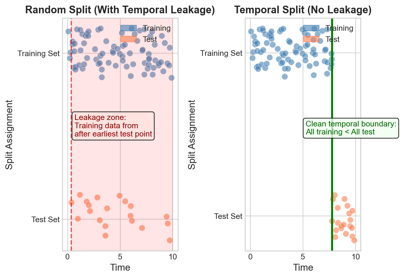
Figure 17.1: Temporal leakage in random splits versus proper temporal splits. Random splits intermingle observations from all time periods, allowing models to learn from future data when predicting past outcomes.
17.3 Taxonomy of Temporal Evaluation Strategies
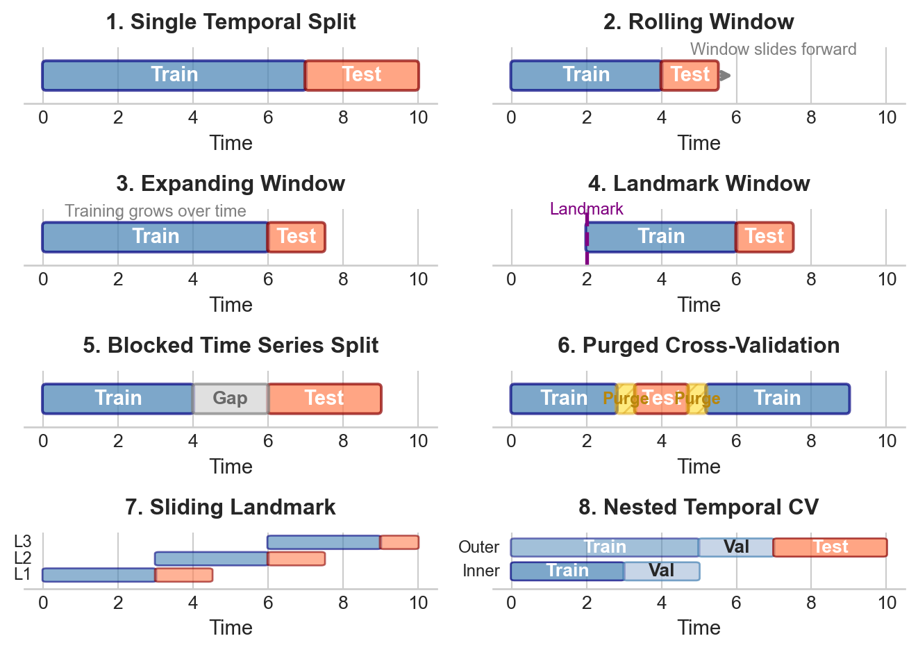
We present seven distinct temporal evaluation strategies, each addressing different assumptions about data structure, computational constraints, and evaluation goals.
Figure 17.2: Visual taxonomy of temporal evaluation strategies. Blue regions indicate training data; orange regions indicate test data; gray regions indicate gaps or embargo periods; hatched regions indicate purged observations.
17.4 Core Implementation Framework
We implement a unified framework for temporal cross-validation that supports all strategies through a common interface.
Base classes for temporal cross-validation
@dataclassclass TemporalFold:"""Container for a single temporal fold.""" fold_id: int train_indices: np.ndarray test_indices: np.ndarray train_start_time: float train_end_time: float test_start_time: float test_end_time: float gap_indices: Optional[np.ndarray] =None purge_indices: Optional[np.ndarray] =None@propertydef n_train(self) ->int:returnlen(self.train_indices)@propertydef n_test(self) ->int:returnlen(self.test_indices)class BaseTemporalCV:"""Base class for temporal cross-validation strategies."""def__init__(self):self.folds_ = []def split(self, X: np.ndarray, y: np.ndarray, timestamps: np.ndarray) -> Generator[TemporalFold, None, None]:"""Generate temporal folds. Override in subclasses."""raiseNotImplementedErrordef get_n_splits(self) ->int:"""Return number of folds."""returnlen(self.folds_)def evaluate(self, X: np.ndarray, y: np.ndarray, timestamps: np.ndarray, model_fn: Callable, metric_fn: Callable, return_predictions: bool=False) -> pd.DataFrame:""" Evaluate a model across all temporal folds. Parameters ---------- X : np.ndarray Features y : np.ndarray Target timestamps : np.ndarray Observation timestamps model_fn : Callable Function that returns a fresh model instance metric_fn : Callable Function(y_true, y_pred) -> score return_predictions : bool Whether to return predictions for each fold Returns ------- pd.DataFrame Results for each fold """ results = []for fold inself.split(X, y, timestamps): X_train = X[fold.train_indices] y_train = y[fold.train_indices] X_test = X[fold.test_indices] y_test = y[fold.test_indices]# Fit model model = model_fn() model.fit(X_train, y_train)# Predictifhasattr(model, 'predict_proba'): y_pred = model.predict_proba(X_test)[:, 1]else: y_pred = model.predict(X_test)# Compute metric score = metric_fn(y_test, y_pred) result = {'fold': fold.fold_id,'n_train': fold.n_train,'n_test': fold.n_test,'train_period': f"{fold.train_start_time:.2f}-{fold.train_end_time:.2f}",'test_period': f"{fold.test_start_time:.2f}-{fold.test_end_time:.2f}",'score': score }if return_predictions: result['y_test'] = y_test result['y_pred'] = y_pred results.append(result)return pd.DataFrame(results)
17.5 Method 1: Single Temporal Split
The simplest approach: sort by time, use earlier observations for training, later for testing (Tashman 2000).
Single temporal split implementation
class SingleTemporalSplit(BaseTemporalCV):""" Single temporal train/test split. The simplest temporal evaluation: all training observations occur before all test observations. Parameters ---------- train_fraction : float Fraction of data (by time order) for training """def__init__(self, train_fraction: float=0.8):super().__init__()ifnot0< train_fraction <1:raiseValueError("train_fraction must be between 0 and 1")self.train_fraction = train_fractiondef split(self, X: np.ndarray, y: np.ndarray, timestamps: np.ndarray) -> Generator[TemporalFold, None, None]: sorted_idx = np.argsort(timestamps) sorted_times = timestamps[sorted_idx] n =len(X) split_point =int(n *self.train_fraction)yield TemporalFold( fold_id=0, train_indices=sorted_idx[:split_point], test_indices=sorted_idx[split_point:], train_start_time=sorted_times[0], train_end_time=sorted_times[split_point -1], test_start_time=sorted_times[split_point], test_end_time=sorted_times[-1] )# Demonstrationprint("METHOD 1: SINGLE TEMPORAL SPLIT")print("="*70)cv = SingleTemporalSplit(train_fraction=0.8)results = cv.evaluate( X_clf, y_clf, t_clf, model_fn=lambda: LogisticRegression(max_iter=1000), metric_fn=roc_auc_score)print(results.to_string(index=False))
A fixed-size window slides forward, providing multiple evaluation points and revealing performance variation across time periods (Cerqueira, Torgo, and Mozetič 2020).
Rolling window cross-validation
class RollingWindowCV(BaseTemporalCV):""" Rolling window temporal cross-validation. A fixed-size training window slides forward through time. Useful when only recent history is relevant (e.g., non-stationary processes) or when you want to assess performance stability across time. Parameters ---------- n_splits : int Number of rolling windows train_fraction : float Fraction of total data in each training window test_fraction : float Fraction of total data in each test window """def__init__(self, n_splits: int=5, train_fraction: float=0.2, test_fraction: float=0.1):super().__init__()self.n_splits = n_splitsself.train_fraction = train_fractionself.test_fraction = test_fractiondef split(self, X: np.ndarray, y: np.ndarray, timestamps: np.ndarray) -> Generator[TemporalFold, None, None]: sorted_idx = np.argsort(timestamps) sorted_times = timestamps[sorted_idx] n =len(X) train_size =int(n *self.train_fraction) test_size =int(n *self.test_fraction)# Calculate step size to fit n_splits windows available = n - train_size - test_size step =max(1, available // (self.n_splits -1)) ifself.n_splits >1else0for i inrange(self.n_splits): train_start = i * step train_end = train_start + train_size test_start = train_end test_end =min(test_start + test_size, n)if test_end <= test_start:breakyield TemporalFold( fold_id=i, train_indices=sorted_idx[train_start:train_end], test_indices=sorted_idx[test_start:test_end], train_start_time=sorted_times[train_start], train_end_time=sorted_times[train_end -1], test_start_time=sorted_times[test_start], test_end_time=sorted_times[test_end -1] )print("\nMETHOD 2: ROLLING WINDOW")print("="*70)cv = RollingWindowCV(n_splits=5, train_fraction=0.3, test_fraction=0.1)results_rolling = cv.evaluate( X_clf, y_clf, t_clf, model_fn=lambda: LogisticRegression(max_iter=1000), metric_fn=roc_auc_score)print(results_rolling.to_string(index=False))print(f"\nMean AUC: {results_rolling['score'].mean():.4f} +/- {results_rolling['score'].std():.4f}")
Training data accumulates over time while test windows slide forward. Uses all available history, appropriate when older data remains relevant.
Expanding window cross-validation
class ExpandingWindowCV(BaseTemporalCV):""" Expanding window temporal cross-validation. Training data grows over time (uses all history up to each point), while test windows slide forward. Mimics deployment where you want to leverage all available historical data. Parameters ---------- n_splits : int Number of evaluation points initial_train_fraction : float Fraction of data for initial training set test_fraction : float Fraction of data in each test window """def__init__(self, n_splits: int=5, initial_train_fraction: float=0.4, test_fraction: float=0.1):super().__init__()self.n_splits = n_splitsself.initial_train_fraction = initial_train_fractionself.test_fraction = test_fractiondef split(self, X: np.ndarray, y: np.ndarray, timestamps: np.ndarray) -> Generator[TemporalFold, None, None]: sorted_idx = np.argsort(timestamps) sorted_times = timestamps[sorted_idx] n =len(X) initial_train =int(n *self.initial_train_fraction) test_size =int(n *self.test_fraction) available = n - initial_train - test_size step =max(1, available //self.n_splits) ifself.n_splits >0else availablefor i inrange(self.n_splits): train_end = initial_train + i * step test_start = train_end test_end =min(test_start + test_size, n)if test_end <= test_start or train_end >= n:breakyield TemporalFold( fold_id=i, train_indices=sorted_idx[:train_end], # Expanding: always from start test_indices=sorted_idx[test_start:test_end], train_start_time=sorted_times[0], train_end_time=sorted_times[train_end -1], test_start_time=sorted_times[test_start], test_end_time=sorted_times[test_end -1] )print("\nMETHOD 3: EXPANDING WINDOW")print("="*70)cv = ExpandingWindowCV(n_splits=5, initial_train_fraction=0.4, test_fraction=0.1)results_expanding = cv.evaluate( X_clf, y_clf, t_clf, model_fn=lambda: LogisticRegression(max_iter=1000), metric_fn=roc_auc_score)print(results_expanding.to_string(index=False))print(f"\nMean AUC: {results_expanding['score'].mean():.4f} +/- {results_expanding['score'].std():.4f}")
Inserts a gap between training and test periods to prevent leakage from temporal autocorrelation. Essential when recent observations are correlated with near-future outcomes in ways that don’t generalize.
Blocked time series split with embargo
class BlockedTimeSeriesCV(BaseTemporalCV):""" Blocked time series split with embargo period. Inserts a gap between training and test to prevent leakage from short-term temporal autocorrelation. Critical for financial and other high-frequency applications. Parameters ---------- n_splits : int Number of evaluation points train_fraction : float Fraction of data for training gap_fraction : float Fraction of data for embargo gap test_fraction : float Fraction of data for testing """def__init__(self, n_splits: int=5, train_fraction: float=0.5, gap_fraction: float=0.05, test_fraction: float=0.1):super().__init__()self.n_splits = n_splitsself.train_fraction = train_fractionself.gap_fraction = gap_fractionself.test_fraction = test_fractiondef split(self, X: np.ndarray, y: np.ndarray, timestamps: np.ndarray) -> Generator[TemporalFold, None, None]: sorted_idx = np.argsort(timestamps) sorted_times = timestamps[sorted_idx] n =len(X) train_size =int(n *self.train_fraction) gap_size =int(n *self.gap_fraction) test_size =int(n *self.test_fraction) window_size = train_size + gap_size + test_size available = n - window_size step =max(1, available // (self.n_splits -1)) ifself.n_splits >1else0for i inrange(self.n_splits): train_start = i * step train_end = train_start + train_size gap_start = train_end gap_end = gap_start + gap_size test_start = gap_end test_end =min(test_start + test_size, n)if test_end <= test_start:breakyield TemporalFold( fold_id=i, train_indices=sorted_idx[train_start:train_end], test_indices=sorted_idx[test_start:test_end], train_start_time=sorted_times[train_start], train_end_time=sorted_times[train_end -1], test_start_time=sorted_times[test_start], test_end_time=sorted_times[test_end -1], gap_indices=sorted_idx[gap_start:gap_end] )print("\nMETHOD 4: BLOCKED TIME SERIES SPLIT")print("="*70)cv = BlockedTimeSeriesCV(n_splits=5, train_fraction=0.4, gap_fraction=0.05, test_fraction=0.1)results_blocked = cv.evaluate( X_clf, y_clf, t_clf, model_fn=lambda: LogisticRegression(max_iter=1000), metric_fn=roc_auc_score)print(results_blocked.to_string(index=False))print(f"\nMean AUC: {results_blocked['score'].mean():.4f} +/- {results_blocked['score'].std():.4f}")
Generates multiple train/test combinations with purging, maximizing the number of evaluation points while respecting temporal structure.
Combinatorial purged cross-validation
class CombinatorialPurgedCV(BaseTemporalCV):""" Combinatorial Purged Cross-Validation. Generates multiple train/test combinations from k groups, with purging around test boundaries. Provides more evaluation points than standard k-fold while respecting temporal structure. Parameters ---------- n_groups : int Number of temporal groups to divide data into n_test_groups : int Number of groups to use as test in each fold purge_fraction : float Fraction of data to purge around test boundaries """def__init__(self, n_groups: int=6, n_test_groups: int=2, purge_fraction: float=0.01):super().__init__()self.n_groups = n_groupsself.n_test_groups = n_test_groupsself.purge_fraction = purge_fractiondef split(self, X: np.ndarray, y: np.ndarray, timestamps: np.ndarray) -> Generator[TemporalFold, None, None]:from itertools import combinations sorted_idx = np.argsort(timestamps) sorted_times = timestamps[sorted_idx] n =len(X)# Divide into groups group_size = n //self.n_groups purge_size =int(n *self.purge_fraction) groups = []for i inrange(self.n_groups): start = i * group_size end = (i +1) * group_size if i <self.n_groups -1else n groups.append((start, end))# Generate all combinations of test groups fold_id =0for test_group_indices in combinations(range(self.n_groups), self.n_test_groups):# Identify test indices test_mask = np.zeros(n, dtype=bool)for gi in test_group_indices: start, end = groups[gi] test_mask[start:end] =True# Identify purge regions (around test boundaries) purge_mask = np.zeros(n, dtype=bool)for gi in test_group_indices: start, end = groups[gi] purge_start =max(0, start - purge_size) purge_end =min(n, end + purge_size) purge_mask[purge_start:purge_end] =True# Training: everything not in test or purge train_mask =~purge_mask train_indices = sorted_idx[train_mask] test_indices = sorted_idx[test_mask]iflen(train_indices) ==0orlen(test_indices) ==0:continueyield TemporalFold( fold_id=fold_id, train_indices=train_indices, test_indices=test_indices, train_start_time=sorted_times[train_mask][0], train_end_time=sorted_times[train_mask][-1], test_start_time=sorted_times[test_mask][0], test_end_time=sorted_times[test_mask][-1], purge_indices=sorted_idx[purge_mask &~test_mask] ) fold_id +=1print("\nMETHOD 6: COMBINATORIAL PURGED CV")print("="*70)cv = CombinatorialPurgedCV(n_groups=5, n_test_groups=1, purge_fraction=0.02)results_combo = cv.evaluate( X_clf, y_clf, t_clf, model_fn=lambda: LogisticRegression(max_iter=1000), metric_fn=roc_auc_score)print(results_combo.to_string(index=False))print(f"\nMean AUC: {results_combo['score'].mean():.4f} +/- {results_combo['score'].std():.4f}")
COMPREHENSIVE METHOD COMPARISON
======================================================================
mean std
method
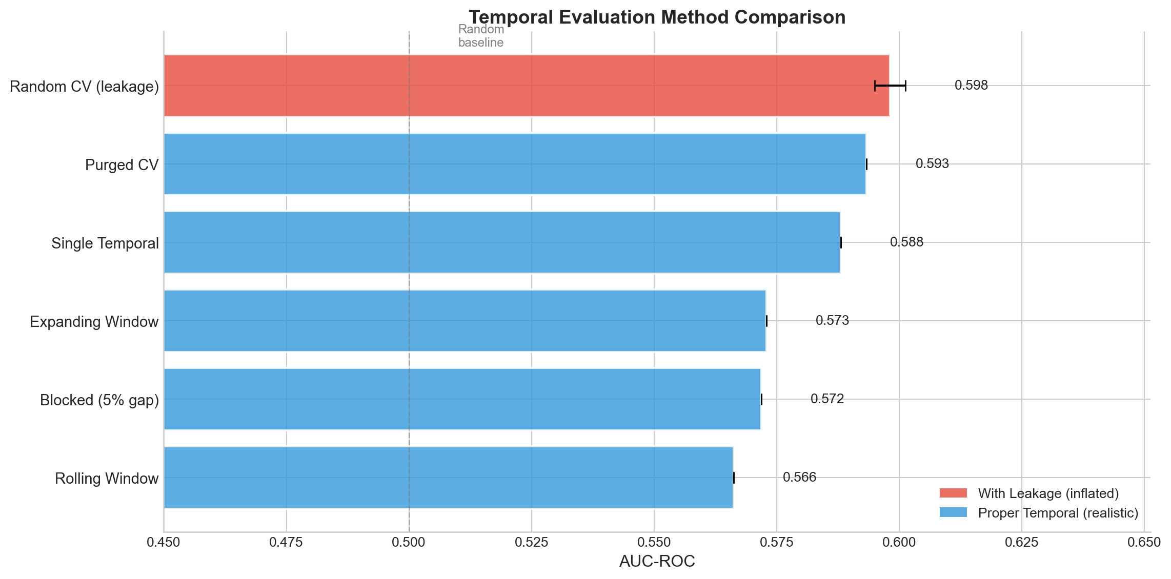
Random CV (leakage) 0.5981 0.0031
Purged CV 0.5933 0.0000
Single Temporal 0.5881 0.0000
Expanding Window 0.5729 0.0000
Blocked (5% gap) 0.5719 0.0000
Rolling Window 0.5662 0.0000
Code
fig, ax = plt.subplots(figsize=(12, 6))# Prepare datasummary_data = comparison_df.groupby('method')['score'].agg(['mean', 'std']).reset_index()summary_data = summary_data.sort_values('mean', ascending=True)# Color based on method typecolors = []for method in summary_data['method']:if'Random'in method or'leakage'in method: colors.append('#e74c3c') # Red for leaky methodelse: colors.append('#3498db') # Blue for proper temporal methodsbars = ax.barh(range(len(summary_data)), summary_data['mean'], xerr=summary_data['std'], capsize=4, color=colors, alpha=0.8, edgecolor='white', linewidth=1.5)ax.set_yticks(range(len(summary_data)))ax.set_yticklabels(summary_data['method'], fontsize=11)ax.set_xlabel('AUC-ROC', fontsize=12)ax.set_title('Temporal Evaluation Method Comparison', fontsize=14, fontweight='bold')# Reference lineax.axvline(x=0.5, color='gray', linestyle='--', alpha=0.5, linewidth=1)ax.text(0.51, len(summary_data) -0.5, 'Random\nbaseline', fontsize=9, color='gray')# Value labelsfor i, (mean, std) inenumerate(zip(summary_data['mean'], summary_data['std'])): ax.text(mean + std +0.01, i, f'{mean:.3f}', va='center', fontsize=10)# Legendfrom matplotlib.patches import Patchlegend_elements = [ Patch(facecolor='#e74c3c', alpha=0.8, label='With Leakage (inflated)'), Patch(facecolor='#3498db', alpha=0.8, label='Proper Temporal (realistic)')]ax.legend(handles=legend_elements, loc='lower right', fontsize=10)ax.set_xlim([0.45, summary_data['mean'].max() + summary_data['std'].max() +0.05])ax.spines['top'].set_visible(False)ax.spines['right'].set_visible(False)plt.tight_layout()plt.show()
Figure 17.3: Comparison of temporal evaluation methods. Random CV inflates performance estimates due to data leakage. Proper temporal methods provide more realistic (typically lower) estimates that better reflect deployment performance.
17.14 Decision Framework
flowchart TD
    A["Start Need Temporal Evaluation"] --> B{"Need hyperparameter tuning"}

    B -->|Yes| C["Use Nested Temporal CV"]
    B -->|No| D{"Strong temporal autocorrelation"}

    D -->|Yes| E{"Financial or high frequency data"}
    D -->|No| F{"Need variance estimates"}

    E -->|Yes| G["Use Purged CV or Combinatorial Purged CV"]
    E -->|No| H["Use Blocked Split with embargo gap"]

    F -->|Yes| I{"Older data still relevant"}
    F -->|No| J["Use Single Temporal Split"]

    I -->|Yes| K["Use Expanding Window"]
    I -->|No| L["Use Rolling Window"]

    C --> M[End]
    G --> M
    H --> M
    J --> M
    K --> M
    L --> M
Figure 17.4: Decision flowchart for selecting appropriate temporal evaluation strategy.
17.15 Summary: Method Selection Guide
Method
Best Use Case
Leakage Prevention
Variance Estimate
Computational Cost
Single Temporal
Quick baseline evaluation
Good
None
Very Low
Rolling Window
Non-stationary processes, recent data most relevant
Good
Good
Medium
Expanding Window
Stationary processes, all history valuable
Good
Good
Medium
Blocked Split
Autocorrelated data, need embargo
Very Good
Limited
Low
Purged CV
Financial applications, overlapping labels
Excellent
Good
High
Combinatorial Purged
Maximum rigor, many evaluation points
Excellent
Excellent
Very High
Nested Temporal
Hyperparameter tuning without bias
Excellent
Good
Very High
17.16 Using Existing Libraries
Several established libraries provide temporal cross-validation:
Report variance estimates, not just point estimates
17.17.2 Common Mistakes
Shuffling data before splitting (destroys temporal order)
Computing features using future information
Using sequential IDs that encode temporal information
Reusing the same test set during development
Ignoring concept drift in long time series
17.17.3 Reporting Standards
When publishing results with temporal evaluation:
Specify the exact temporal split strategy used
Report performance across multiple time windows
Include confidence intervals or standard errors
Compare against random CV baseline to quantify leakage
Describe any embargo or purging procedures
Cerqueira, Vitor, Luis Torgo, and Igor Mozetič. 2020. “Evaluating Time Series Forecasting Models: An Empirical Study on Performance Estimation Methods.”Machine Learning 109 (11): 1997–2028.
Kaufman, Shachar, Saharon Rosset, Claudia Perlich, and Ori Stitelman. 2012. “Leakage in Data Mining: Formulation, Detection, and Avoidance.”ACM Transactions on Knowledge Discovery from Data (TKDD) 6 (4): 1–21.
Tashman, Leonard J. 2000. “Out-of-Sample Tests of Forecasting Accuracy: An Analysis and Review.”International Journal of Forecasting 16 (4): 437–50.
Source Code
# Temporal Evaluation Strategies {#sec-temporal-evaluation}## Introduction: The Temporal Structure of Prediction ProblemsMost real-world prediction problems have an inherent temporal structure: we observe data up to time $t$ and wish to predict outcomes at time $t + h$. This structure creates a fundamental constraint that standard cross-validation ignores. When we randomly shuffle data into train and test sets, we allow the model to learn from "future" observations when predicting "past" ones.This chapter provides a systematic treatment of temporal evaluation strategies. While the examples focus on tabular prediction and time series, the principles apply broadly: recommendation systems, fraud detection, demand forecasting, clinical prediction, financial modeling, and any domain where data arrives sequentially and predictions concern future states.The consequences of ignoring temporal structure are well-documented. @kaufman2012leakage found that random cross-validation overestimated AUC in prediction models compared to temporal validation. Temporal evaluation is not a methodological nicety; it determines whether reported performance reflects deployment reality.```{python}#| label: setup#| code-summary: "Import required libraries"import numpy as npimport pandas as pdimport matplotlib.pyplot as pltimport matplotlib.patches as mpatchesfrom matplotlib.patches import FancyBboxPatch, FancyArrowPatchimport seaborn as snsfrom typing import List, Dict, Tuple, Callable, Optional, Generator, Unionfrom dataclasses import dataclass, fieldfrom sklearn.metrics import roc_auc_score, mean_squared_error, mean_absolute_errorfrom sklearn.linear_model import LogisticRegression, Ridgefrom sklearn.ensemble import RandomForestClassifier, GradientBoostingRegressorfrom sklearn.preprocessing import StandardScalerfrom scipy import statsimport warningswarnings.filterwarnings('ignore')plt.style.use('seaborn-v0_8-whitegrid')```## The Data Leakage Problem### Formalizing Temporal LeakageConsider a supervised learning problem with observations $\{(x_i, y_i, t_i)\}_{i=1}^{n}$ where $x_i$ are features, $y_i$ is the target, and $t_i$ is the observation timestamp. The prediction task at time $t$ requires estimating $y$ for observations arriving after $t$, using only information available before $t$.**Definition (Temporal Leakage):** A training procedure exhibits temporal leakage if model parameters $\theta$ depend on observations $(x_i, y_i)$ where $t_i \geq t_{eval}$, the evaluation time.Random $k$-fold cross-validation creates leakage because each fold's training set includes observations from all time periods. The expected fraction of training observations temporally after any given test observation is approximately $(k-1)/(2k)$.### Quantifying Leakage Impact```{python}#| label: generate-temporal-data#| code-summary: "Generate synthetic temporal dataset with concept drift"def generate_temporal_classification_data( n_samples: int=5000, n_features: int=20, n_periods: int=10, drift_strength: float=0.3, noise_level: float=0.2) -> Tuple[np.ndarray, np.ndarray, np.ndarray]:""" Generate temporal classification data with concept drift. The decision boundary shifts over time, making future information particularly valuable and leakage particularly harmful. Parameters ---------- n_samples : int Total number of observations n_features : int Number of features n_periods : int Number of discrete time periods drift_strength : float How much the true coefficients change over time noise_level : float Label noise probability Returns ------- X : np.ndarray Features of shape (n_samples, n_features) y : np.ndarray Binary labels timestamps : np.ndarray Observation timestamps """ np.random.seed(42) samples_per_period = n_samples // n_periods# Initial true coefficients true_coef = np.random.randn(n_features) true_coef = true_coef / np.linalg.norm(true_coef) X_list, y_list, t_list = [], [], []for period inrange(n_periods):# Drift coefficients over time drift = np.random.randn(n_features) * drift_strength * (period / n_periods) current_coef = true_coef + drift current_coef = current_coef / np.linalg.norm(current_coef)# Generate features X_period = np.random.randn(samples_per_period, n_features)# Generate labels based on current decision boundary logits = X_period @ current_coef probs =1/ (1+ np.exp(-logits)) y_period = (np.random.random(samples_per_period) < probs).astype(int)# Add label noise flip_mask = np.random.random(samples_per_period) < noise_level y_period[flip_mask] =1- y_period[flip_mask]# Timestamps within period t_period = period + np.random.uniform(0, 1, samples_per_period) X_list.append(X_period) y_list.append(y_period) t_list.append(t_period)return np.vstack(X_list), np.concatenate(y_list), np.concatenate(t_list)def generate_temporal_regression_data( n_samples: int=5000, n_features: int=20, n_periods: int=10, drift_strength: float=0.5, noise_std: float=0.5) -> Tuple[np.ndarray, np.ndarray, np.ndarray]:"""Generate temporal regression data with concept drift.""" np.random.seed(42) samples_per_period = n_samples // n_periods true_coef = np.random.randn(n_features) X_list, y_list, t_list = [], [], []for period inrange(n_periods): drift = np.random.randn(n_features) * drift_strength * (period / n_periods) current_coef = true_coef + drift X_period = np.random.randn(samples_per_period, n_features) y_period = X_period @ current_coef + np.random.randn(samples_per_period) * noise_std t_period = period + np.random.uniform(0, 1, samples_per_period) X_list.append(X_period) y_list.append(y_period) t_list.append(t_period)return np.vstack(X_list), np.concatenate(y_list), np.concatenate(t_list)# Generate datasetsX_clf, y_clf, t_clf = generate_temporal_classification_data( n_samples=5000, drift_strength=0.5)X_reg, y_reg, t_reg = generate_temporal_regression_data( n_samples=5000, drift_strength=0.5)print("Generated temporal datasets:")print(f" Classification: {X_clf.shape[0]} samples, {X_clf.shape[1]} features")print(f" Regression: {X_reg.shape[0]} samples, {X_reg.shape[1]} features")print(f" Time span: {t_clf.min():.1f} to {t_clf.max():.1f}")``````{python}#| label: leakage-demonstration#| code-summary: "Demonstrate performance inflation from temporal leakage"from sklearn.model_selection import cross_val_score, KFolddef evaluate_with_leakage(X, y, timestamps, model, n_trials=10):"""Compare random CV (with leakage) vs temporal split (no leakage).""" random_scores = [] temporal_scores = []for trial inrange(n_trials):# Random CV (introduces leakage) cv = KFold(n_splits=5, shuffle=True, random_state=trial) scores = cross_val_score(model, X, y, cv=cv, scoring='roc_auc') random_scores.append(scores.mean())# Temporal split (no leakage) sorted_idx = np.argsort(timestamps) split_point =int(0.8*len(X)) train_idx = sorted_idx[:split_point] test_idx = sorted_idx[split_point:] X_train, X_test = X[train_idx], X[test_idx] y_train, y_test = y[train_idx], y[test_idx] model_clone = LogisticRegression(max_iter=1000, random_state=trial) model_clone.fit(X_train, y_train)iflen(np.unique(y_test)) >1: score = roc_auc_score(y_test, model_clone.predict_proba(X_test)[:, 1]) temporal_scores.append(score)return {'random_cv_mean': np.mean(random_scores),'random_cv_std': np.std(random_scores),'temporal_mean': np.mean(temporal_scores),'temporal_std': np.std(temporal_scores),'inflation': np.mean(random_scores) - np.mean(temporal_scores) }print("TEMPORAL LEAKAGE IMPACT")print("="*70)model = LogisticRegression(max_iter=1000)results = evaluate_with_leakage(X_clf, y_clf, t_clf, model)print(f"\nRandom 5-Fold CV (with leakage):")print(f" AUC = {results['random_cv_mean']:.4f} +/- {results['random_cv_std']:.4f}")print(f"\nTemporal Split (no leakage):")print(f" AUC = {results['temporal_mean']:.4f} +/- {results['temporal_std']:.4f}")print(f"\nPerformance Inflation: {results['inflation']:.4f} ({results['inflation']*100:.1f} percentage points)")```### Visualizing Temporal Leakage```{python}#| label: fig-leakage-visualization#| fig-cap: "Temporal leakage in random splits versus proper temporal splits. Random splits intermingle observations from all time periods, allowing models to learn from future data when predicting past outcomes."#| fig-width: 7fig, axes = plt.subplots(1, 2)np.random.seed(42)n_points =100times = np.sort(np.random.uniform(0, 10, n_points))# Random split assignmentperm = np.random.permutation(n_points)random_train_mask = np.zeros(n_points, dtype=bool)random_train_mask[perm[:80]] =True# Temporal splittemporal_split_time = times[80]temporal_train_mask = times < temporal_split_time# Panel 1: Random Splitax1 = axes[0]jitter = np.random.uniform(-0.15, 0.15, n_points)ax1.scatter(times[random_train_mask], np.ones(sum(random_train_mask)) + jitter[random_train_mask], c='steelblue', s=60, alpha=0.6, edgecolors='white', linewidth=0.5)ax1.scatter(times[~random_train_mask], np.zeros(sum(~random_train_mask)) + jitter[~random_train_mask], c='coral', s=60, alpha=0.6, edgecolors='white', linewidth=0.5)# Highlight leakage regionmin_test_time = times[~random_train_mask].min()ax1.axvspan(min_test_time, 10, alpha=0.1, color='red')ax1.axvline(x=min_test_time, color='red', linestyle='--', alpha=0.7, linewidth=1.5)ax1.annotate('Leakage zone:\nTraining data from\nafter earliest test point', xy=(min_test_time +0.3, 0.5), fontsize=10, color='darkred', bbox=dict(boxstyle='round', facecolor='mistyrose', alpha=0.8))ax1.set_xlabel('Time', fontsize=12)ax1.set_ylabel('Split Assignment', fontsize=12)ax1.set_yticks([0, 1])ax1.set_yticklabels(['Test Set', 'Training Set'])ax1.set_title('Random Split (With Temporal Leakage)', fontsize=13, fontweight='bold')ax1.set_xlim(-0.5, 10.5)# Panel 2: Temporal Splitax2 = axes[1]ax2.scatter(times[temporal_train_mask], np.ones(sum(temporal_train_mask)) + jitter[temporal_train_mask], c='steelblue', s=60, alpha=0.6, edgecolors='white', linewidth=0.5)ax2.scatter(times[~temporal_train_mask], np.zeros(sum(~temporal_train_mask)) + jitter[~temporal_train_mask], c='coral', s=60, alpha=0.6, edgecolors='white', linewidth=0.5)ax2.axvline(x=temporal_split_time, color='green', linestyle='-', linewidth=2.5)ax2.annotate('Clean temporal boundary:\nAll training < All test', xy=(temporal_split_time -2.5, 0.5), fontsize=10, color='darkgreen', bbox=dict(boxstyle='round', facecolor='honeydew', alpha=0.8))ax2.set_xlabel('Time', fontsize=12)ax2.set_ylabel('Split Assignment', fontsize=12)ax2.set_yticks([0, 1])ax2.set_yticklabels(['Test Set', 'Training Set'])ax2.set_title('Temporal Split (No Leakage)', fontsize=13, fontweight='bold')ax2.set_xlim(-0.5, 10.5)# Add legendsfor ax in axes: train_patch = mpatches.Patch(color='steelblue', alpha=0.6, label='Training') test_patch = mpatches.Patch(color='coral', alpha=0.6, label='Test') ax.legend(handles=[train_patch, test_patch], loc='upper right')plt.tight_layout()plt.show()```## Taxonomy of Temporal Evaluation StrategiesWe present seven distinct temporal evaluation strategies, each addressing different assumptions about data structure, computational constraints, and evaluation goals.```{python}#| label: fig-temporal-methods-taxonomy#| fig-cap: "Visual taxonomy of temporal evaluation strategies. Blue regions indicate training data; orange regions indicate test data; gray regions indicate gaps or embargo periods; hatched regions indicate purged observations."fig, axes = plt.subplots(4, 2)def draw_split_diagram(ax, train_regions, test_regions, title, gap_regions=None, purge_regions=None, annotations=None):"""Draw a temporal split diagram.""" ax.set_xlim(-0.5, 10.5) ax.set_ylim(-0.3, 1.3)# Draw train regionsfor start, end in train_regions: rect = FancyBboxPatch((start, 0.1), end - start, 0.8, boxstyle="round,pad=0.02,rounding_size=0.1", facecolor='steelblue', alpha=0.7, edgecolor='navy', linewidth=1.5) ax.add_patch(rect) ax.text((start + end) /2, 0.5, 'Train', ha='center', va='center', fontsize=11, color='white', fontweight='bold')# Draw test regionsfor start, end in test_regions: rect = FancyBboxPatch((start, 0.1), end - start, 0.8, boxstyle="round,pad=0.02,rounding_size=0.1", facecolor='coral', alpha=0.7, edgecolor='darkred', linewidth=1.5) ax.add_patch(rect) ax.text((start + end) /2, 0.5, 'Test', ha='center', va='center', fontsize=11, color='white', fontweight='bold')# Draw gap regionsif gap_regions:for start, end in gap_regions: rect = FancyBboxPatch((start, 0.1), end - start, 0.8, boxstyle="round,pad=0.02,rounding_size=0.1", facecolor='lightgray', alpha=0.7, edgecolor='gray', linewidth=1.5) ax.add_patch(rect) ax.text((start + end) /2, 0.5, 'Gap', ha='center', va='center', fontsize=10, color='dimgray', fontweight='bold')# Draw purge regionsif purge_regions:for start, end in purge_regions: rect = FancyBboxPatch((start, 0.1), end - start, 0.8, boxstyle="round,pad=0.02,rounding_size=0.1", facecolor='gold', alpha=0.5, edgecolor='goldenrod', linewidth=1.5, hatch='///') ax.add_patch(rect) ax.text((start + end) /2, 0.5, 'Purge', ha='center', va='center', fontsize=9, color='darkgoldenrod', fontweight='bold')# Add annotationsif annotations:for ann in annotations: ax.annotate(ann['text'], xy=ann['xy'], fontsize=9, ha='center', color=ann.get('color', 'black')) ax.set_xlabel('Time', fontsize=11) ax.set_yticks([]) ax.set_title(title, fontsize=12, fontweight='bold', pad=10) ax.set_xticks(range(0, 11, 2)) ax.spines['top'].set_visible(False) ax.spines['right'].set_visible(False) ax.spines['left'].set_visible(False)# 1. Single Temporal Splitdraw_split_diagram(axes[0, 0], [(0, 7)], [(7, 10)], "1. Single Temporal Split")# 2. Rolling Windowdraw_split_diagram(axes[0, 1], [(0, 4)], [(4, 5.5)],"2. Rolling Window", annotations=[{'text': 'Window slides forward', 'xy': (7, 1.1), 'color': 'gray'}])# Add arrow for slidingaxes[0, 1].annotate('', xy=(6, 0.5), xytext=(5.5, 0.5), arrowprops=dict(arrowstyle='->', color='gray', lw=2))# 3. Expanding Windowdraw_split_diagram(axes[1, 0], [(0, 6)], [(6, 7.5)],"3. Expanding Window", annotations=[{'text': 'Training grows over time', 'xy': (3, 1.1), 'color': 'gray'}])# 4. Landmark Windowdraw_split_diagram(axes[1, 1], [(2, 6)], [(6, 7.5)],"4. Landmark Window", annotations=[{'text': 'Landmark', 'xy': (2, 1.15), 'color': 'purple'}])axes[1, 1].axvline(x=2, color='purple', linestyle='--', linewidth=2)# 5. Blocked Time Series (with gap)draw_split_diagram(axes[2, 0], [(0, 4)], [(6, 9)],"5. Blocked Time Series Split", gap_regions=[(4, 6)])# 6. Purged Cross-Validationdraw_split_diagram(axes[2, 1], [(0, 2.8), (5.2, 9)], [(3.3, 4.7)],"6. Purged Cross-Validation", purge_regions=[(2.8, 3.3), (4.7, 5.2)])# 7. Sliding Landmark (multiple)ax = axes[3, 0]ax.set_xlim(-0.5, 10.5)ax.set_ylim(-0.3, 2.8)for i, (train_start, train_end, test_start, test_end) inenumerate([ (0, 3, 3, 4.5), (3, 6, 6, 7.5), (6, 9, 9, 10)]): y_offset = i *0.9 rect_train = FancyBboxPatch((train_start, 0.1+ y_offset), train_end - train_start, 0.7, boxstyle="round,pad=0.02,rounding_size=0.1", facecolor='steelblue', alpha=0.6, edgecolor='navy', linewidth=1) ax.add_patch(rect_train) rect_test = FancyBboxPatch((test_start, 0.1+ y_offset), test_end - test_start, 0.7, boxstyle="round,pad=0.02,rounding_size=0.1", facecolor='coral', alpha=0.6, edgecolor='darkred', linewidth=1) ax.add_patch(rect_test) ax.text(-0.3, 0.45+ y_offset, f'L{i+1}', ha='right', va='center', fontsize=9)ax.set_xlabel('Time', fontsize=11)ax.set_yticks([])ax.set_title("7. Sliding Landmark", fontsize=12, fontweight='bold', pad=10)ax.set_xticks(range(0, 11, 2))ax.spines['top'].set_visible(False)ax.spines['right'].set_visible(False)ax.spines['left'].set_visible(False)# 8. Nested Temporal CVax = axes[3, 1]ax.set_xlim(-0.5, 10.5)ax.set_ylim(-0.3, 2.3)# Outer looprect = FancyBboxPatch((0, 1.2), 5, 0.8, boxstyle="round,pad=0.02,rounding_size=0.1", facecolor='steelblue', alpha=0.5, edgecolor='navy', linewidth=1)ax.add_patch(rect)rect = FancyBboxPatch((5, 1.2), 2, 0.8, boxstyle="round,pad=0.02,rounding_size=0.1", facecolor='lightsteelblue', alpha=0.7, edgecolor='steelblue', linewidth=1)ax.add_patch(rect)rect = FancyBboxPatch((7, 1.2), 3, 0.8, boxstyle="round,pad=0.02,rounding_size=0.1", facecolor='coral', alpha=0.7, edgecolor='darkred', linewidth=1)ax.add_patch(rect)ax.text(2.5, 1.6, 'Train', ha='center', va='center', fontsize=10, color='white', fontweight='bold')ax.text(6, 1.6, 'Val', ha='center', va='center', fontsize=10, fontweight='bold')ax.text(8.5, 1.6, 'Test', ha='center', va='center', fontsize=10, color='white', fontweight='bold')ax.text(-0.3, 1.6, 'Outer', ha='right', va='center', fontsize=9)# Inner looprect = FancyBboxPatch((0, 0.1), 3, 0.8, boxstyle="round,pad=0.02,rounding_size=0.1", facecolor='steelblue', alpha=0.7, edgecolor='navy', linewidth=1)ax.add_patch(rect)rect = FancyBboxPatch((3, 0.1), 2, 0.8, boxstyle="round,pad=0.02,rounding_size=0.1", facecolor='lightsteelblue', alpha=0.7, edgecolor='steelblue', linewidth=1)ax.add_patch(rect)ax.text(1.5, 0.5, 'Train', ha='center', va='center', fontsize=10, color='white', fontweight='bold')ax.text(4, 0.5, 'Val', ha='center', va='center', fontsize=10, fontweight='bold')ax.text(-0.3, 0.5, 'Inner', ha='right', va='center', fontsize=9)ax.set_xlabel('Time', fontsize=11)ax.set_yticks([])ax.set_title("8. Nested Temporal CV", fontsize=12, fontweight='bold', pad=10)ax.set_xticks(range(0, 11, 2))ax.spines['top'].set_visible(False)ax.spines['right'].set_visible(False)ax.spines['left'].set_visible(False)plt.tight_layout()plt.show()```## Core Implementation FrameworkWe implement a unified framework for temporal cross-validation that supports all strategies through a common interface.```{python}#| label: base-classes#| code-summary: "Base classes for temporal cross-validation"@dataclassclass TemporalFold:"""Container for a single temporal fold.""" fold_id: int train_indices: np.ndarray test_indices: np.ndarray train_start_time: float train_end_time: float test_start_time: float test_end_time: float gap_indices: Optional[np.ndarray] =None purge_indices: Optional[np.ndarray] =None@propertydef n_train(self) ->int:returnlen(self.train_indices)@propertydef n_test(self) ->int:returnlen(self.test_indices)class BaseTemporalCV:"""Base class for temporal cross-validation strategies."""def__init__(self):self.folds_ = []def split(self, X: np.ndarray, y: np.ndarray, timestamps: np.ndarray) -> Generator[TemporalFold, None, None]:"""Generate temporal folds. Override in subclasses."""raiseNotImplementedErrordef get_n_splits(self) ->int:"""Return number of folds."""returnlen(self.folds_)def evaluate(self, X: np.ndarray, y: np.ndarray, timestamps: np.ndarray, model_fn: Callable, metric_fn: Callable, return_predictions: bool=False) -> pd.DataFrame:""" Evaluate a model across all temporal folds. Parameters ---------- X : np.ndarray Features y : np.ndarray Target timestamps : np.ndarray Observation timestamps model_fn : Callable Function that returns a fresh model instance metric_fn : Callable Function(y_true, y_pred) -> score return_predictions : bool Whether to return predictions for each fold Returns ------- pd.DataFrame Results for each fold """ results = []for fold inself.split(X, y, timestamps): X_train = X[fold.train_indices] y_train = y[fold.train_indices] X_test = X[fold.test_indices] y_test = y[fold.test_indices]# Fit model model = model_fn() model.fit(X_train, y_train)# Predictifhasattr(model, 'predict_proba'): y_pred = model.predict_proba(X_test)[:, 1]else: y_pred = model.predict(X_test)# Compute metric score = metric_fn(y_test, y_pred) result = {'fold': fold.fold_id,'n_train': fold.n_train,'n_test': fold.n_test,'train_period': f"{fold.train_start_time:.2f}-{fold.train_end_time:.2f}",'test_period': f"{fold.test_start_time:.2f}-{fold.test_end_time:.2f}",'score': score }if return_predictions: result['y_test'] = y_test result['y_pred'] = y_pred results.append(result)return pd.DataFrame(results)```## Method 1: Single Temporal SplitThe simplest approach: sort by time, use earlier observations for training, later for testing [@tashman2000out].```{python}#| label: single-temporal-split#| code-summary: "Single temporal split implementation"class SingleTemporalSplit(BaseTemporalCV):""" Single temporal train/test split. The simplest temporal evaluation: all training observations occur before all test observations. Parameters ---------- train_fraction : float Fraction of data (by time order) for training """def__init__(self, train_fraction: float=0.8):super().__init__()ifnot0< train_fraction <1:raiseValueError("train_fraction must be between 0 and 1")self.train_fraction = train_fractiondef split(self, X: np.ndarray, y: np.ndarray, timestamps: np.ndarray) -> Generator[TemporalFold, None, None]: sorted_idx = np.argsort(timestamps) sorted_times = timestamps[sorted_idx] n =len(X) split_point =int(n *self.train_fraction)yield TemporalFold( fold_id=0, train_indices=sorted_idx[:split_point], test_indices=sorted_idx[split_point:], train_start_time=sorted_times[0], train_end_time=sorted_times[split_point -1], test_start_time=sorted_times[split_point], test_end_time=sorted_times[-1] )# Demonstrationprint("METHOD 1: SINGLE TEMPORAL SPLIT")print("="*70)cv = SingleTemporalSplit(train_fraction=0.8)results = cv.evaluate( X_clf, y_clf, t_clf, model_fn=lambda: LogisticRegression(max_iter=1000), metric_fn=roc_auc_score)print(results.to_string(index=False))```## Method 2: Rolling WindowA fixed-size window slides forward, providing multiple evaluation points and revealing performance variation across time periods [@cerqueira2020evaluating].```{python}#| label: rolling-window#| code-summary: "Rolling window cross-validation"class RollingWindowCV(BaseTemporalCV):""" Rolling window temporal cross-validation. A fixed-size training window slides forward through time. Useful when only recent history is relevant (e.g., non-stationary processes) or when you want to assess performance stability across time. Parameters ---------- n_splits : int Number of rolling windows train_fraction : float Fraction of total data in each training window test_fraction : float Fraction of total data in each test window """def__init__(self, n_splits: int=5, train_fraction: float=0.2, test_fraction: float=0.1):super().__init__()self.n_splits = n_splitsself.train_fraction = train_fractionself.test_fraction = test_fractiondef split(self, X: np.ndarray, y: np.ndarray, timestamps: np.ndarray) -> Generator[TemporalFold, None, None]: sorted_idx = np.argsort(timestamps) sorted_times = timestamps[sorted_idx] n =len(X) train_size =int(n *self.train_fraction) test_size =int(n *self.test_fraction)# Calculate step size to fit n_splits windows available = n - train_size - test_size step =max(1, available // (self.n_splits -1)) ifself.n_splits >1else0for i inrange(self.n_splits): train_start = i * step train_end = train_start + train_size test_start = train_end test_end =min(test_start + test_size, n)if test_end <= test_start:breakyield TemporalFold( fold_id=i, train_indices=sorted_idx[train_start:train_end], test_indices=sorted_idx[test_start:test_end], train_start_time=sorted_times[train_start], train_end_time=sorted_times[train_end -1], test_start_time=sorted_times[test_start], test_end_time=sorted_times[test_end -1] )print("\nMETHOD 2: ROLLING WINDOW")print("="*70)cv = RollingWindowCV(n_splits=5, train_fraction=0.3, test_fraction=0.1)results_rolling = cv.evaluate( X_clf, y_clf, t_clf, model_fn=lambda: LogisticRegression(max_iter=1000), metric_fn=roc_auc_score)print(results_rolling.to_string(index=False))print(f"\nMean AUC: {results_rolling['score'].mean():.4f} +/- {results_rolling['score'].std():.4f}")```## Method 3: Expanding WindowTraining data accumulates over time while test windows slide forward. Uses all available history, appropriate when older data remains relevant.```{python}#| label: expanding-window#| code-summary: "Expanding window cross-validation"class ExpandingWindowCV(BaseTemporalCV):""" Expanding window temporal cross-validation. Training data grows over time (uses all history up to each point), while test windows slide forward. Mimics deployment where you want to leverage all available historical data. Parameters ---------- n_splits : int Number of evaluation points initial_train_fraction : float Fraction of data for initial training set test_fraction : float Fraction of data in each test window """def__init__(self, n_splits: int=5, initial_train_fraction: float=0.4, test_fraction: float=0.1):super().__init__()self.n_splits = n_splitsself.initial_train_fraction = initial_train_fractionself.test_fraction = test_fractiondef split(self, X: np.ndarray, y: np.ndarray, timestamps: np.ndarray) -> Generator[TemporalFold, None, None]: sorted_idx = np.argsort(timestamps) sorted_times = timestamps[sorted_idx] n =len(X) initial_train =int(n *self.initial_train_fraction) test_size =int(n *self.test_fraction) available = n - initial_train - test_size step =max(1, available //self.n_splits) ifself.n_splits >0else availablefor i inrange(self.n_splits): train_end = initial_train + i * step test_start = train_end test_end =min(test_start + test_size, n)if test_end <= test_start or train_end >= n:breakyield TemporalFold( fold_id=i, train_indices=sorted_idx[:train_end], # Expanding: always from start test_indices=sorted_idx[test_start:test_end], train_start_time=sorted_times[0], train_end_time=sorted_times[train_end -1], test_start_time=sorted_times[test_start], test_end_time=sorted_times[test_end -1] )print("\nMETHOD 3: EXPANDING WINDOW")print("="*70)cv = ExpandingWindowCV(n_splits=5, initial_train_fraction=0.4, test_fraction=0.1)results_expanding = cv.evaluate( X_clf, y_clf, t_clf, model_fn=lambda: LogisticRegression(max_iter=1000), metric_fn=roc_auc_score)print(results_expanding.to_string(index=False))print(f"\nMean AUC: {results_expanding['score'].mean():.4f} +/- {results_expanding['score'].std():.4f}")```## Method 4: Blocked Time Series SplitInserts a gap between training and test periods to prevent leakage from temporal autocorrelation. Essential when recent observations are correlated with near-future outcomes in ways that don't generalize.```{python}#| label: blocked-split#| code-summary: "Blocked time series split with embargo"class BlockedTimeSeriesCV(BaseTemporalCV):""" Blocked time series split with embargo period. Inserts a gap between training and test to prevent leakage from short-term temporal autocorrelation. Critical for financial and other high-frequency applications. Parameters ---------- n_splits : int Number of evaluation points train_fraction : float Fraction of data for training gap_fraction : float Fraction of data for embargo gap test_fraction : float Fraction of data for testing """def__init__(self, n_splits: int=5, train_fraction: float=0.5, gap_fraction: float=0.05, test_fraction: float=0.1):super().__init__()self.n_splits = n_splitsself.train_fraction = train_fractionself.gap_fraction = gap_fractionself.test_fraction = test_fractiondef split(self, X: np.ndarray, y: np.ndarray, timestamps: np.ndarray) -> Generator[TemporalFold, None, None]: sorted_idx = np.argsort(timestamps) sorted_times = timestamps[sorted_idx] n =len(X) train_size =int(n *self.train_fraction) gap_size =int(n *self.gap_fraction) test_size =int(n *self.test_fraction) window_size = train_size + gap_size + test_size available = n - window_size step =max(1, available // (self.n_splits -1)) ifself.n_splits >1else0for i inrange(self.n_splits): train_start = i * step train_end = train_start + train_size gap_start = train_end gap_end = gap_start + gap_size test_start = gap_end test_end =min(test_start + test_size, n)if test_end <= test_start:breakyield TemporalFold( fold_id=i, train_indices=sorted_idx[train_start:train_end], test_indices=sorted_idx[test_start:test_end], train_start_time=sorted_times[train_start], train_end_time=sorted_times[train_end -1], test_start_time=sorted_times[test_start], test_end_time=sorted_times[test_end -1], gap_indices=sorted_idx[gap_start:gap_end] )print("\nMETHOD 4: BLOCKED TIME SERIES SPLIT")print("="*70)cv = BlockedTimeSeriesCV(n_splits=5, train_fraction=0.4, gap_fraction=0.05, test_fraction=0.1)results_blocked = cv.evaluate( X_clf, y_clf, t_clf, model_fn=lambda: LogisticRegression(max_iter=1000), metric_fn=roc_auc_score)print(results_blocked.to_string(index=False))print(f"\nMean AUC: {results_blocked['score'].mean():.4f} +/- {results_blocked['score'].std():.4f}")```## Method 5: Purged Cross-ValidationPurged cross-validation removes observations near the train/test boundary to prevent subtle leakage from overlapping information sets.```{python}#| label: purged-cv#| code-summary: "Purged k-fold cross-validation"class PurgedKFoldCV(BaseTemporalCV):""" Purged K-Fold cross-validation for temporal data. Removes training observations near the test set boundary to prevent leakage from overlapping information windows. Parameters ---------- n_splits : int Number of folds purge_fraction : float Fraction of data to purge around test boundaries """def__init__(self, n_splits: int=5, purge_fraction: float=0.01):super().__init__()self.n_splits = n_splitsself.purge_fraction = purge_fractiondef split(self, X: np.ndarray, y: np.ndarray, timestamps: np.ndarray) -> Generator[TemporalFold, None, None]: sorted_idx = np.argsort(timestamps) sorted_times = timestamps[sorted_idx] n =len(X) fold_size = n //self.n_splits purge_size =int(n *self.purge_fraction)for i inrange(self.n_splits): test_start = i * fold_size test_end = (i +1) * fold_size if i <self.n_splits -1else n# Purge regions around test set purge_before_start =max(0, test_start - purge_size) purge_after_end =min(n, test_end + purge_size)# Training: exclude test and purge regions train_mask = np.ones(n, dtype=bool) train_mask[purge_before_start:purge_after_end] =False train_indices = sorted_idx[train_mask] test_indices = sorted_idx[test_start:test_end] purge_indices = np.concatenate([ sorted_idx[purge_before_start:test_start], sorted_idx[test_end:purge_after_end] ])iflen(train_indices) ==0orlen(test_indices) ==0:continueyield TemporalFold( fold_id=i, train_indices=train_indices, test_indices=test_indices, train_start_time=sorted_times[train_mask][0] ifany(train_mask) else0, train_end_time=sorted_times[train_mask][-1] ifany(train_mask) else0, test_start_time=sorted_times[test_start], test_end_time=sorted_times[test_end -1], purge_indices=purge_indices )print("\nMETHOD 5: PURGED K-FOLD CV")print("="*70)cv = PurgedKFoldCV(n_splits=5, purge_fraction=0.02)results_purged = cv.evaluate( X_clf, y_clf, t_clf, model_fn=lambda: LogisticRegression(max_iter=1000), metric_fn=roc_auc_score)print(results_purged.to_string(index=False))print(f"\nMean AUC: {results_purged['score'].mean():.4f} +/- {results_purged['score'].std():.4f}")```## Method 6: Combinatorial Purged Cross-ValidationGenerates multiple train/test combinations with purging, maximizing the number of evaluation points while respecting temporal structure.```{python}#| label: combinatorial-purged-cv#| code-summary: "Combinatorial purged cross-validation"class CombinatorialPurgedCV(BaseTemporalCV):""" Combinatorial Purged Cross-Validation. Generates multiple train/test combinations from k groups, with purging around test boundaries. Provides more evaluation points than standard k-fold while respecting temporal structure. Parameters ---------- n_groups : int Number of temporal groups to divide data into n_test_groups : int Number of groups to use as test in each fold purge_fraction : float Fraction of data to purge around test boundaries """def__init__(self, n_groups: int=6, n_test_groups: int=2, purge_fraction: float=0.01):super().__init__()self.n_groups = n_groupsself.n_test_groups = n_test_groupsself.purge_fraction = purge_fractiondef split(self, X: np.ndarray, y: np.ndarray, timestamps: np.ndarray) -> Generator[TemporalFold, None, None]:from itertools import combinations sorted_idx = np.argsort(timestamps) sorted_times = timestamps[sorted_idx] n =len(X)# Divide into groups group_size = n //self.n_groups purge_size =int(n *self.purge_fraction) groups = []for i inrange(self.n_groups): start = i * group_size end = (i +1) * group_size if i <self.n_groups -1else n groups.append((start, end))# Generate all combinations of test groups fold_id =0for test_group_indices in combinations(range(self.n_groups), self.n_test_groups):# Identify test indices test_mask = np.zeros(n, dtype=bool)for gi in test_group_indices: start, end = groups[gi] test_mask[start:end] =True# Identify purge regions (around test boundaries) purge_mask = np.zeros(n, dtype=bool)for gi in test_group_indices: start, end = groups[gi] purge_start =max(0, start - purge_size) purge_end =min(n, end + purge_size) purge_mask[purge_start:purge_end] =True# Training: everything not in test or purge train_mask =~purge_mask train_indices = sorted_idx[train_mask] test_indices = sorted_idx[test_mask]iflen(train_indices) ==0orlen(test_indices) ==0:continueyield TemporalFold( fold_id=fold_id, train_indices=train_indices, test_indices=test_indices, train_start_time=sorted_times[train_mask][0], train_end_time=sorted_times[train_mask][-1], test_start_time=sorted_times[test_mask][0], test_end_time=sorted_times[test_mask][-1], purge_indices=sorted_idx[purge_mask &~test_mask] ) fold_id +=1print("\nMETHOD 6: COMBINATORIAL PURGED CV")print("="*70)cv = CombinatorialPurgedCV(n_groups=5, n_test_groups=1, purge_fraction=0.02)results_combo = cv.evaluate( X_clf, y_clf, t_clf, model_fn=lambda: LogisticRegression(max_iter=1000), metric_fn=roc_auc_score)print(results_combo.to_string(index=False))print(f"\nMean AUC: {results_combo['score'].mean():.4f} +/- {results_combo['score'].std():.4f}")```## Method 7: Nested Temporal Cross-ValidationFor proper hyperparameter tuning without leakage, nest two temporal loops: outer for model assessment, inner for hyperparameter selection.```{python}#| label: nested-temporal-cv#| code-summary: "Nested temporal cross-validation for hyperparameter tuning"class NestedTemporalCV:""" Nested temporal cross-validation for hyperparameter tuning. Outer loop: assess final model performance Inner loop: select hyperparameters Both loops respect temporal ordering. Parameters ---------- outer_cv : BaseTemporalCV Cross-validator for outer loop (model assessment) inner_cv : BaseTemporalCV Cross-validator for inner loop (hyperparameter tuning) """def__init__(self, outer_cv: BaseTemporalCV, inner_cv: BaseTemporalCV):self.outer_cv = outer_cvself.inner_cv = inner_cvdef evaluate_with_tuning(self, X: np.ndarray, y: np.ndarray, timestamps: np.ndarray, model_fn: Callable, param_grid: Dict[str, List], metric_fn: Callable) -> pd.DataFrame:""" Evaluate model with nested CV for hyperparameter tuning. Parameters ---------- X : np.ndarray Features y : np.ndarray Target timestamps : np.ndarray Observation timestamps model_fn : Callable Function that accepts **params and returns model param_grid : Dict[str, List] Hyperparameter grid to search metric_fn : Callable Evaluation metric Returns ------- pd.DataFrame Outer fold results with best hyperparameters """from itertools import product results = []for outer_fold inself.outer_cv.split(X, y, timestamps):# Outer train/test split X_outer_train = X[outer_fold.train_indices] y_outer_train = y[outer_fold.train_indices] t_outer_train = timestamps[outer_fold.train_indices] X_test = X[outer_fold.test_indices] y_test = y[outer_fold.test_indices]# Inner loop: hyperparameter tuning param_names =list(param_grid.keys()) param_values =list(param_grid.values()) best_score =-np.inf best_params =Nonefor param_combo in product(*param_values): params =dict(zip(param_names, param_combo))# Evaluate this param combo on inner CV inner_scores = []for inner_fold inself.inner_cv.split(X_outer_train, y_outer_train, t_outer_train): X_inner_train = X_outer_train[inner_fold.train_indices] y_inner_train = y_outer_train[inner_fold.train_indices] X_inner_val = X_outer_train[inner_fold.test_indices] y_inner_val = y_outer_train[inner_fold.test_indices] model = model_fn(**params) model.fit(X_inner_train, y_inner_train)ifhasattr(model, 'predict_proba'): y_pred = model.predict_proba(X_inner_val)[:, 1]else: y_pred = model.predict(X_inner_val) inner_scores.append(metric_fn(y_inner_val, y_pred)) mean_score = np.mean(inner_scores)if mean_score > best_score: best_score = mean_score best_params = params# Retrain with best params on full outer training set final_model = model_fn(**best_params) final_model.fit(X_outer_train, y_outer_train)ifhasattr(final_model, 'predict_proba'): y_pred = final_model.predict_proba(X_test)[:, 1]else: y_pred = final_model.predict(X_test) test_score = metric_fn(y_test, y_pred) results.append({'outer_fold': outer_fold.fold_id,'best_params': str(best_params),'inner_cv_score': best_score,'test_score': test_score,'n_train': outer_fold.n_train,'n_test': outer_fold.n_test })return pd.DataFrame(results)print("\nMETHOD 7: NESTED TEMPORAL CV")print("="*70)outer_cv = ExpandingWindowCV(n_splits=3, initial_train_fraction=0.5, test_fraction=0.15)inner_cv = RollingWindowCV(n_splits=3, train_fraction=0.4, test_fraction=0.15)nested_cv = NestedTemporalCV(outer_cv, inner_cv)param_grid = {'C': [0.1, 1.0, 10.0],'max_iter': [1000]}results_nested = nested_cv.evaluate_with_tuning( X_clf, y_clf, t_clf, model_fn=lambda**params: LogisticRegression(**params), param_grid=param_grid, metric_fn=roc_auc_score)print(results_nested.to_string(index=False))print(f"\nMean Test AUC: {results_nested['test_score'].mean():.4f} +/- {results_nested['test_score'].std():.4f}")```## Ensemble Methods for Temporal ModelsTraining models at different time points and combining predictions improves robustness to temporal drift.```{python}#| label: temporal-ensemble#| code-summary: "Temporal ensemble methods"class TemporalEnsemble:""" Ensemble of models trained on different time windows. Combines predictions from models trained at different points in time to improve robustness to concept drift. Parameters ---------- n_models : int Number of models in ensemble weighting : str How to weight predictions: 'uniform', 'recency', 'performance' decay_rate : float Exponential decay rate for recency weighting References ---------- Krawczyk, B., Minku, L. L., Gama, J., Stefanowski, J., & Wozniak, M. (2017). Ensemble learning for data stream analysis: A survey. Information Fusion, 37, 132-156. """def__init__(self, n_models: int=5, weighting: str='recency', decay_rate: float=0.5):self.n_models = n_modelsself.weighting = weightingself.decay_rate = decay_rateself.models_ = []self.weights_ =Nonedef fit(self, X: np.ndarray, y: np.ndarray, timestamps: np.ndarray, model_fn: Callable) ->'TemporalEnsemble':"""Fit ensemble on overlapping time windows.""" sorted_idx = np.argsort(timestamps) X_sorted = X[sorted_idx] y_sorted = y[sorted_idx] n =len(X) window_size =int(n *0.5) step = (n - window_size) // (self.n_models -1) ifself.n_models >1else0self.models_ = []for i inrange(self.n_models): start = i * step end =min(start + window_size, n) X_window = X_sorted[start:end] y_window = y_sorted[start:end] model = model_fn() model.fit(X_window, y_window)self.models_.append(model)# Compute weightsifself.weighting =='uniform':self.weights_ = np.ones(self.n_models) /self.n_modelselifself.weighting =='recency':self.weights_ = np.array([self.decay_rate ** (self.n_models -1- i)for i inrange(self.n_models) ])self.weights_ /=self.weights_.sum()returnselfdef predict_proba(self, X: np.ndarray) -> np.ndarray:"""Weighted ensemble prediction.""" predictions = []for model inself.models_:ifhasattr(model, 'predict_proba'): pred = model.predict_proba(X)[:, 1]else: pred = model.predict(X) predictions.append(pred) predictions = np.array(predictions)return np.average(predictions, axis=0, weights=self.weights_)# Compare single model vs ensembleprint("\nTEMPORAL ENSEMBLE EVALUATION")print("="*70)sorted_idx = np.argsort(t_clf)test_start =int(len(X_clf) *0.8)X_train = X_clf[sorted_idx[:test_start]]y_train = y_clf[sorted_idx[:test_start]]t_train = t_clf[sorted_idx[:test_start]]X_test = X_clf[sorted_idx[test_start:]]y_test = y_clf[sorted_idx[test_start:]]# Single modelsingle_model = LogisticRegression(max_iter=1000)single_model.fit(X_train, y_train)single_pred = single_model.predict_proba(X_test)[:, 1]single_auc = roc_auc_score(y_test, single_pred)# Ensemble modelsensemble_results = {}for weighting in ['uniform', 'recency']: ensemble = TemporalEnsemble(n_models=5, weighting=weighting) ensemble.fit(X_train, y_train, t_train, lambda: LogisticRegression(max_iter=1000)) ensemble_pred = ensemble.predict_proba(X_test) ensemble_auc = roc_auc_score(y_test, ensemble_pred) ensemble_results[weighting] = ensemble_aucprint(f"Single Model AUC: {single_auc:.4f}")print(f"Ensemble (uniform) AUC: {ensemble_results['uniform']:.4f}")print(f"Ensemble (recency) AUC: {ensemble_results['recency']:.4f}")```## Comprehensive Comparison```{python}#| label: comprehensive-comparison#| code-summary: "Compare all temporal evaluation methods"def comprehensive_comparison(X, y, timestamps, n_trials=5):"""Compare all temporal CV methods.""" methods = {'Random CV (leakage)': None, # Special handling'Single Temporal': SingleTemporalSplit(train_fraction=0.8),'Rolling Window': RollingWindowCV(n_splits=5, train_fraction=0.3, test_fraction=0.1),'Expanding Window': ExpandingWindowCV(n_splits=5, initial_train_fraction=0.4, test_fraction=0.1),'Blocked (5% gap)': BlockedTimeSeriesCV(n_splits=5, train_fraction=0.4, gap_fraction=0.05, test_fraction=0.1),'Purged CV': PurgedKFoldCV(n_splits=5, purge_fraction=0.02), } all_results = []for trial inrange(n_trials): np.random.seed(trial)for method_name, cv in methods.items():if method_name =='Random CV (leakage)':# Random CV baselinefrom sklearn.model_selection import cross_val_score, KFold scores = cross_val_score( LogisticRegression(max_iter=1000), X, y, cv=KFold(n_splits=5, shuffle=True, random_state=trial), scoring='roc_auc' ) all_results.append({'method': method_name,'trial': trial,'score': scores.mean() })else: results = cv.evaluate( X, y, timestamps, model_fn=lambda: LogisticRegression(max_iter=1000), metric_fn=roc_auc_score ) all_results.append({'method': method_name,'trial': trial,'score': results['score'].mean() })return pd.DataFrame(all_results)comparison_df = comprehensive_comparison(X_clf, y_clf, t_clf, n_trials=5)# Summary statisticssummary = comparison_df.groupby('method')['score'].agg(['mean', 'std']).round(4)summary = summary.sort_values('mean', ascending=False)print("\nCOMPREHENSIVE METHOD COMPARISON")print("="*70)print(summary.to_string())``````{python}#| label: fig-method-comparison#| fig-cap: "Comparison of temporal evaluation methods. Random CV inflates performance estimates due to data leakage. Proper temporal methods provide more realistic (typically lower) estimates that better reflect deployment performance."fig, ax = plt.subplots(figsize=(12, 6))# Prepare datasummary_data = comparison_df.groupby('method')['score'].agg(['mean', 'std']).reset_index()summary_data = summary_data.sort_values('mean', ascending=True)# Color based on method typecolors = []for method in summary_data['method']:if'Random'in method or'leakage'in method: colors.append('#e74c3c') # Red for leaky methodelse: colors.append('#3498db') # Blue for proper temporal methodsbars = ax.barh(range(len(summary_data)), summary_data['mean'], xerr=summary_data['std'], capsize=4, color=colors, alpha=0.8, edgecolor='white', linewidth=1.5)ax.set_yticks(range(len(summary_data)))ax.set_yticklabels(summary_data['method'], fontsize=11)ax.set_xlabel('AUC-ROC', fontsize=12)ax.set_title('Temporal Evaluation Method Comparison', fontsize=14, fontweight='bold')# Reference lineax.axvline(x=0.5, color='gray', linestyle='--', alpha=0.5, linewidth=1)ax.text(0.51, len(summary_data) -0.5, 'Random\nbaseline', fontsize=9, color='gray')# Value labelsfor i, (mean, std) inenumerate(zip(summary_data['mean'], summary_data['std'])): ax.text(mean + std +0.01, i, f'{mean:.3f}', va='center', fontsize=10)# Legendfrom matplotlib.patches import Patchlegend_elements = [ Patch(facecolor='#e74c3c', alpha=0.8, label='With Leakage (inflated)'), Patch(facecolor='#3498db', alpha=0.8, label='Proper Temporal (realistic)')]ax.legend(handles=legend_elements, loc='lower right', fontsize=10)ax.set_xlim([0.45, summary_data['mean'].max() + summary_data['std'].max() +0.05])ax.spines['top'].set_visible(False)ax.spines['right'].set_visible(False)plt.tight_layout()plt.show()```## Decision Framework```{mermaid}%%| label: fig-decision-flowchart%%| fig-cap: "Decision flowchart for selecting appropriate temporal evaluation strategy."flowchart TD A["Start Need Temporal Evaluation"] --> B{"Need hyperparameter tuning"} B -->|Yes| C["Use Nested Temporal CV"] B -->|No| D{"Strong temporal autocorrelation"} D -->|Yes| E{"Financial or high frequency data"} D -->|No| F{"Need variance estimates"} E -->|Yes| G["Use Purged CV or Combinatorial Purged CV"] E -->|No| H["Use Blocked Split with embargo gap"] F -->|Yes| I{"Older data still relevant"} F -->|No| J["Use Single Temporal Split"] I -->|Yes| K["Use Expanding Window"] I -->|No| L["Use Rolling Window"] C --> M[End] G --> M H --> M J --> M K --> M L --> M```## Summary: Method Selection Guide| Method | Best Use Case | Leakage Prevention | Variance Estimate | Computational Cost ||---------------|---------------|---------------|---------------|---------------|| Single Temporal | Quick baseline evaluation | Good | None | Very Low || Rolling Window | Non-stationary processes, recent data most relevant | Good | Good | Medium || Expanding Window | Stationary processes, all history valuable | Good | Good | Medium || Blocked Split | Autocorrelated data, need embargo | Very Good | Limited | Low || Purged CV | Financial applications, overlapping labels | Excellent | Good | High || Combinatorial Purged | Maximum rigor, many evaluation points | Excellent | Excellent | Very High || Nested Temporal | Hyperparameter tuning without bias | Excellent | Good | Very High |## Using Existing LibrariesSeveral established libraries provide temporal cross-validation:```{python}#| label: sklearn-timeseries#| code-summary: "Using scikit-learn TimeSeriesSplit"from sklearn.model_selection import TimeSeriesSplit# scikit-learn provides expanding window CVtscv = TimeSeriesSplit(n_splits=5)print("SCIKIT-LEARN TimeSeriesSplit")print("="*70)sorted_idx = np.argsort(t_clf)X_sorted = X_clf[sorted_idx]y_sorted = y_clf[sorted_idx]sklearn_results = []for fold, (train_idx, test_idx) inenumerate(tscv.split(X_sorted)): X_train, X_test = X_sorted[train_idx], X_sorted[test_idx] y_train, y_test = y_sorted[train_idx], y_sorted[test_idx] model = LogisticRegression(max_iter=1000) model.fit(X_train, y_train) y_pred = model.predict_proba(X_test)[:, 1] auc = roc_auc_score(y_test, y_pred) sklearn_results.append({'fold': fold,'n_train': len(train_idx),'n_test': len(test_idx),'auc_roc': auc })sklearn_df = pd.DataFrame(sklearn_results)print(sklearn_df.to_string(index=False))``````{python}#| label: other-libraries#| code-summary: "Other libraries for temporal CV"#| eval: false# tscv package: Gap handling and more options# pip install tscvfrom tscv import GapWalkForward, GapKFoldcv = GapWalkForward(n_splits=5, gap_size=10, test_size=50)cv = GapKFold(n_splits=5, gap_before=5, gap_after=5)# sktime: Comprehensive forecasting toolkit# pip install sktimefrom sktime.forecasting.model_selection import ( ExpandingWindowSplitter, SlidingWindowSplitter, temporal_train_test_split)cv = ExpandingWindowSplitter(initial_window=100, step_length=50, fh=[1, 2, 3])cv = SlidingWindowSplitter(window_length=100, step_length=50, fh=[1, 2, 3])# mlforecast: High-performance forecasting# pip install mlforecastfrom mlforecast.utils import PredictionIntervals```## Practical Guidelines### Pre-Evaluation Checklist1. Verify timestamp accuracy and sort order2. Check for timestamp ties and decide on handling3. Assess stationarity and potential concept drift4. Match evaluation strategy to deployment scenario5. Report variance estimates, not just point estimates### Common Mistakes1. Shuffling data before splitting (destroys temporal order)2. Computing features using future information3. Using sequential IDs that encode temporal information4. Reusing the same test set during development5. Ignoring concept drift in long time series### Reporting StandardsWhen publishing results with temporal evaluation:1. Specify the exact temporal split strategy used2. Report performance across multiple time windows3. Include confidence intervals or standard errors4. Compare against random CV baseline to quantify leakage5. Describe any embargo or purging procedures