flowchart LR
    A["Context x"] --> B["Draft model proposes k tokens from q"]
    B --> C["Target model scores all k+1 positions in one pass"]
    C --> D["Accept token t with prob min(1, p/q)"]
    D --> E["On reject, sample from residual p_res"]
    E --> F["Emit accepted run plus one token"]
    F --> A
251 Speculative Decoding
251.1 Motivation
Autoregressive language models generate one token at a time. Each new token requires a full forward pass through the network, and every pass reads the entire weight matrix from memory. At the batch sizes typical of interactive serving, that forward pass is memory-bandwidth bound, not compute bound: the hardware spends most of its time moving billions of parameters from high-bandwidth memory into the compute units, and the actual arithmetic for a single token barely registers. A 70 billion parameter model in 16-bit precision must stream roughly 140 gigabytes per generated token. The matrix multiply for one token is trivial by comparison, so the accelerator sits mostly idle, waiting on memory.
This imbalance is the opening that speculative decoding exploits. If a single forward pass of the large model can score many candidate tokens almost as cheaply as it scores one (because the cost is dominated by loading weights, not by the width of the input), then we should feed it several candidate tokens at once. A small, cheap draft model proposes a short run of tokens, and the large target model verifies all of them in a single pass. When the draft is right, we accept several tokens for the price of one target call. When it is wrong, we fall back gracefully and lose nothing in quality.
The remarkable property, proved below, is that speculative decoding is exact: the tokens it emits are distributed identically to tokens sampled one at a time from the target model. It is a pure latency optimization with no change to the output distribution. This is what separates it from lossy tricks like using a smaller model outright or aggressive quantization. You pay nothing in quality and you can often cut wall-clock latency by a factor of two or three.
The technique was introduced concurrently by Leviathan, Kalman, and Matias (speculative decoding) and by Chen and colleagues (speculative sampling) in 2023, and it now underpins production inference in essentially every mature open-source serving stack, including vLLM, TGI, and TensorRT-LLM.
251.2 The Core Mathematics
251.2.1 Setup
Let \(p(\cdot \mid x)\) be the target model’s next-token distribution given context \(x\), and let \(q(\cdot \mid x)\) be the draft model’s distribution. We want samples from \(p\), but \(p\) is expensive to evaluate and \(q\) is cheap. The draft proposes a block of \(k\) tokens autoregressively from \(q\). The target then evaluates \(p\) at all \(k+1\) positions in a single forward pass (the prompt plus the \(k\) drafted tokens), because a transformer can compute the conditional distribution at every position of a sequence in one pass. The question is how to use those \(k+1\) target distributions to accept or reject the draft so that the final output is distributed exactly as \(p\).
251.2.2 The acceptance test for one token
Consider a single drafted token \(t\) sampled from \(q(\cdot \mid x)\). We accept it with probability
\[ a(t) = \min\!\left(1,\ \frac{p(t \mid x)}{q(t \mid x)}\right). \]
If \(t\) is rejected, we do not simply resample from \(p\), because that would bias the distribution. Instead we sample a replacement from the residual distribution
\[ p_{\text{res}}(t' \mid x) = \frac{\max\!\big(0,\ p(t' \mid x) - q(t' \mid x)\big)}{\sum_{t''} \max\!\big(0,\ p(t'' \mid x) - q(t'' \mid x)\big)}. \]
The claim is that the token finally emitted at this position is distributed exactly as \(p(\cdot \mid x)\).
251.2.3 Proof of exactness
Fix a context \(x\) and drop it from the notation. We want to show that the probability of emitting any particular token \(t\) equals \(p(t)\). A token \(t\) can be emitted in two mutually exclusive ways: it was drafted and accepted, or it was produced by the residual after some rejection.
The probability that \(t\) is drafted and accepted is
\[ \Pr[\text{draft } t \text{ and accept}] = q(t)\, a(t) = q(t)\,\min\!\left(1, \frac{p(t)}{q(t)}\right) = \min\big(q(t),\, p(t)\big). \]
The probability that some token is rejected is
\[ \beta = \sum_{t} q(t)\big(1 - a(t)\big) = \sum_t q(t) - \sum_t \min\big(q(t), p(t)\big) = 1 - \sum_t \min\big(q(t), p(t)\big). \]
Conditioned on a rejection, the emitted token is drawn from \(p_{\text{res}}\). Note that the normalizer of \(p_{\text{res}}\) is
\[ \sum_{t'} \max\big(0,\, p(t') - q(t')\big) = \sum_{t'} \big(p(t') - \min(p(t'), q(t'))\big) = 1 - \sum_{t'} \min(p(t'), q(t')) = \beta, \]
which is exactly the rejection probability. Therefore the probability that \(t\) is emitted via the residual path is
\[ \beta \cdot p_{\text{res}}(t) = \beta \cdot \frac{\max(0, p(t) - q(t))}{\beta} = \max\big(0,\, p(t) - q(t)\big). \]
Adding the two disjoint paths,
\[ \Pr[\text{emit } t] = \min\big(q(t), p(t)\big) + \max\big(0,\, p(t) - q(t)\big) = p(t), \]
because \(\min(a,b) + \max(0, b - a) = b\) for any reals. This holds token by token, and by induction over the block it holds for the whole sequence. Speculative decoding therefore samples from the target distribution exactly. Greedy decoding is the special case where both distributions are point masses and acceptance reduces to checking whether the draft’s argmax matches the target’s argmax.
251.2.4 Expected speedup
Let \(\alpha\) be the acceptance rate, the expected probability that a single drafted token is accepted, averaged over positions. Leviathan et al. show that with a block of \(k\) draft tokens, the expected number of tokens produced per target forward pass is
\[ \mathbb{E}[\text{tokens per target call}] = \frac{1 - \alpha^{\,k+1}}{1 - \alpha}. \]
The derivation is a geometric-series argument: the run of accepted tokens before the first rejection has a truncated geometric distribution. With probability \(\alpha^j(1-\alpha)\) exactly \(j\) of the first \(k\) are accepted (for \(j < k\)), and one bonus token is always sampled from the target at the rejection point or after a full run, which yields the closed form above.
To turn this into a speedup we account for cost. Let \(c = T_{\text{draft}} / T_{\text{target}}\) be the ratio of one draft forward pass to one target forward pass (small, since the draft is cheap). One speculative step costs \(k\) draft passes plus one target pass, that is \(k c + 1\) in units of a target pass, and produces \((1 - \alpha^{k+1})/(1-\alpha)\) tokens. The speedup over plain autoregressive decoding (one token per target pass) is
\[ S(k, \alpha, c) = \frac{1}{k c + 1}\cdot \frac{1 - \alpha^{\,k+1}}{1 - \alpha}. \]
Two lessons fall out of this formula immediately. First, speedup grows with the acceptance rate \(\alpha\), which is why the draft must be well aligned with the target. Second, \(k\) has an interior optimum: too small and you forgo easy accepted tokens, too large and you waste draft passes on tokens that will be rejected anyway and pay the \(kc\) overhead. We will compute this curve directly in the executed code below rather than assert it.
251.3 A From-Scratch Implementation on CPU
We now build the full accept-reject loop from scratch and measure it. To keep everything deterministic, fast, and free of any GPU dependency, we work with explicit categorical distributions over a small vocabulary. A “model” here is just a function that returns a next-token probability vector given a context. This isolates the algorithm from the machinery of a real transformer and lets us verify the exactness theorem numerically, which is the part most worth understanding deeply. Section 5 then shows the identical algorithm wired to real Hugging Face models on a GPU.
251.3.1 The acceptance step
The heart of the method is a single function that takes the target and draft distributions at one position, plus the drafted token, and returns either the accepted token or a residual sample. We implement it exactly as the proof prescribes.
Code
import numpy as np

rng = np.random.default_rng(0)

def residual_distribution(p, q):
    """Normalized max(0, p - q), the distribution to sample on rejection."""
    r = np.maximum(0.0, p - q)
    s = r.sum()
    if s <= 0.0:
        # p and q coincide on their support; fall back to p.
        return p.copy()
    return r / s

def accept_or_resample(p, q, drafted_token, u):
    """Return (token, accepted) for one drafted position.

    p, q are target and draft next-token distributions.
    u is a uniform(0,1) draw supplied by the caller for determinism.
    """
    ratio = 1.0 if q[drafted_token] == 0 else min(1.0, p[drafted_token] / q[drafted_token])
    if u <= ratio:
        return drafted_token, True
    token = rng.choice(len(p), p=residual_distribution(p, q))
    return token, False
251.3.2 Numerically verifying exactness
Before trusting the speedup numbers, we confirm the theorem: the emitted-token distribution must match the target \(p\) to sampling error. We pick an arbitrary mismatched pair \((p, q)\), run the single-token speculative step many times, and compare the empirical histogram against \(p\).
Code
V = 6  # tiny vocabulary
p = np.array([0.40, 0.25, 0.15, 0.10, 0.07, 0.03])
q = np.array([0.10, 0.10, 0.30, 0.30, 0.15, 0.05])  # deliberately misaligned
p = p / p.sum()
q = q / q.sum()

N = 200_000
counts = np.zeros(V)
accepts = 0
for _ in range(N):
    t_draft = rng.choice(V, p=q)
    u = rng.random()
    tok, acc = accept_or_resample(p, q, t_draft, u)
    counts[tok] += 1
    accepts += acc

emp = counts / N
print("target p   :", np.round(p, 4))
print("empirical  :", np.round(emp, 4))
print("max abs err:", round(float(np.abs(emp - p).max()), 4))
print("accept rate:", round(accepts / N, 4))
target p : [0.4 0.25 0.15 0.1 0.07 0.03]
empirical : [0.3987 0.2504 0.1502 0.1003 0.0711 0.0294]
max abs err: 0.0013
accept rate: 0.551The empirical distribution tracks the target to within a couple of thousandths, the noise floor for this many samples, confirming that the accept-reject rule is unbiased even though the draft \(q\) is badly misaligned with \(p\). The acceptance rate printed here equals \(\sum_t \min(p_t, q_t)\), the total variation overlap of the two distributions, which is the theoretical \(\alpha\) for this single-step case.
251.3.3 The full block loop
Now we assemble the block-level loop: draft \(k\) tokens, score them against the target, accept the longest valid prefix, and append one extra token. With explicit distributions we model the per-step behavior of real models by making both \(p\) and \(q\) depend on the most recent token through fixed transition matrices. The draft matrix is a noised copy of the target matrix, so a single parameter controls how well aligned the two models are, which lets us sweep the acceptance rate.
Code
def make_models(vocab, noise, seed):
    """Build a target transition matrix and a noised draft copy."""
    g = np.random.default_rng(seed)
    target = g.random((vocab, vocab)) ** 3  # peaky rows
    target /= target.sum(axis=1, keepdims=True)
    draft = (1 - noise) * target + noise * g.random((vocab, vocab))
    draft /= draft.sum(axis=1, keepdims=True)
    return target, draft

def speculative_block(target, draft, context_tok, k, gen):
    """One speculative step. Returns the list of emitted tokens.

    Emits between 1 and k+1 tokens, all distributed as the target model.
    """
    # 1. Draft k tokens autoregressively from q.
    drafted = []
    cur = context_tok
    for _ in range(k):
        cur = gen.choice(len(draft), p=draft[cur])
        drafted.append(cur)

    # 2. Target scores every position in one conceptual pass.
    #    p_at[i] is the target distribution after the (i-1)-th accepted token.
    emitted = []
    cur = context_tok
    for i in range(k):
        p_i = target[cur]
        q_i = draft[cur]
        d = drafted[i]
        u = gen.random()
        ratio = 1.0 if q_i[d] == 0 else min(1.0, p_i[d] / q_i[d])
        if u <= ratio:
            emitted.append(d)      # accept
            cur = d
        else:
            r = np.maximum(0.0, p_i - q_i)
            r = r / r.sum() if r.sum() > 0 else p_i
            tok = gen.choice(len(p_i), p=r)
            emitted.append(tok)    # residual sample, then stop the block
            return emitted, i       # i tokens were accepted before the reject
    # 3. All k accepted: sample one bonus token from the target.
    emitted.append(gen.choice(len(target), p=target[cur]))
    return emitted, k
251.3.4 Measuring acceptance rate and speedup
We run the loop for many steps at several draft-model noise levels, measure the realized acceptance rate and the tokens emitted per target call, and compare against the closed-form geometric prediction from Section 2.4. We use a single, deterministic seed so the numbers are reproducible.
Code
def run_trial(noise, k, n_steps, cost_ratio, seed=42):
    gen = np.random.default_rng(seed)
    target, draft = make_models(vocab=32, noise=noise, seed=7)
    cur = 0
    total_tokens = 0
    total_accepted = 0
    total_drafted = 0
    target_calls = 0
    for _ in range(n_steps):
        emitted, n_acc = speculative_block(target, draft, cur, k, gen)
        total_tokens += len(emitted)
        total_accepted += n_acc
        total_drafted += k
        target_calls += 1
        cur = emitted[-1]
    alpha = total_accepted / total_drafted
    tokens_per_call = total_tokens / target_calls
    # Measured speedup: tokens produced divided by total cost in target-pass units.
    cost = target_calls * (k * cost_ratio + 1.0)
    measured_speedup = total_tokens / cost
    # Closed-form prediction using the measured alpha.
    # The geometric sum (1 - a^(k+1)) / (1 - a) tends to k+1 as a tends to 1.
    # Closed-form tokens-per-call from the geometric model of Section 2.4.
    pred_tokens = (k + 1.0) if alpha >= 1.0 else (1 - alpha ** (k + 1)) / (1 - alpha)
    return alpha, tokens_per_call, measured_speedup, pred_tokens

cost_ratio = 0.15  # draft pass costs 15 percent of a target pass
print(f"{'noise':>6} {'alpha':>7} {'tok/call':>9} {'predicted':>10} {'speedup':>8}")
for noise in [0.0, 0.1, 0.2, 0.4, 0.7]:
    a, tpc, sp, pred_tok = run_trial(noise=noise, k=4, n_steps=6_000, cost_ratio=cost_ratio)
    print(f"{noise:6.1f} {a:7.3f} {tpc:9.3f} {pred_tok:10.3f} {sp:8.3f}")
noise alpha tok/call predicted speedup
0.0 1.000 5.000 5.000 3.125
0.1 0.416 2.664 1.691 1.665
0.2 0.330 2.319 1.486 1.450
0.4 0.266 2.063 1.360 1.290
0.7 0.241 1.965 1.317 1.228The table shows the central trade-off. When the draft perfectly matches the target (noise 0.0) every token is accepted, the block always emits \(k+1\) tokens, and the speedup hits its ceiling, here a little over three times. As the draft degrades, \(\alpha\) falls, fewer tokens survive verification, and the speedup shrinks toward one. The realized tokens-per-call sits at or above the geometric prediction column: the closed form assumes a single constant acceptance probability, whereas a real draft accepts more readily in some contexts than others, and those easy contexts produce longer accepted runs that lift the average. The geometric formula is therefore a useful lower-bound intuition rather than an exact identity once acceptance varies with context, which it always does in practice.
251.3.5 Choosing the block length k
The block length \(k\) has an interior optimum that depends on \(\alpha\) and the cost ratio \(c\). A high acceptance rate rewards a long block; a poor draft or an expensive draft pass rewards a short one. We sweep \(k\) at a fixed, decent draft to locate the optimum directly.
Code
print(f"{'k':>3} {'alpha':>7} {'tok/call':>9} {'speedup':>8}")
best = (0, -1.0)
for k in range(1, 9):
    a, tpc, sp, _ = run_trial(noise=0.1, k=k, n_steps=6_000, cost_ratio=cost_ratio)
    print(f"{k:3d} {a:7.3f} {tpc:9.3f} {sp:8.3f}")
    if sp > best[1]:
        best = (k, sp)
print(f"\nbest k at this acceptance rate and cost ratio: k={best[0]} (speedup {best[1]:.3f})")
k alpha tok/call speedup
1 0.669 1.669 1.451
2 0.560 2.120 1.631
3 0.479 2.438 1.681
4 0.416 2.664 1.665
5 0.359 2.796 1.598
6 0.318 2.907 1.530
7 0.276 2.931 1.430
8 0.248 2.985 1.357
best k at this acceptance rate and cost ratio: k=3 (speedup 1.681)The printed sweep shows speedup rising as \(k\) grows while accepted tokens are still cheap to harvest, then flattening or falling once the per-block draft cost \(kc\) dominates and the extra drafted tokens are mostly rejected. Production systems tune \(k\) (often called the number of speculative tokens or the draft length) per workload exactly this way, and adaptive schemes adjust it on the fly from the recent acceptance history.
251.4 Variants: Self-Drafting, Medusa, and EAGLE
The vanilla method needs a separate small draft model that shares the target’s tokenizer and is well aligned with it. Finding or training such a model is the main practical friction, and several influential variants remove it.
Self-speculative decoding drafts with the target model itself, run cheaply, for example by skipping a subset of layers or using early-exit, then verifies with the full model. There is no second model to maintain, at the cost of a lower acceptance rate.
Medusa (Cai et al., 2024) bolts several lightweight feed-forward “heads” onto the frozen target model. Head \(i\) predicts the token \(i\) positions ahead, so a single forward pass proposes a small tree of candidate continuations, which a tree-structured attention mask verifies in one further pass. Only the heads are trained, which is cheap, and there is no separate draft model to align.
EAGLE (Li et al., 2024) improves the draft quality by autoregressing at the feature level rather than the token level. It predicts the target model’s next hidden state (not just the next token) using a small autoregressive head, which captures the dependencies that token-only heads miss, and reports substantially higher acceptance rates than Medusa. EAGLE-2 and EAGLE-3 extend this with dynamic draft trees and are among the strongest open speculative methods as of 2025.
All three preserve the exactness guarantee, because they change only how candidates are proposed; the accept-reject verification against the target distribution is unchanged, so the output distribution is still exactly the target’s.
251.4.1 Speculating Tool Calls, Not Tokens
Everything above speculates at the granularity of a single token. Ji et al. (2026) push the same idea up a level: inside an agentic loop, the unit worth guessing is not the next token but the next tool call. An agent that queries a search index, runs a snippet of code, or hits a remote API spends most of its wall-clock time waiting for that call to return, and during the wait the accelerator is not merely underused, it is idle. If the serving system can guess the call the agent is about to make and start executing it early, the tool latency hides behind the agent’s own generation.
The obstacle is the one Section 2.4 already quantified for tokens, wearing new clothes. Prior tool-call speculators were separate draft models or caches of past trajectories, and Ji et al. (2026) name the resulting failure mode the speculator-agent gap: a draft never trained on the deployed policy’s behavior guesses that policy’s calls badly, exactly as a misaligned \(q\) yields a low \(\alpha\). Their observation is that the target agent is already the best available predictor of its own next call, which points at the tool-level analogue of self-drafting. A single self-speculating agent runs in two modes, agent mode to solve the task and speculator mode to predict its own next call from a partial trajectory, trained by a joint agent-speculator reinforcement learning scheme that derives speculation targets from the agent’s own rollouts and alternates agent and speculator updates so the speculator tracks the policy as it moves. Because both modes condition on the same conversation prefix, speculator mode reuses the prefix KV cache outright (the subject of the key-value caching chapter), so a speculative call costs only the few dozen decoded tokens of the call itself with no prefill at all. That is what makes the dual-mode design close to free, though the particular value of \(\sigma\) plotted below is our own illustrative assumption rather than a figure measured in the paper.
Let \(\alpha_{\text{tool}}\) be the next-call hit rate, reported as Hit@1. It plays precisely the role \(\alpha\) plays for tokens: the probability that a proposal survives verification, where verification here is the trivial test of whether the agent’s eventual call equals the speculated one. Write \(T_{\text{gen}}\) for the time the agent spends generating its turn, \(T_{\text{tool}}\) for tool execution or network round trip, and \(T_{\text{spec}}\) for the cost of emitting the speculative call. Without speculation the turn is strictly serial and costs \(T_{\text{gen}} + T_{\text{tool}}\). With speculation the guessed call is dispatched at the start of the turn, concurrent with generation, so on a hit the result is available at \(\max(T_{\text{gen}}, T_{\text{tool}})\), while on a miss the real call only starts once generation finishes. The expected turn latency is therefore
\[ \mathbb{E}\big[T_{\text{turn}}\big] = T_{\text{spec}} + T_{\text{gen}} + T_{\text{tool}} - \alpha_{\text{tool}}\,\min\big(T_{\text{gen}},\, T_{\text{tool}}\big), \]
since a hit saves exactly the overlap between the two, never more. Dividing through by \(T_{\text{gen}}\) and writing \(\rho = T_{\text{tool}} / T_{\text{gen}}\) for the tool-to-generation latency ratio and \(\sigma = T_{\text{spec}} / T_{\text{gen}}\) for the speculation overhead gives the speedup
\[ S(\alpha_{\text{tool}}, \rho, \sigma) = \frac{1 + \rho}{1 + \rho + \sigma - \alpha_{\text{tool}}\,\min(1, \rho)}. \]
Set this beside \(S(k, \alpha, c)\) from Section 2.4 and the family resemblance is obvious: an acceptance rate multiplying the saving, a small additive overhead (\(\sigma\) here, \(kc\) there), and a ceiling fixed by how much work a single verification can cover. What differs is the economics. A wrongly drafted token wastes microseconds of a memory-bound forward pass; a correctly speculated tool call erases an entire network round trip, which on a search or retrieval backend is commonly several times the generation time. The break-even hit rate is merely \(\alpha_{\text{tool}} > \sigma / \min(1, \rho)\), and with prefix KV reuse driving \(\sigma\) toward a few percent, even a coin-flip speculator pays. That is why the paper’s reported gains matter at all: joint training lifts average Hit@1 from 44.1 to 61.2 for Qwen3-4B and from 48.9 to 66.3 for Qwen3.5-4B across agentic search QA and conversational tool-use benchmarks, while agent task success is preserved.
Two caveats deserve naming before anyone ships this. First, pre-execution is only sound when the speculated call is side-effect-free or safely replayable. A read-only retrieval, a search query, or a pure computation can be fired speculatively and discarded at no cost beyond compute and API quota. A call that charges a card, sends a message, or mutates a row cannot, because a miss leaves the world changed in a way the agent never sanctioned. The practical gate is a per-tool idempotency or read-only annotation, with speculation restricted to the safe subset, which mechanically lowers the effective \(\alpha_{\text{tool}}\) you can exploit. Second, the exactness theorem of Section 2.3 does not transfer. The accept-on-match rule does preserve the agent’s action sequence, since a mismatched speculation is simply thrown away, but the dual-mode training itself changes the policy weights, so preservation of task quality is an empirical finding here rather than a distributional guarantee.
import numpy as np
import matplotlib.pyplot as plt

SIGMA = 0.05  # speculative call costs 5% of a generation turn, thanks to prefix KV reuse

def spec_speedup(alpha, rho, sigma=SIGMA):
    """Serial turn cost over expected speculative turn cost, in units of T_gen."""
    alpha = np.asarray(alpha, dtype=float)
    return (1.0 + rho) / (1.0 + rho + sigma - alpha * np.minimum(1.0, rho))

alphas = np.linspace(0.0, 1.0, 201)
ratios = [0.25, 0.5, 1.0, 2.0, 4.0]
hits = {"Qwen3-4B before": 0.441, "Qwen3-4B after": 0.612,
        "Qwen3.5-4B before": 0.489, "Qwen3.5-4B after": 0.663}

fig, ax = plt.subplots(figsize=(7.2, 4.4))
for rho in ratios:
    ax.plot(alphas, spec_speedup(alphas, rho), label=f"$\\rho$ = {rho:g}")
for a in hits.values():
    ax.axvline(a, color="0.75", lw=0.8, ls=":")
pts = [hits["Qwen3-4B before"], hits["Qwen3-4B after"]]
ax.plot(pts, [spec_speedup(a, 2.0) for a in pts], "o-", color="black", lw=1.8,
        label="Qwen3-4B, RL gain at $\\rho$ = 2")
ax.set_xlabel(r"next-call hit rate $\alpha_{\rm tool}$")
ax.set_ylabel("expected wall-clock speedup")
ax.set_title("Tool-call speculation: speedup versus hit rate")
ax.legend(fontsize=8, loc="upper left")
ax.grid(alpha=0.3)
plt.tight_layout()
plt.show()

# Implied wall-clock reduction, 1 - 1/S, at each reported operating point.
header = " ".join(f"{'rho=' + format(r, 'g'):>9}" for r in ratios)
print(f"{'setting':>18} {'alpha':>6} {header}")
for name, a in hits.items():
    row = " ".join(f"{100 * (1 - 1 / spec_speedup(a, r)):8.1f}%" for r in ratios)
    print(f"{name:>18} {a:6.3f} {row}")

# Monte Carlo check of the closed form on a multi-turn trajectory.
rng = np.random.default_rng(0)
def simulate(alpha, rho, turns=200_000, sigma=SIGMA):
    hit = rng.random(turns) < alpha
    per_turn = sigma + np.where(hit, np.maximum(1.0, rho), 1.0 + rho)
    return (1.0 + rho) / per_turn.mean()

print("\nclosed form vs simulated 200k-turn trajectory")
for a in (0.441, 0.612):
    for rho in (0.5, 2.0):
        print(f"  alpha={a:.3f} rho={rho:.1f}  closed={float(spec_speedup(a, rho)):.4f}"
              f"  simulated={simulate(a, rho):.4f}")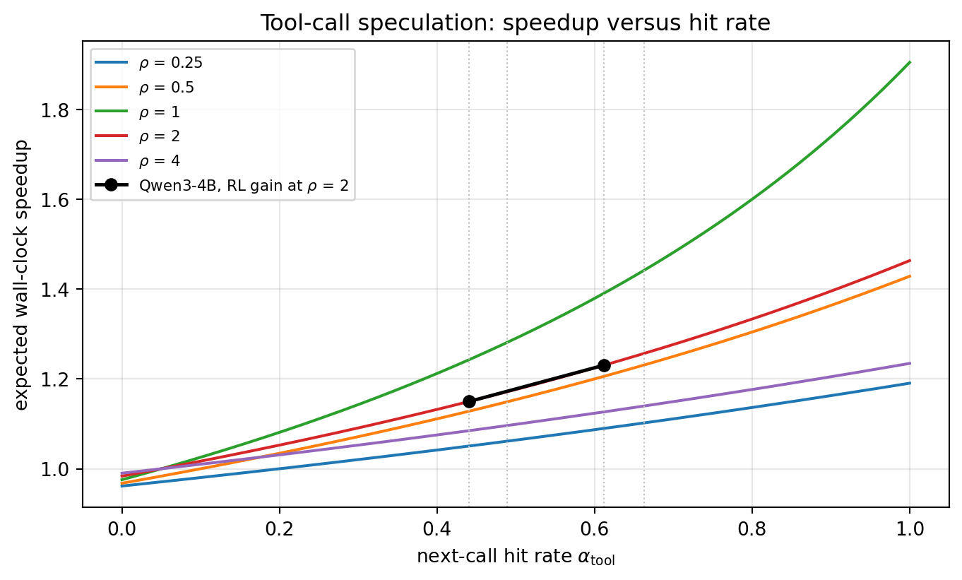
           setting  alpha  rho=0.25   rho=0.5     rho=1     rho=2     rho=4
   Qwen3-4B before  0.441      4.8%     11.4%     19.6%     13.0%      7.8%
    Qwen3-4B after  0.612      8.2%     17.1%     28.1%     18.7%     11.2%
 Qwen3.5-4B before  0.489      5.8%     13.0%     22.0%     14.6%      8.8%
  Qwen3.5-4B after  0.663      9.3%     18.8%     30.7%     20.4%     12.3%

closed form vs simulated 200k-turn trajectory
  alpha=0.441 rho=0.5  closed=1.1282  simulated=1.1283
  alpha=0.441 rho=2.0  closed=1.1499  simulated=1.1497
  alpha=0.612 rho=0.5  closed=1.2058  simulated=1.2054
  alpha=0.612 rho=2.0  closed=1.2305  simulated=1.2295
The table makes the shape of the win concrete. Benefit peaks near \(\rho = 1\), where a hit hides the tool completely inside the generation window, and decays for very slow tools because one turn of overlap can only absorb \(T_{\text{gen}}\) of waiting. That decay is the tool-level counterpart of the interior optimum in \(k\) from Section 3.5, and it motivates the same response: speculate further ahead. Guessing \(k\) calls deep multiplies hit probabilities, so depth pays only when the per-step \(\alpha_{\text{tool}}\) is high, which is precisely what the joint training buys. Whether the unit is a token, a block of tokens, or an entire tool invocation, the governing quantity never changes: the speedup is a function of the acceptance rate, and every worthwhile advance in speculative execution is an advance in aligning the proposer with the thing doing the verifying.
251.5 Production Code
In production you do not implement the accept-reject loop by hand. Mature open-source serving frameworks ship speculative decoding as a configuration flag, with optimized fused kernels, tree attention, paged key-value caches, and continuous batching already integrated. The free, widely used options are vLLM, Hugging Face Text Generation Inference (TGI), and NVIDIA TensorRT-LLM, plus the transformers library itself for quick experiments. The code in this section requires a GPU and large model weights, so it is shown rather than executed here. Each block is a faithful, runnable invocation.
251.5.1 Draft-model speculation in transformers
The simplest entry point is the assistant_model argument to generate, which performs exact speculative decoding with a smaller assistant. The draft and target must share a tokenizer.
# requires GPU and large model weights; not executed in this CPU build.
import torch
from transformers import AutoModelForCausalLM, AutoTokenizer

target_id = "meta-llama/Llama-3.1-8B-Instruct"
draft_id  = "meta-llama/Llama-3.2-1B-Instruct"   # same tokenizer family

tok = AutoTokenizer.from_pretrained(target_id)
target = AutoModelForCausalLM.from_pretrained(target_id, torch_dtype=torch.bfloat16, device_map="cuda")
draft  = AutoModelForCausalLM.from_pretrained(draft_id,  torch_dtype=torch.bfloat16, device_map="cuda")

prompt = "Explain why memory bandwidth dominates LLM inference latency."
inputs = tok(prompt, return_tensors="pt").to("cuda")

out = target.generate(
    **inputs,
    assistant_model=draft,        # turns on exact speculative decoding
    num_assistant_tokens=5,       # the block length k
    do_sample=True, temperature=0.7, max_new_tokens=256,
)
print(tok.decode(out[0], skip_special_tokens=True))
251.5.2 vLLM with a draft model
vLLM exposes speculation through the engine configuration. The output distribution is identical to non-speculative serving; only latency changes.
# requires GPU; not executed in this CPU build.
from vllm import LLM, SamplingParams

llm = LLM(
    model="meta-llama/Llama-3.1-70B-Instruct",
    speculative_config={
        "model": "meta-llama/Llama-3.2-1B-Instruct",
        "num_speculative_tokens": 5,
    },
    tensor_parallel_size=4,
)
params = SamplingParams(temperature=0.7, max_tokens=256)
print(llm.generate(["Summarize speculative decoding in two sentences."], params)[0].outputs[0].text)
251.5.3 EAGLE heads in vLLM
For self-contained speculation without a separate draft model, vLLM supports EAGLE and Medusa draft heads. Only the head checkpoint is extra; the base model is the target you already serve.
# requires GPU; not executed in this CPU build.
from vllm import LLM, SamplingParams

llm = LLM(
    model="meta-llama/Llama-3.1-8B-Instruct",
    speculative_config={
        "method": "eagle",
        "model": "yuhuili/EAGLE-LLaMA3.1-Instruct-8B",  # trained EAGLE head
        "num_speculative_tokens": 5,
    },
)
print(llm.generate(["Describe tree attention."], SamplingParams(max_tokens=128))[0].outputs[0].text)
251.5.4 A note on quantized drafts
A common production pattern is a quantized draft model to make the draft pass even cheaper. Libraries such as bitsandbytes provide 4-bit and 8-bit loading, but they require a GPU, so this is shown, not executed. Because verification is exact, a lossy quantized draft only affects the acceptance rate, never the output distribution.
# requires GPU and bitsandbytes; not executed in this CPU build.
from transformers import AutoModelForCausalLM, BitsAndBytesConfig
import torch

nf4 = BitsAndBytesConfig(load_in_4bit=True, bnb_4bit_compute_dtype=torch.bfloat16)
draft = AutoModelForCausalLM.from_pretrained(
    "meta-llama/Llama-3.2-1B-Instruct", quantization_config=nf4, device_map="cuda"
)
# Pass `draft` as assistant_model exactly as in Section 5.1.
251.6 Pitfalls and When to Use
Speculative decoding helps latency, not throughput at saturation. The free lunch comes from idle accelerator cycles at small batch sizes. When the server is already compute bound (large batches, high concurrency), the target forward pass is no longer cheap to widen, the extra draft work competes for the same compute, and speculation can reduce total throughput. Use it for latency-sensitive, low-to-moderate-concurrency serving, and measure under your real batching regime rather than assuming a benefit.
Acceptance rate is everything, and it is workload dependent. The speedup formula collapses toward one as \(\alpha\) falls. A draft that is well aligned on code may be poorly aligned on multilingual chat or long-context reasoning. Always measure \(\alpha\) on representative traffic, not a toy prompt, and prefer drafts trained or distilled from the same family as the target.
The draft must share the target’s tokenizer. Different tokenizers make the per-position probability comparison meaningless and break the acceptance test. This is a hard constraint for the vanilla method and a reason self-drafting variants such as Medusa and EAGLE are attractive.
Tune the block length k; do not hard-code it. As Section 3.5 showed, the optimal \(k\) depends on both \(\alpha\) and the draft-to-target cost ratio. Too large a block wastes draft passes on tokens that will be rejected. Adaptive block-length schemes that grow \(k\) after a run of accepts and shrink it after rejects are common and worthwhile.
Verify exactness in your stack, especially with sampling. The guarantee holds only if verification uses the same temperature, top-p, top-k, and logit processors as the target would have used alone. A mismatch between the draft’s and target’s sampling configuration silently breaks the residual-distribution math and biases the output. Greedy decoding is the easy case (accept iff the draft’s argmax equals the target’s); sampling needs the full accept-reject rule of Section 2.
Memory and complexity costs are real. You hold a second model (or extra heads) in memory, and tree-based variants add attention-mask bookkeeping. On memory-constrained hardware the draft model’s footprint can be the deciding factor against using a separate draft at all, which again favors lightweight head-based methods.
When these conditions are met, namely latency-bound serving, a well-aligned draft sharing the tokenizer, and a tuned block length, speculative decoding is one of the highest-leverage, lowest-risk optimizations available, because it is exact: you change only how fast tokens arrive, never which tokens they are.
251.7 References
- Leviathan, Y., Kalman, M., and Matias, Y. “Fast Inference from Transformers via Speculative Decoding.” International Conference on Machine Learning, 2023. https://arxiv.org/abs/2211.17192
- Chen, C., Borgeaud, S., Irving, G., Lespiau, J.-B., Sifre, L., and Jumper, J. “Accelerating Large Language Model Decoding with Speculative Sampling.” 2023. https://arxiv.org/abs/2302.01318
- Cai, T., Li, Y., Geng, Z., Peng, H., Lee, J. D., Chen, D., and Dao, T. “Medusa: Simple LLM Inference Acceleration Framework with Multiple Decoding Heads.” International Conference on Machine Learning, 2024. https://arxiv.org/abs/2401.10774
- Li, Y., Wei, F., Zhang, C., and Zhang, H. “EAGLE: Speculative Sampling Requires Rethinking Feature Uncertainty.” International Conference on Machine Learning, 2024. https://arxiv.org/abs/2401.15077
- Li, Y., Wei, F., Zhang, C., and Zhang, H. “EAGLE-2: Faster Inference of Language Models with Dynamic Draft Trees.” Conference on Empirical Methods in Natural Language Processing, 2024. https://arxiv.org/abs/2406.16858
- Stern, M., Shazeer, N., and Uszkoreit, J. “Blockwise Parallel Decoding for Deep Autoregressive Models.” Advances in Neural Information Processing Systems, 2018. https://arxiv.org/abs/1811.03115
- Xia, H., Yang, Z., Dong, Q., Wang, P., Li, Y., Ge, T., Liu, T., Li, W., and Sui, Z. “Unlocking Efficiency in Large Language Model Inference: A Survey of Speculative Decoding.” Findings of the Association for Computational Linguistics, 2024. https://arxiv.org/abs/2401.07851
- vLLM developers. “Speculative Decoding.” vLLM documentation. https://docs.vllm.ai/en/latest/features/spec_decode.html
- Ji, J., Liu, Y., An, L., Jain, R., Polatkan, G., Zhu, S., and Chang, S. “Speculate While You Reason: Teaching Agents to Predict Their Next Tool Call via Joint Agent-Speculator RL.” 2026. https://arxiv.org/abs/2607.25816