Two strings can mean the same thing while sharing almost no characters (“JPMorgan Chase & Co” and “JPM”), and two strings can share almost every character while meaning different things (“bán” means to sell in Vietnamese and “bàn” means table). Every system that deduplicates customers, links a news article to a company, matches a supplier invoice to a vendor master, or ranks web pages against an industry description has to decide, pair by pair, how similar two pieces of text are and whether that similarity is strong enough to act on.
This chapter treats the problem as a ladder. The bottom rung is lexical similarity: edit distance, set overlap, and TF-IDF cosine over words or character n-grams. These methods are cheap, transparent, and surprisingly strong for names. The middle rung is embedding similarity, where a neural encoder maps text to vectors so that paraphrases land close together. Sentence embeddings themselves are developed in Chapter 228 and Chapter 229, so here we focus on how to use them for matching, in particular the split between bi-encoders and cross-encoders. The top rung is entity matching (also called record linkage or entity resolution), where several fields are compared at once and a probabilistic model decides which record pairs refer to the same real-world entity. Throughout, we keep a multilingual lens and use Vietnamese as the running example, because its diacritics and multi-syllable words break naive pipelines in instructive ways.
230.1 Lexical Similarity
230.1.1 Edit distance
The Levenshtein distance\(d(a, b)\) between strings \(a\) and \(b\) is the minimum number of single-character insertions, deletions, and substitutions that turn \(a\) into \(b\) (Levenshtein 1966). It is computed by dynamic programming over a table \(D\) whose entry \(D_{i,j}\) is the distance between the first \(i\) characters of \(a\) and the first \(j\) characters of \(b\): \[
D_{i,j} = \min\big( D_{i-1,j} + 1,\ D_{i,j-1} + 1,\ D_{i-1,j-1} + \mathbb{1}[a_i \neq b_j] \big),
\qquad D_{i,0} = i,\ D_{0,j} = j .
\] The cost is \(O(|a|\,|b|)\) time. To compare strings of different lengths we normalize to a similarity in \([0, 1]\): \[
\text{sim}_{\text{lev}}(a, b) = 1 - \frac{d(a, b)}{\max(|a|, |b|)} .
\] The Damerau variant also counts a transposition of adjacent characters as one edit, which matters for typed data where “Nugyen” for “Nguyen” is common (Damerau 1964). For short person names the Jaro-Winkler similarity, designed at the US Census Bureau for exactly this setting, rewards agreement at the start of the string, where typing errors are rarer (Winkler 1990). Navarro (2001) surveys the algorithmic side of approximate string matching.
Edit distance is sensitive to word order. “Chase JPMorgan” and “JPMorgan Chase” are far apart in Levenshtein terms even though a human sees the same name. A cheap fix is token sort: lowercase, split into tokens, sort them alphabetically, rejoin, and only then compute the edit distance.
230.1.2 Set overlap and character n-grams
The Jaccard similarity of two sets is the size of their intersection over the size of their union (Jaccard 1912): \[
J(A, B) = \frac{|A \cap B|}{|A \cup B|} .
\] Applied to word sets it ignores order entirely. Applied to the set of character \(n\)-grams of a padded string (for \(n = 3\), “data” becomes ” da”, “dat”, “ata”, “ta”) it tolerates typos, since one wrong character destroys at most \(n\) of the \(n\)-grams and leaves the rest intact. Character n-grams also absorb morphology: “business” and “businesses” share most of their trigrams while being different word tokens.
230.1.3 TF-IDF cosine
Set overlap treats every token as equally informative. In a list of company names, the token “inc” carries almost no evidence while “netflix” carries a great deal. TF-IDF weighting captures this (Salton and Buckley 1988). For a term \(t\) in document \(d\) drawn from a collection of \(N\) documents, \[
w_{t,d} = \text{tf}(t, d) \cdot \log\frac{1 + N}{1 + \text{df}(t)} + \text{tf}(t, d),
\] where \(\text{df}(t)\) is the number of documents containing \(t\) (this is the smoothed form used by scikit-learn, which adds one to the logarithm). Each document becomes a vector \(\mathbf{w}_d\), normalized to unit length, and similarity is the cosine \[
\cos(\mathbf{w}_a, \mathbf{w}_b) = \frac{\mathbf{w}_a^\top \mathbf{w}_b}{\lVert \mathbf{w}_a\rVert\,\lVert \mathbf{w}_b \rVert} .
\] The “terms” can be words or character n-grams. TF-IDF over character n-grams within word boundaries is the workhorse of industrial company-name matching: it is a sparse matrix product, it scales to millions of names with approximate nearest-neighbor search over sparse vectors, and it inherits both the typo tolerance of n-grams and the down-weighting of boilerplate such as legal suffixes.
230.1.4 Comparing the lexical measures
The example below compares the measures on a small task: score three website snippets against a short industry description, as one would when classifying firms by the text on their websites. Everything is implemented from scratch except the TF-IDF vectorizer.
Code
import reimport timeimport unicodedataimport numpy as npimport pandas as pdimport matplotlib.pyplot as pltfrom sklearn.feature_extraction.text import TfidfVectorizerfrom sklearn.metrics.pairwise import cosine_similaritypd.set_option("display.width", 120)pd.set_option("display.max_columns", 12)def levenshtein(a: str, b: str) ->int:"""Edit distance by the two-row dynamic program."""iflen(a) <len(b): a, b = b, a prev =list(range(len(b) +1))for i, ca inenumerate(a, 1): cur = [i]for j, cb inenumerate(b, 1): cur.append(min(prev[j] +1, cur[j -1] +1, prev[j -1] + (ca != cb))) prev = curreturn prev[-1]def lev_sim(a: str, b: str) ->float:ifnot a andnot b:return1.0return1.0- levenshtein(a, b) /max(len(a), len(b))def char_ngrams(s: str, n: int=3) ->set: s =f" {s} "return {s[i:i + n] for i inrange(len(s) - n +1)}def jaccard(A: set, B: set) ->float:returnlen(A & B) /len(A | B) if (A | B) else1.0def tfidf_cos(query, docs, **kw): vec = TfidfVectorizer(**kw).fit([query] + docs)return cosine_similarity(vec.transform([query]), vec.transform(docs))[0]industry ="industry data warehouse and data for businesses"websites = ["We are the best business data seller in the country","We can give you the best warehouse for you in the country","Look no further for your warehouse needs",]q = industry.lower()rows = []for i, w inenumerate(websites): d = w.lower() rows.append({"site": f"site {i +1}","levenshtein": lev_sim(q, d),"jaccard_words": jaccard(set(q.split()), set(d.split())),"jaccard_char3": jaccard(char_ngrams(q), char_ngrams(d)), })lex = pd.DataFrame(rows).set_index("site")lex["tfidf_words"] = tfidf_cos(industry, websites, stop_words="english")lex["tfidf_char_wb"] = tfidf_cos(industry, websites, analyzer="char_wb", ngram_range=(2, 4))print(lex.round(3))print("\nbest site per measure:")print(lex.idxmax())
        levenshtein  jaccard_words  jaccard_char3  tfidf_words  tfidf_char_wb
site
site 1        0.216          0.071          0.213        0.286          0.413
site 2        0.281          0.143          0.192        0.143          0.223
site 3        0.234          0.182          0.169        0.119          0.191

best site per measure:
levenshtein      site 2
jaccard_words    site 3
jaccard_char3    site 1
tfidf_words      site 1
tfidf_char_wb    site 1
dtype: object
The measures disagree, and the disagreement is informative. Whole-string Levenshtein mostly reflects length and shared function words, so it is a poor choice for comparing sentences. Word-level TF-IDF with English stop words removed sees only exact token matches: “business” in the first snippet and “businesses” in the description are different tokens, so the first snippet gets credit only for “data”. The character n-gram variant links “business” and “businesses” through their shared n-grams. None of these methods knows that a “data seller” is closer to a “data warehouse” business than a physical “warehouse” is. That gap is what embeddings close, and we return to it below.
230.2 Multilingual Text: The Vietnamese Case
Lexical methods silently assume that equal-looking text is equal at the byte level and that whitespace separates words. Vietnamese violates both assumptions, and so do many other languages, so it is worth working through the details.
Diacritics and Unicode normalization. Vietnamese uses the Latin alphabet with a rich set of diacritics: vowel modifiers (ă, â, ê, ô, ơ, ư), the letter đ, and five tone marks. A character such as “ữ” can be stored as a single precomposed code point (Unicode Normalization Form C, NFC) or as a base letter followed by combining marks (Form D, NFD). The two encodings render identically and compare unequal. Text pasted from different keyboards, operating systems, and PDF extractors arrives in a mixture of both. Worse, many users type Vietnamese without any diacritics at all, so “dữ liệu” (data) also appears as “du lieu”.
Syllables versus words. Vietnamese writes one syllable per whitespace-delimited token, and most words are compounds of two or more syllables: “dữ liệu” (data), “công nghệ” (technology), “buôn bán” (trade). Splitting on whitespace therefore produces syllables, and a syllable such as “liệu” carries little meaning alone. Word segmenters such as VnCoreNLP (Vu et al. 2018) and the underthesea toolkit join syllables into words (“dữ_liệu”), and the Vietnamese language model PhoBERT expects word-segmented input (Nguyen and Nguyen 2020).
The next chunk demonstrates both problems and the standard fixes: NFC normalization, optional diacritic folding, syllable bigrams as a cheap stand-in for word segmentation, and character n-grams.
Code
def nfc(s: str) ->str:return unicodedata.normalize("NFC", s)def fold_vi(s: str) ->str:"""Strip Vietnamese diacritics: decompose, drop combining marks, map đ to d.""" s = unicodedata.normalize("NFD", s) s ="".join(ch for ch in s if unicodedata.category(ch) !="Mn")return s.replace("đ", "d").replace("Đ", "D")word ="dữ liệu"w_nfc, w_nfd = nfc(word), unicodedata.normalize("NFD", word)print("renders the same:", w_nfc, "|", w_nfd)print("equal as strings:", w_nfc == w_nfd, "| code points:", len(w_nfc), "vs", len(w_nfd))# The default TF-IDF token pattern treats combining marks as non-word characters,# so NFD text is shredded into fragments before any similarity is computed.analyzer = TfidfVectorizer().build_analyzer()print("NFC tokens:", analyzer(w_nfc))print("NFD tokens:", analyzer(w_nfd))print("folded :", fold_vi(word))# Folding is lossy: distinct words collapse onto one form.syllables = ["bán", "bàn", "bạn", "bản", "ban", "bận"]print("folding collisions:", {s: fold_vi(s) for s in syllables})
renders the same: dữ liệu | dữ liệu
equal as strings: False | code points: 7 vs 11
NFC tokens: ['dữ', 'liệu']
NFD tokens: ['du', 'lie']
folded    : du lieu
folding collisions: {'bán': 'ban', 'bàn': 'ban', 'bạn': 'ban', 'bản': 'ban', 'ban': 'ban', 'bận': 'ban'}
The NFD form is not merely different from the NFC form, it is tokenized into different pieces, so any similarity computed on mixed-normalization text is corrupted at the first step. The fix is mechanical: normalize every string to NFC at ingestion, before storage, hashing, or indexing.
Diacritic folding is a judgment call. It makes “du lieu” match “dữ liệu”, which is usually what a search box or a name matcher wants. It also merges sell, table, friend, copy, and busy into a single token, which destroys meaning for semantic tasks. A robust pattern is to index both forms and let the folded form contribute recall while the accented form contributes precision.
Now the comparison on Vietnamese text. The industry description is “Ngành nghề buôn bán dữ liệu” (the data trading business). Three website snippets are written with diacritics, and a fourth repeats the first one without diacritics, as many users would type it.
Code
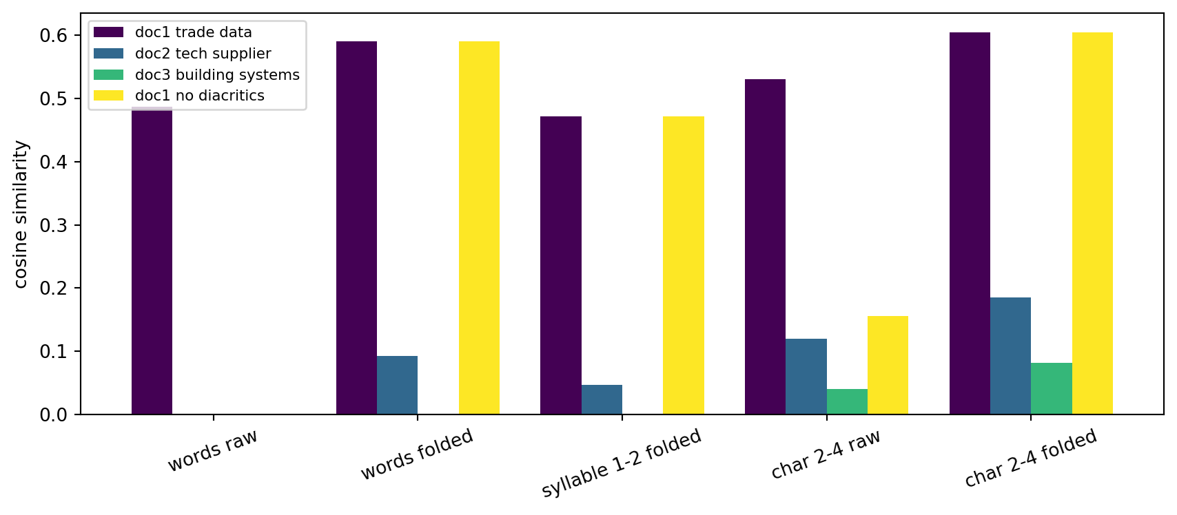
query_vi = nfc("Ngành nghề buôn bán dữ liệu")docs_vi = [nfc(s) for s in ["Chúng tôi buôn bán dữ liệu và công nghệ", # we trade data and technology"Bên cung cấp công nghệ", # technology supplier"Hiện tại chúng tôi đang phát triển hệ thống", # we are currently building systems"Chung toi buon ban du lieu va cong nghe", # doc 1 typed without diacritics]]configs = {"words raw": (lambda s: s.lower(), dict()),"words folded": (lambda s: fold_vi(s).lower(), dict()),"syllable 1-2 folded": (lambda s: fold_vi(s).lower(), dict(ngram_range=(1, 2))),"char 2-4 raw": (lambda s: s.lower(), dict(analyzer="char_wb", ngram_range=(2, 4))),"char 2-4 folded": (lambda s: fold_vi(s).lower(), dict(analyzer="char_wb", ngram_range=(2, 4))),}vi = pd.DataFrame( {name: tfidf_cos(prep(query_vi), [prep(d) for d in docs_vi], **kw)for name, (prep, kw) in configs.items()}, index=["doc1 trade data", "doc2 tech supplier", "doc3 building systems", "doc1 no diacritics"],)print(vi.round(3))
                       words raw  words folded  syllable 1-2 folded  char 2-4 raw  char 2-4 folded
doc1 trade data            0.487         0.591                0.472         0.530            0.605
doc2 tech supplier         0.000         0.093                0.047         0.120            0.185
doc3 building systems      0.000         0.000                0.000         0.041            0.081
doc1 no diacritics         0.000         0.591                0.472         0.156            0.605
Figure 230.1: TF-IDF cosine similarity between a Vietnamese industry description and four snippets under five preprocessing choices. Without folding, the unaccented copy of the best-matching snippet shares no word tokens with the query. Folding and character n-grams recover it.
The raw word model gives the unaccented copy of the best snippet a similarity of zero, since no syllable matches byte for byte. Character n-grams recover part of the match even without folding because unaccented letters such as “n”, “g”, and “h” still align. Folding recovers it completely and makes the accented and unaccented versions of the first snippet indistinguishable. Adding syllable bigrams rewards the query and snippet for sharing the two-syllable words “buôn bán” and “dữ liệu” as units, which is the cheap version of what a word segmenter provides.
The equivalent pipeline with a real word segmenter looks as follows. It is shown rather than executed because it requires the underthesea package and its data.
Code
# Requires: pip install underthesea (not executed here).from underthesea import word_tokenizesegmented = [word_tokenize(nfc(s), format="text") for s in [query_vi] + docs_vi]# e.g. "Ngành_nghề buôn_bán dữ_liệu": multi-syllable words become single tokensvec = TfidfVectorizer(token_pattern=r"[^\s]+").fit(segmented)print(cosine_similarity(vec.transform(segmented[:1]), vec.transform(segmented[1:])))
Note that the segmenter itself is trained on accented text. Run it on NFC-normalized input before folding, then fold the segmented tokens if needed.
230.3 Embedding Similarity: Bi-Encoders and Cross-Encoders
Lexical methods cannot know that “nhà cung cấp công nghệ” and “technology vendor” mean the same thing. Neural encoders can. Two architectures dominate.
A bi-encoder maps each text independently to a vector \(f_\theta(x) \in \mathbb{R}^k\) and scores a pair by cosine similarity, \[
s_{\text{bi}}(q, d) = \cos\big(f_\theta(q), f_\theta(d)\big).
\] Because documents are encoded once and stored, scoring a query against \(N\) documents costs one encoder pass plus a nearest-neighbor search. Sentence-BERT made this practical by fine-tuning BERT in a siamese configuration so that cosine similarity of pooled outputs is meaningful (Reimers and Gurevych 2019). Multilingual bi-encoders such as LaBSE (Feng et al. 2022) and BGE-M3 (Chen et al. 2024) place translations near each other, so a Vietnamese query can retrieve an English document.
A cross-encoder feeds the pair through the transformer jointly and outputs a score, \[
s_{\text{cross}}(q, d) = g_\phi\big([\texttt{CLS}]\ q\ [\texttt{SEP}]\ d\big),
\] so every token of \(q\) attends to every token of \(d\). Cross-encoders are more accurate on fine-grained distinctions (negation, swapped roles, numbers) but cost one full forward pass per pair, so they cannot search a large collection directly (Humeau et al. 2020). The standard production design is retrieve then rerank: a bi-encoder (often combined with a sparse lexical retriever such as BM25 or the char-gram TF-IDF above) retrieves the top \(k\) candidates, and a cross-encoder reorders only those \(k\).
Two practical warnings carry over from Chapter 228. First, a raw pretrained encoder that was never trained for similarity, such as the [CLS] vector of PhoBERT, gives poorly calibrated cosines, so use a model fine-tuned for sentence similarity or fine-tune one on in-domain pairs. Second, cosine scores are not probabilities and their scale differs across models, so thresholds must be chosen on labeled pairs for each model. The Massive Text Embedding Benchmark compares models across tasks and languages and is a sensible place to shortlist candidates, but it does not replace an in-domain evaluation (Muennighoff et al. 2023).
The code below shows the retrieve-then-rerank pattern with current multilingual models. It downloads several gigabytes of weights, so it is not executed in this book.
Code
# Requires sentence-transformers and a model download (not executed here).from sentence_transformers import SentenceTransformer, CrossEncoder, utilbi = SentenceTransformer("BAAI/bge-m3") # multilingual bi-encoderreranker = CrossEncoder("BAAI/bge-reranker-v2-m3") # multilingual cross-encodercorpus = docs_vi + ["We sell business data and analytics", "Restaurant in Da Nang"]corpus_emb = bi.encode(corpus, normalize_embeddings=True)q_emb = bi.encode(query_vi, normalize_embeddings=True)# Stage 1: cheap retrieval by cosine similarity over precomputed vectors.hits = util.semantic_search(q_emb, corpus_emb, top_k=4)[0]candidates = [corpus[h["corpus_id"]] for h in hits]# Stage 2: expensive joint scoring of only the retrieved candidates.scores = reranker.predict([(query_vi, c) for c in candidates])for c, s insorted(zip(candidates, scores), key=lambda t: -t[1]):print(f"{s:7.3f}{c}")
230.4 Name Matching
Company and person names are short, so the semantic machinery of embeddings adds less than it does for sentences, while the specific noise of names (typos, abbreviations, legal suffixes, reordered tokens, dropped diacritics) is exactly what lexical methods handle well. The experiment below generates noisy variants of ten well-known company names and asks each method to map every variant back to the right canonical name.
Code
rng = np.random.default_rng(1204)canonical = ["Apple Inc", "Google LLC", "Microsoft Corporation", "Amazon.com Inc","Meta Platforms Inc", "Netflix Inc", "Tesla Inc", "JPMorgan Chase & Co","Walmart Inc", "Procter & Gamble Co",]LEGAL =r"\b(inc|llc|corporation|corp|co|ltd|group|company)\b"def noisy_variant(name: str) ->str:"""Apply one or two realistic corruptions to a canonical name.""" ops = ["strip_legal", "lower", "typo", "shuffle", "abbrev", "and"] out = namefor op in rng.choice(ops, size=rng.integers(1, 3), replace=False):if op =="strip_legal": out = re.sub(LEGAL, "", out, flags=re.I).strip()elif op =="lower": out = out.lower()elif op =="typo"andlen(out) >4: i = rng.integers(1, len(out) -1) out = out[:i] + out[i +1:] if rng.random() <0.5else out[:i] + out[i +1] + out[i] + out[i +2:]elif op =="shuffle"andlen(out.split()) >1: toks = out.split() rng.shuffle(toks) out =" ".join(toks)elif op =="abbrev": out = out.replace("Corporation", "Corp").replace("Company", "Co")elif op =="and": out = out.replace("&", "and")return re.sub(r"\s+", " ", out).strip()truth = rng.integers(0, len(canonical), size=400)queries = [noisy_variant(canonical[t]) for t in truth]def normalize_name(s: str) ->str: s = fold_vi(s).lower().replace("&", " and ") s = re.sub(r"[^\w\s]", " ", s) s = re.sub(LEGAL, " ", s)return re.sub(r"\s+", " ", s).strip()def token_sort(s: str) ->str:return" ".join(sorted(s.split()))def argmax_match(score_fn):return np.array([np.argmax([score_fn(qr, c) for c in canonical]) for qr in queries])methods = {"levenshtein raw": lambda a, b: lev_sim(a, b),"levenshtein normalized": lambda a, b: lev_sim(normalize_name(a), normalize_name(b)),"token-sort normalized": lambda a, b: lev_sim(token_sort(normalize_name(a)), token_sort(normalize_name(b))),}results = {}for name, fn in methods.items(): t0 = time.perf_counter() pred = argmax_match(fn) results[name] = {"top1_accuracy": (pred == truth).mean(), "seconds": time.perf_counter() - t0}for name, kw, prep in [ ("tfidf words normalized", dict(), normalize_name), ("tfidf char_wb 2-3 raw", dict(analyzer="char_wb", ngram_range=(2, 3)), lambda s: s), ("tfidf char_wb 2-3 normalized", dict(analyzer="char_wb", ngram_range=(2, 3)), normalize_name),]: t0 = time.perf_counter() vec = TfidfVectorizer(**kw).fit([prep(c) for c in canonical]) S = cosine_similarity(vec.transform([prep(x) for x in queries]), vec.transform([prep(c) for c in canonical])) pred = S.argmax(axis=1) results[name] = {"top1_accuracy": (pred == truth).mean(), "seconds": time.perf_counter() - t0}print(pd.DataFrame(results).T.round(4).sort_values("top1_accuracy", ascending=False))
For edit distance, normalization (case, punctuation, legal suffixes) matters as much as the choice of function. Raw edit distance is hurt by token reordering and by legal suffixes that inflate or deflate length, and token sorting removes the reordering problem. Word-level TF-IDF is the weakest method here, because a single typo turns a distinctive token into one that matches nothing in the vocabulary. Character n-gram TF-IDF is competitive even on raw input and is also the fastest, because scoring every query against every candidate is a single sparse matrix product rather than a Python loop. That speed advantage grows with the size of the master list, which is why it is the default first stage for large name-matching systems.
230.5 Entity Matching and Record Linkage
Real records have several fields, and no single field is decisive. Two customer records with the same family name “Nguyễn” are weak evidence of a match, because a very large share of Vietnamese people carry that name. The same birth year and province are stronger evidence, and a rare given name stronger still. Record linkage formalizes how to combine such evidence. The classic reference is Christen (2012).
230.5.1 The Fellegi-Sunter model
Consider two files \(A\) and \(B\) and the set of all pairs \((a, b) \in A \times B\). Each pair is either a match (\(M\)) or a non-match (\(U\)). For each of \(K\) fields we compute a comparison outcome \(\gamma_k \in \{0, 1\}\) (agree or disagree, possibly after fuzzy comparison), giving a vector \(\boldsymbol{\gamma} = (\gamma_1, \dots, \gamma_K)\). Fellegi and Sunter (1969) define the m-probabilities and u-probabilities\[
m_k = P(\gamma_k = 1 \mid M), \qquad u_k = P(\gamma_k = 1 \mid U).
\] The \(m_k\) measure field reliability (how often true matches agree, which typos and data entry errors push below one). The \(u_k\) measure coincidental agreement (how often unrelated records agree, which is large for “Nguyễn” and small for a rare given name). Under conditional independence of fields given match status, the log-likelihood ratio of a comparison vector is a sum of per-field match weights: \[
W(\boldsymbol{\gamma}) = \sum_{k=1}^{K} \left[\gamma_k \log_2 \frac{m_k}{u_k} + (1 - \gamma_k) \log_2 \frac{1 - m_k}{1 - u_k}\right].
\] Agreement on a field adds a positive weight and disagreement subtracts. Fellegi and Sunter showed that the optimal decision rule, for given tolerated rates of false matches and false non-matches, uses two thresholds: declare a match when \(W > T_\mu\), a non-match when \(W < T_\lambda\), and send the pairs in between to clerical review.
The \(m_k\) and \(u_k\) are usually unknown. Because the comparison vectors come from a two-component mixture, they can be estimated without labels by the EM algorithm. With mixing proportion \(p = P(M)\) and the conditional independence assumption, the E-step computes for each pair \[
g(\boldsymbol{\gamma}) = \frac{p \prod_k m_k^{\gamma_k}(1 - m_k)^{1 - \gamma_k}}{p \prod_k m_k^{\gamma_k}(1 - m_k)^{1 - \gamma_k} + (1 - p) \prod_k u_k^{\gamma_k}(1 - u_k)^{1 - \gamma_k}},
\] and the M-step updates \(p\), \(m_k\), and \(u_k\) as \(g\)-weighted and \((1-g)\)-weighted agreement rates. Since only \(2^K\) distinct comparison vectors exist, EM runs on pattern counts and is instantaneous even for millions of pairs.
230.5.2 Blocking
Comparing all \(|A| \cdot |B|\) pairs is quadratic and wasteful, since almost all pairs are non-matches. Blocking compares only pairs that share a blocking key (Papadakis et al. 2020). Two metrics describe a blocking scheme. The reduction ratio is the fraction of the full comparison space that is skipped, and the pairs completeness is the fraction of true matches that survive blocking: \[
\text{RR} = 1 - \frac{|C|}{|A| \cdot |B|}, \qquad \text{PC} = \frac{|C \cap M|}{|M|},
\] where \(C\) is the set of candidate pairs. A match lost at blocking can never be recovered downstream, so PC is a hard ceiling on recall. Using a union of several blocking keys protects against errors in any one field.
230.5.3 A worked linkage of Vietnamese person records
We simulate two files of Vietnamese person records that overlap in a known subset of people. Each record holds a family name, middle name, given name, date of birth, and province. File \(B\) is noisier: half of its records were typed without diacritics, and some have typos in the given name, missing middle names, birth years off by one, day and month swapped, or a changed province.
|A| = 1500, |B| = 1500, true matches = 1000
      family middle  given  day  month  year     province
91      Trần    Văn     Đt   23      8  1978     Đồng Nai
75        Lê  Quang    Mai   28      7  1969  Hồ Chí Minh
1264  Nguyễn          Ngân   14      6  1993  Hồ Chí Minh
330     Pham    Duc  Quynh   27      4  2003    Hai Phong
1349   Huynh    Van  Hieeu   10      7  1982   Binh Duong
First, blocking. We compare three schemes: block on family name, block on birth year, and a union of two keys (birth year, or the first two letters of the folded given name). All keys are computed on folded, lowercased text so that diacritics never split a block.
                   candidate_pairs  reduction_ratio  pairs_completeness
scheme
family name                 420764           0.8130               1.000
birth year                   49775           0.9779               0.901
year OR given[:2]           134759           0.9401               0.994
Blocking on family name is a poor choice in Vietnamese data, and the reason is demographic rather than technical: the most common family names create a handful of enormous blocks, so the reduction ratio is low, while the scheme still misses nothing only because family names are rarely mistyped. Blocking on birth year alone gives a large reduction but loses every match whose year was recorded off by one. The union keeps most of the reduction while recovering matches that either key alone would drop.
Next, the comparison vectors and the EM fit of the Fellegi-Sunter model. Given names are compared with normalized Levenshtein similarity at a threshold, so a single typo still counts as agreement.
Code
cand = np.array(sorted(candidates))a_idx, b_idx = cand[:, 0], cand[:, 1]_lev_cache = {}def giv_agree(x, y, thr=0.75): key = (x, y)if key notin _lev_cache: _lev_cache[key] = lev_sim(x, y) >= thrreturn _lev_cache[key]G = np.column_stack([ A["fam_f"].to_numpy()[a_idx] == B["fam_f"].to_numpy()[b_idx], (A["mid_f"].to_numpy()[a_idx] == B["mid_f"].to_numpy()[b_idx]), [giv_agree(x, y) for x, y inzip(A["giv_f"].to_numpy()[a_idx], B["giv_f"].to_numpy()[b_idx])], A["year"].to_numpy()[a_idx] == B["year"].to_numpy()[b_idx], A["month"].to_numpy()[a_idx] == B["month"].to_numpy()[b_idx], A["day"].to_numpy()[a_idx] == B["day"].to_numpy()[b_idx], A["prov_f"].to_numpy()[a_idx] == B["prov_f"].to_numpy()[b_idx],]).astype(int)fields = ["family", "middle", "given", "year", "month", "day", "province"]K =len(fields)is_match = np.array([(a, b) in true_pairs for a, b in cand])# EM on the distinct comparison patterns (at most 2^7 = 128 of them).patterns, inverse, counts = np.unique(G, axis=0, return_inverse=True, return_counts=True)inverse = inverse.ravel()# Start u at the overall agreement rate (nearly every candidate is a non-match)# and m at a high common value.p, m, u =0.01, np.full(K, 0.9), G.mean(axis=0)for _ inrange(1000): lm = np.prod(m ** patterns * (1- m) ** (1- patterns), axis=1) lu = np.prod(u ** patterns * (1- u) ** (1- patterns), axis=1) g = p * lm / (p * lm + (1- p) * lu) p_new = (counts * g).sum() / counts.sum()# M-step with a pseudo-count of one agreement and one disagreement per class,# which keeps m and u off the boundary so that no weight becomes infinite. m_new = ((counts * g) @ patterns +1) / ((counts * g).sum() +2) u_new = ((counts * (1- g)) @ patterns +1) / ((counts * (1- g)).sum() +2) converged =abs(p_new - p) <1e-12and np.allclose(m_new, m) and np.allclose(u_new, u) p, m, u = p_new, m_new, u_newif converged:breakoracle_m = G[is_match].mean(axis=0)oracle_u = G[~is_match].mean(axis=0)params = pd.DataFrame({"m_EM": m, "m_true": oracle_m, "u_EM": u, "u_true": oracle_u,"agree_weight": np.log2(m / u),"disagree_weight": np.log2((1- m) / (1- u))}, index=fields)print(f"estimated match share among candidates p = {p:.5f} (true {is_match.mean():.5f})")print(params.round(3))W_pat = (patterns * np.log2(m / u) + (1- patterns) * np.log2((1- m) / (1- u))).sum(axis=1)W = W_pat[inverse]post = g[inverse] # posterior match probability for each candidate pair
estimated match share among candidates p = 0.00700 (true 0.00738)
           m_EM  m_true   u_EM  u_true  agree_weight  disagree_weight
family    0.999   1.000  0.191   0.190         2.389           -9.080
middle    0.799   0.791  0.080   0.079         3.328           -2.197
given     0.970   0.969  0.459   0.459         1.080           -4.150
year      0.905   0.906  0.366   0.365         1.308           -2.738
month     0.999   0.961  0.084   0.084         3.568           -9.526
day       0.999   0.961  0.035   0.035         4.819           -9.411
province  0.869   0.862  0.098   0.098         3.144           -2.780
The unsupervised estimates land close to the oracle values computed from the hidden labels, and the weights tell the domain story. Agreement on family name earns a modest weight because unrelated people share a family name so often. Agreement on day of birth earns a large weight because coincidental agreement is rare. Disagreement on province costs relatively little because people move, so \(m\) for province is well below one.
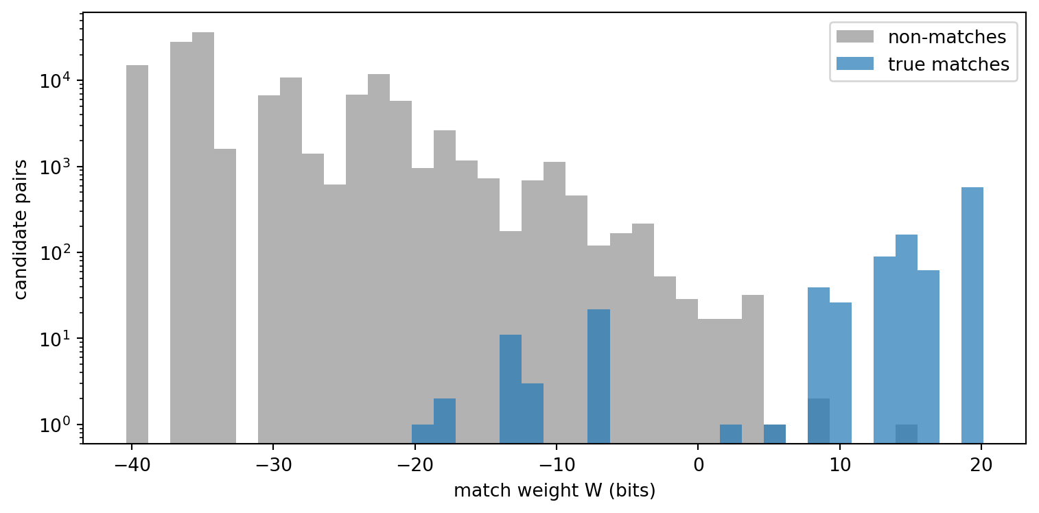
Two features of the table deserve a closer look. First, given name and birth year look like weak evidence, which seems wrong for a person-matching problem. It is an artifact of blocking. Every candidate pair was admitted because it agrees on birth year or on the start of the given name, so among candidates coincidental agreement on those two fields is common and their \(u\) values are inflated. Weights estimated after blocking are conditional on the blocking design and must be re-estimated whenever the keys change. Second, EM pushes \(m\) for day and month close to one, slightly above the oracle values. The few true matches whose day and month were swapped look, to the model, like non-matches, so the model learns that real matches essentially never disagree on those fields and then penalizes those pairs heavily. This is the conditional independence assumption failing in a specific, recognizable way: a swap makes two fields disagree together.
Figure 230.2: Distribution of Fellegi-Sunter match weights for true matches and non-matches among blocked candidate pairs (log scale on the vertical axis). Most true matches sit far to the right of the non-matches. The small group of true matches with negative weights consists of records whose day and month of birth were swapped, which the model penalizes twice.
230.5.4 Choosing thresholds and evaluating
A linkage is evaluated on pairs, with precision and recall defined relative to the true matches in the full comparison space, not only the candidates, so that blocking losses count against recall: \[
\text{precision} = \frac{|\hat{M} \cap M|}{|\hat{M}|}, \qquad \text{recall} = \frac{|\hat{M} \cap M|}{|M|}, \qquad F_1 = \frac{2 \cdot \text{precision} \cdot \text{recall}}{\text{precision} + \text{recall}} .
\] Accuracy is useless here, because declaring every pair a non-match is almost perfectly accurate.
Code
rows = []n_true =len(true_pairs)for T in [-4, 0, 4, 8, 12, 16]: pred = W > T tp = (pred & is_match).sum() prec = tp /max(pred.sum(), 1) rec = tp / n_true rows.append({"threshold_bits": T, "declared_matches": int(pred.sum()),"precision": prec, "recall": rec,"F1": 2* prec * rec /max(prec + rec, 1e-12)})print(pd.DataFrame(rows).set_index("threshold_bits").round(4))review = (post >0.05) & (post <0.95)print(f"\npairs in the clerical review band (0.05 < posterior < 0.95): {review.sum()}")print(f"share of those that are true matches: {is_match[review].mean():.3f}")
                declared_matches  precision  recall      F1
threshold_bits
-4                          1143     0.8355   0.955  0.8913
 0                          1025     0.9317   0.955  0.9432
 4                           990     0.9636   0.954  0.9588
 8                           956     0.9969   0.953  0.9744
 12                          889     0.9989   0.888  0.9402
 16                          575     1.0000   0.575  0.7302

pairs in the clerical review band (0.05 < posterior < 0.95): 117
share of those that are true matches: 0.573
Raising the threshold trades recall for precision in the familiar way. Recall can never exceed the pairs completeness of the blocking step. The posterior probability from EM gives a natural review band: pairs whose posterior sits between the extremes are few, and they are genuinely ambiguous, which is where a human reviewer or an expensive model adds the most value per decision.
230.6 Beyond the Classical Pipeline
The modern stack keeps the same skeleton (normalize, block, compare, decide) and upgrades individual stages. Deep entity matchers such as Ditto serialize each record into text and fine-tune a pretrained transformer as a cross-encoder over record pairs, with large gains on dirty and textual records (Li et al. 2020). Since 2023, generative LLMs have been used as zero-shot or few-shot matchers that read two serialized records and answer whether they match, and published comparisons show they can rival fine-tuned matchers on unseen entity types, at a much higher cost per pair (Peeters et al. 2025). Because cost per pair is the binding constraint, these models belong at the end of the pipeline: lexical or embedding blocking reduces the space, Fellegi-Sunter or a small classifier settles the clear cases, and the LLM or a human reviews the narrow ambiguous band.
230.7 Pitfalls and When to Use What
Normalize Unicode before anything else. Mixed NFC and NFD text corrupts tokens, hashes, and joins silently. Normalize to NFC at ingestion. Decide separately, per task, whether to fold diacritics, and when in doubt index both forms.
Do not fold diacritics for semantic tasks. Folding is a recall tool for names and search. For meaning, it merges distinct Vietnamese words and hurts any downstream model trained on accented text.
Treat syllable tokenization as a known approximation. Whitespace splits Vietnamese into syllables. Use a word segmenter, syllable bigrams, or character n-grams, and feed word-segmented text to models such as PhoBERT that expect it.
Thresholds are model specific. A cosine of 0.8 means different things for TF-IDF, for one embedding model, and for another. Calibrate thresholds on labeled pairs from your own data, and recalibrate when you change the model.
Blocking caps recall. Measure pairs completeness on a labeled sample before tuning the matcher. Use a union of keys on independent fields and avoid keys whose values are highly concentrated, such as Vietnamese family names.
The conditional independence assumption is wrong but useful. Fields such as province and phone area code are correlated, which makes Fellegi-Sunter overconfident. The ranking of pairs usually survives, but posterior probabilities should be recalibrated on labeled data before they are reported as probabilities.
Pairwise decisions must be reconciled. If \(a\) matches \(b\) and \(b\) matches \(c\), but \(a\) does not match \(c\), the pairwise output is inconsistent. Resolve it with a one-to-one assignment when each file has unique entities, or with clustering of the match graph for deduplication, and evaluate at the cluster level as well as the pair level.
Pick the cheapest method that works. For short names, normalized character n-gram TF-IDF is fast, transparent, and hard to beat. For sentences and cross-lingual text, use a fine-tuned bi-encoder for retrieval and a cross-encoder or LLM to rerank. For multi-field records, use blocking plus Fellegi-Sunter or a supervised classifier, and spend expensive models only on the ambiguous band.
230.8 References
Levenshtein, V. I. “Binary Codes Capable of Correcting Deletions, Insertions, and Reversals.” Soviet Physics Doklady 10(8), 1966, 707-710.
Damerau, F. J. “A Technique for Computer Detection and Correction of Spelling Errors.” Communications of the ACM 7(3), 1964, 171-176. https://doi.org/10.1145/363958.363994
Winkler, W. E. “String Comparator Metrics and Enhanced Decision Rules in the Fellegi-Sunter Model of Record Linkage.” Proceedings of the Section on Survey Research Methods, American Statistical Association, 1990, 354-359.
Navarro, G. “A Guided Tour to Approximate String Matching.” ACM Computing Surveys 33(1), 2001, 31-88. https://doi.org/10.1145/375360.375365
Jaccard, P. “The Distribution of the Flora in the Alpine Zone.” New Phytologist 11(2), 1912, 37-50. https://doi.org/10.1111/j.1469-8137.1912.tb05611.x
Salton, G. and Buckley, C. “Term-Weighting Approaches in Automatic Text Retrieval.” Information Processing and Management 24(5), 1988, 513-523. https://doi.org/10.1016/0306-4573(88)90021-0
Vu, T., Nguyen, D. Q., Nguyen, D. Q., Dras, M., and Johnson, M. “VnCoreNLP: A Vietnamese Natural Language Processing Toolkit.” Proceedings of NAACL-HLT 2018: Demonstrations, 2018, 56-60. https://doi.org/10.18653/v1/N18-5012
Nguyen, D. Q. and Nguyen, A. T. “PhoBERT: Pre-trained Language Models for Vietnamese.” Findings of the Association for Computational Linguistics: EMNLP 2020, 2020, 1037-1042. https://doi.org/10.18653/v1/2020.findings-emnlp.92
Reimers, N. and Gurevych, I. “Sentence-BERT: Sentence Embeddings using Siamese BERT-Networks.” Proceedings of EMNLP-IJCNLP 2019, 2019, 3982-3992. https://doi.org/10.18653/v1/D19-1410
Feng, F., Yang, Y., Cer, D., Arivazhagan, N., and Wang, W. “Language-agnostic BERT Sentence Embedding.” Proceedings of the 60th Annual Meeting of the Association for Computational Linguistics (Volume 1: Long Papers), 2022, 878-891. https://doi.org/10.18653/v1/2022.acl-long.62
Chen, J., Xiao, S., Zhang, P., Luo, K., Lian, D., and Liu, Z. “M3-Embedding: Multi-Linguality, Multi-Functionality, Multi-Granularity Text Embeddings Through Self-Knowledge Distillation.” Findings of the Association for Computational Linguistics: ACL 2024, 2024, 2318-2335. https://doi.org/10.18653/v1/2024.findings-acl.137
Humeau, S., Shuster, K., Lachaux, M.-A., and Weston, J. “Poly-encoders: Architectures and Pre-training Strategies for Fast and Accurate Multi-sentence Scoring.” International Conference on Learning Representations (ICLR), 2020. https://openreview.net/forum?id=SkxgnnNFvH
Muennighoff, N., Tazi, N., Magne, L., and Reimers, N. “MTEB: Massive Text Embedding Benchmark.” Proceedings of the 17th Conference of the European Chapter of the Association for Computational Linguistics, 2023, 2014-2037. https://doi.org/10.18653/v1/2023.eacl-main.148
Fellegi, I. P. and Sunter, A. B. “A Theory for Record Linkage.” Journal of the American Statistical Association 64(328), 1969, 1183-1210. https://doi.org/10.2307/2286061
Christen, P. Data Matching: Concepts and Techniques for Record Linkage, Entity Resolution, and Duplicate Detection. Springer, 2012. https://doi.org/10.1007/978-3-642-31164-2
Papadakis, G., Skoutas, D., Thanos, E., and Palpanas, T. “Blocking and Filtering Techniques for Entity Resolution: A Survey.” ACM Computing Surveys 53(2), 2020, Article 31. https://doi.org/10.1145/3377455
Li, Y., Li, J., Suhara, Y., Doan, A., and Tan, W.-C. “Deep Entity Matching with Pre-Trained Language Models.” Proceedings of the VLDB Endowment 14(1), 2020, 50-60. https://doi.org/10.14778/3421424.3421431
Peeters, R., Steiner, A., and Bizer, C. “Entity Matching using Large Language Models.” Proceedings of the 28th International Conference on Extending Database Technology (EDBT), 2025, 529-541. https://doi.org/10.48786/edbt.2025.42
How to cite this chapter
Nguyen, M. (2026). Semantic Text Similarity and Entity Matching. In AI in Action: A Reference for Artificial Intelligence. https://mikenguyen13.github.io/ai_in_action/1204-semantic-similarity-entity-matching.html
BibTeX
@incollection{nguyen2026aiinaction-1204semanticsimilarityentitymatching,
  author    = {Nguyen, Mike},
  title     = {{Semantic Text Similarity and Entity Matching}},
  booktitle = {{AI in Action: A Reference for Artificial Intelligence}},
  year      = {2026},
  url       = {https://mikenguyen13.github.io/ai_in_action/1204-semantic-similarity-entity-matching.html},
  note      = {Online book}
}
Source Code
# Semantic Text Similarity and Entity Matching {#sec-semantic-similarity-entity-matching}Two strings can mean the same thing while sharing almost no characters ("JPMorgan Chase & Co" and "JPM"), and two strings can share almost every character while meaning different things ("bán" means *to sell* in Vietnamese and "bàn" means *table*). Every system that deduplicates customers, links a news article to a company, matches a supplier invoice to a vendor master, or ranks web pages against an industry description has to decide, pair by pair, how similar two pieces of text are and whether that similarity is strong enough to act on.This chapter treats the problem as a ladder. The bottom rung is **lexical similarity**: edit distance, set overlap, and TF-IDF cosine over words or character n-grams. These methods are cheap, transparent, and surprisingly strong for names. The middle rung is **embedding similarity**, where a neural encoder maps text to vectors so that paraphrases land close together. Sentence embeddings themselves are developed in @sec-sentence-embeddings and @sec-sbert, so here we focus on how to *use* them for matching, in particular the split between bi-encoders and cross-encoders. The top rung is **entity matching** (also called record linkage or entity resolution), where several fields are compared at once and a probabilistic model decides which record pairs refer to the same real-world entity. Throughout, we keep a multilingual lens and use Vietnamese as the running example, because its diacritics and multi-syllable words break naive pipelines in instructive ways.## Lexical Similarity### Edit distanceThe **Levenshtein distance** $d(a, b)$ between strings $a$ and $b$ is the minimum number of single-character insertions, deletions, and substitutions that turn $a$ into $b$ (Levenshtein 1966). It is computed by dynamic programming over a table $D$ whose entry $D_{i,j}$ is the distance between the first $i$ characters of $a$ and the first $j$ characters of $b$:$$D_{i,j} = \min\big( D_{i-1,j} + 1,\ D_{i,j-1} + 1,\ D_{i-1,j-1} + \mathbb{1}[a_i \neq b_j] \big),\qquad D_{i,0} = i,\ D_{0,j} = j .$$The cost is $O(|a|\,|b|)$ time. To compare strings of different lengths we normalize to a similarity in $[0, 1]$:$$\text{sim}_{\text{lev}}(a, b) = 1 - \frac{d(a, b)}{\max(|a|, |b|)} .$$The Damerau variant also counts a transposition of adjacent characters as one edit, which matters for typed data where "Nugyen" for "Nguyen" is common (Damerau 1964). For short person names the **Jaro-Winkler** similarity, designed at the US Census Bureau for exactly this setting, rewards agreement at the start of the string, where typing errors are rarer (Winkler 1990). Navarro (2001) surveys the algorithmic side of approximate string matching.Edit distance is sensitive to word order. "Chase JPMorgan" and "JPMorgan Chase" are far apart in Levenshtein terms even though a human sees the same name. A cheap fix is **token sort**: lowercase, split into tokens, sort them alphabetically, rejoin, and only then compute the edit distance.### Set overlap and character n-gramsThe **Jaccard similarity** of two sets is the size of their intersection over the size of their union (Jaccard 1912):$$J(A, B) = \frac{|A \cap B|}{|A \cup B|} .$$Applied to word sets it ignores order entirely. Applied to the set of character $n$-grams of a padded string (for $n = 3$, "data" becomes " da", "dat", "ata", "ta ") it tolerates typos, since one wrong character destroys at most $n$ of the $n$-grams and leaves the rest intact. Character n-grams also absorb morphology: "business" and "businesses" share most of their trigrams while being different word tokens.### TF-IDF cosineSet overlap treats every token as equally informative. In a list of company names, the token "inc" carries almost no evidence while "netflix" carries a great deal. **TF-IDF** weighting captures this (Salton and Buckley 1988). For a term $t$ in document $d$ drawn from a collection of $N$ documents,$$w_{t,d} = \text{tf}(t, d) \cdot \log\frac{1 + N}{1 + \text{df}(t)} + \text{tf}(t, d),$$where $\text{df}(t)$ is the number of documents containing $t$ (this is the smoothed form used by scikit-learn, which adds one to the logarithm). Each document becomes a vector $\mathbf{w}_d$, normalized to unit length, and similarity is the cosine$$\cos(\mathbf{w}_a, \mathbf{w}_b) = \frac{\mathbf{w}_a^\top \mathbf{w}_b}{\lVert \mathbf{w}_a\rVert\,\lVert \mathbf{w}_b \rVert} .$$The "terms" can be words or character n-grams. TF-IDF over character n-grams within word boundaries is the workhorse of industrial company-name matching: it is a sparse matrix product, it scales to millions of names with approximate nearest-neighbor search over sparse vectors, and it inherits both the typo tolerance of n-grams and the down-weighting of boilerplate such as legal suffixes.### Comparing the lexical measuresThe example below compares the measures on a small task: score three website snippets against a short industry description, as one would when classifying firms by the text on their websites. Everything is implemented from scratch except the TF-IDF vectorizer.```{python}#| label: code-1204-lexicalimport reimport timeimport unicodedataimport numpy as npimport pandas as pdimport matplotlib.pyplot as pltfrom sklearn.feature_extraction.text import TfidfVectorizerfrom sklearn.metrics.pairwise import cosine_similaritypd.set_option("display.width", 120)pd.set_option("display.max_columns", 12)def levenshtein(a: str, b: str) ->int:"""Edit distance by the two-row dynamic program."""iflen(a) <len(b): a, b = b, a prev =list(range(len(b) +1))for i, ca inenumerate(a, 1): cur = [i]for j, cb inenumerate(b, 1): cur.append(min(prev[j] +1, cur[j -1] +1, prev[j -1] + (ca != cb))) prev = curreturn prev[-1]def lev_sim(a: str, b: str) ->float:ifnot a andnot b:return1.0return1.0- levenshtein(a, b) /max(len(a), len(b))def char_ngrams(s: str, n: int=3) ->set: s =f" {s} "return {s[i:i + n] for i inrange(len(s) - n +1)}def jaccard(A: set, B: set) ->float:returnlen(A & B) /len(A | B) if (A | B) else1.0def tfidf_cos(query, docs, **kw): vec = TfidfVectorizer(**kw).fit([query] + docs)return cosine_similarity(vec.transform([query]), vec.transform(docs))[0]industry ="industry data warehouse and data for businesses"websites = ["We are the best business data seller in the country","We can give you the best warehouse for you in the country","Look no further for your warehouse needs",]q = industry.lower()rows = []for i, w inenumerate(websites): d = w.lower() rows.append({"site": f"site {i +1}","levenshtein": lev_sim(q, d),"jaccard_words": jaccard(set(q.split()), set(d.split())),"jaccard_char3": jaccard(char_ngrams(q), char_ngrams(d)), })lex = pd.DataFrame(rows).set_index("site")lex["tfidf_words"] = tfidf_cos(industry, websites, stop_words="english")lex["tfidf_char_wb"] = tfidf_cos(industry, websites, analyzer="char_wb", ngram_range=(2, 4))print(lex.round(3))print("\nbest site per measure:")print(lex.idxmax())```The measures disagree, and the disagreement is informative. Whole-string Levenshtein mostly reflects length and shared function words, so it is a poor choice for comparing sentences. Word-level TF-IDF with English stop words removed sees only exact token matches: "business" in the first snippet and "businesses" in the description are different tokens, so the first snippet gets credit only for "data". The character n-gram variant links "business" and "businesses" through their shared n-grams. None of these methods knows that a "data seller" is closer to a "data warehouse" business than a physical "warehouse" is. That gap is what embeddings close, and we return to it below.## Multilingual Text: The Vietnamese CaseLexical methods silently assume that equal-looking text is equal at the byte level and that whitespace separates words. Vietnamese violates both assumptions, and so do many other languages, so it is worth working through the details.**Diacritics and Unicode normalization.** Vietnamese uses the Latin alphabet with a rich set of diacritics: vowel modifiers (ă, â, ê, ô, ơ, ư), the letter đ, and five tone marks. A character such as "ữ" can be stored as a single precomposed code point (Unicode Normalization Form C, NFC) or as a base letter followed by combining marks (Form D, NFD). The two encodings render identically and compare unequal. Text pasted from different keyboards, operating systems, and PDF extractors arrives in a mixture of both. Worse, many users type Vietnamese without any diacritics at all, so "dữ liệu" (data) also appears as "du lieu".**Syllables versus words.** Vietnamese writes one *syllable* per whitespace-delimited token, and most words are compounds of two or more syllables: "dữ liệu" (data), "công nghệ" (technology), "buôn bán" (trade). Splitting on whitespace therefore produces syllables, and a syllable such as "liệu" carries little meaning alone. Word segmenters such as VnCoreNLP (Vu et al. 2018) and the underthesea toolkit join syllables into words ("dữ_liệu"), and the Vietnamese language model PhoBERT expects word-segmented input (Nguyen and Nguyen 2020).The next chunk demonstrates both problems and the standard fixes: NFC normalization, optional diacritic folding, syllable bigrams as a cheap stand-in for word segmentation, and character n-grams.```{python}#| label: code-1204-vietnamese-normalizationdef nfc(s: str) ->str:return unicodedata.normalize("NFC", s)def fold_vi(s: str) ->str:"""Strip Vietnamese diacritics: decompose, drop combining marks, map đ to d.""" s = unicodedata.normalize("NFD", s) s ="".join(ch for ch in s if unicodedata.category(ch) !="Mn")return s.replace("đ", "d").replace("Đ", "D")word ="dữ liệu"w_nfc, w_nfd = nfc(word), unicodedata.normalize("NFD", word)print("renders the same:", w_nfc, "|", w_nfd)print("equal as strings:", w_nfc == w_nfd, "| code points:", len(w_nfc), "vs", len(w_nfd))# The default TF-IDF token pattern treats combining marks as non-word characters,# so NFD text is shredded into fragments before any similarity is computed.analyzer = TfidfVectorizer().build_analyzer()print("NFC tokens:", analyzer(w_nfc))print("NFD tokens:", analyzer(w_nfd))print("folded :", fold_vi(word))# Folding is lossy: distinct words collapse onto one form.syllables = ["bán", "bàn", "bạn", "bản", "ban", "bận"]print("folding collisions:", {s: fold_vi(s) for s in syllables})```The NFD form is not merely different from the NFC form, it is tokenized into different pieces, so any similarity computed on mixed-normalization text is corrupted at the first step. The fix is mechanical: normalize every string to NFC at ingestion, before storage, hashing, or indexing.Diacritic folding is a judgment call. It makes "du lieu" match "dữ liệu", which is usually what a search box or a name matcher wants. It also merges *sell*, *table*, *friend*, *copy*, and *busy* into a single token, which destroys meaning for semantic tasks. A robust pattern is to index both forms and let the folded form contribute recall while the accented form contributes precision.Now the comparison on Vietnamese text. The industry description is "Ngành nghề buôn bán dữ liệu" (the data trading business). Three website snippets are written with diacritics, and a fourth repeats the first one without diacritics, as many users would type it.```{python}#| label: code-1204-vietnamese-similarityquery_vi = nfc("Ngành nghề buôn bán dữ liệu")docs_vi = [nfc(s) for s in ["Chúng tôi buôn bán dữ liệu và công nghệ", # we trade data and technology"Bên cung cấp công nghệ", # technology supplier"Hiện tại chúng tôi đang phát triển hệ thống", # we are currently building systems"Chung toi buon ban du lieu va cong nghe", # doc 1 typed without diacritics]]configs = {"words raw": (lambda s: s.lower(), dict()),"words folded": (lambda s: fold_vi(s).lower(), dict()),"syllable 1-2 folded": (lambda s: fold_vi(s).lower(), dict(ngram_range=(1, 2))),"char 2-4 raw": (lambda s: s.lower(), dict(analyzer="char_wb", ngram_range=(2, 4))),"char 2-4 folded": (lambda s: fold_vi(s).lower(), dict(analyzer="char_wb", ngram_range=(2, 4))),}vi = pd.DataFrame( {name: tfidf_cos(prep(query_vi), [prep(d) for d in docs_vi], **kw)for name, (prep, kw) in configs.items()}, index=["doc1 trade data", "doc2 tech supplier", "doc3 building systems", "doc1 no diacritics"],)print(vi.round(3))``````{python}#| label: fig-1204-vietnamese#| fig-cap: "TF-IDF cosine similarity between a Vietnamese industry description and four snippets under five preprocessing choices. Without folding, the unaccented copy of the best-matching snippet shares no word tokens with the query. Folding and character n-grams recover it."fig, ax = plt.subplots(figsize=(9, 4))vi.T.plot(kind="bar", ax=ax, width=0.8, colormap="viridis")ax.set_ylabel("cosine similarity")ax.set_xlabel("")ax.tick_params(axis="x", rotation=20)ax.legend(fontsize=8, loc="upper left")fig.tight_layout()plt.show()```The raw word model gives the unaccented copy of the best snippet a similarity of zero, since no syllable matches byte for byte. Character n-grams recover part of the match even without folding because unaccented letters such as "n", "g", and "h" still align. Folding recovers it completely and makes the accented and unaccented versions of the first snippet indistinguishable. Adding syllable bigrams rewards the query and snippet for sharing the two-syllable words "buôn bán" and "dữ liệu" as units, which is the cheap version of what a word segmenter provides.The equivalent pipeline with a real word segmenter looks as follows. It is shown rather than executed because it requires the underthesea package and its data.```{python}#| eval: false# Requires: pip install underthesea (not executed here).from underthesea import word_tokenizesegmented = [word_tokenize(nfc(s), format="text") for s in [query_vi] + docs_vi]# e.g. "Ngành_nghề buôn_bán dữ_liệu": multi-syllable words become single tokensvec = TfidfVectorizer(token_pattern=r"[^\s]+").fit(segmented)print(cosine_similarity(vec.transform(segmented[:1]), vec.transform(segmented[1:])))```Note that the segmenter itself is trained on accented text. Run it on NFC-normalized input *before* folding, then fold the segmented tokens if needed.## Embedding Similarity: Bi-Encoders and Cross-EncodersLexical methods cannot know that "nhà cung cấp công nghệ" and "technology vendor" mean the same thing. Neural encoders can. Two architectures dominate.A **bi-encoder** maps each text independently to a vector $f_\theta(x) \in \mathbb{R}^k$ and scores a pair by cosine similarity,$$s_{\text{bi}}(q, d) = \cos\big(f_\theta(q), f_\theta(d)\big).$$Because documents are encoded once and stored, scoring a query against $N$ documents costs one encoder pass plus a nearest-neighbor search. Sentence-BERT made this practical by fine-tuning BERT in a siamese configuration so that cosine similarity of pooled outputs is meaningful (Reimers and Gurevych 2019). Multilingual bi-encoders such as LaBSE (Feng et al. 2022) and BGE-M3 (Chen et al. 2024) place translations near each other, so a Vietnamese query can retrieve an English document.A **cross-encoder** feeds the pair through the transformer jointly and outputs a score,$$s_{\text{cross}}(q, d) = g_\phi\big([\texttt{CLS}]\ q\ [\texttt{SEP}]\ d\big),$$so every token of $q$ attends to every token of $d$. Cross-encoders are more accurate on fine-grained distinctions (negation, swapped roles, numbers) but cost one full forward pass *per pair*, so they cannot search a large collection directly (Humeau et al. 2020). The standard production design is **retrieve then rerank**: a bi-encoder (often combined with a sparse lexical retriever such as BM25 or the char-gram TF-IDF above) retrieves the top $k$ candidates, and a cross-encoder reorders only those $k$.Two practical warnings carry over from @sec-sentence-embeddings. First, a raw pretrained encoder that was never trained for similarity, such as the `[CLS]` vector of PhoBERT, gives poorly calibrated cosines, so use a model fine-tuned for sentence similarity or fine-tune one on in-domain pairs. Second, cosine scores are not probabilities and their scale differs across models, so thresholds must be chosen on labeled pairs for each model. The Massive Text Embedding Benchmark compares models across tasks and languages and is a sensible place to shortlist candidates, but it does not replace an in-domain evaluation (Muennighoff et al. 2023).The code below shows the retrieve-then-rerank pattern with current multilingual models. It downloads several gigabytes of weights, so it is not executed in this book.```{python}#| eval: false# Requires sentence-transformers and a model download (not executed here).from sentence_transformers import SentenceTransformer, CrossEncoder, utilbi = SentenceTransformer("BAAI/bge-m3") # multilingual bi-encoderreranker = CrossEncoder("BAAI/bge-reranker-v2-m3") # multilingual cross-encodercorpus = docs_vi + ["We sell business data and analytics", "Restaurant in Da Nang"]corpus_emb = bi.encode(corpus, normalize_embeddings=True)q_emb = bi.encode(query_vi, normalize_embeddings=True)# Stage 1: cheap retrieval by cosine similarity over precomputed vectors.hits = util.semantic_search(q_emb, corpus_emb, top_k=4)[0]candidates = [corpus[h["corpus_id"]] for h in hits]# Stage 2: expensive joint scoring of only the retrieved candidates.scores = reranker.predict([(query_vi, c) for c in candidates])for c, s insorted(zip(candidates, scores), key=lambda t: -t[1]):print(f"{s:7.3f}{c}")```## Name MatchingCompany and person names are short, so the semantic machinery of embeddings adds less than it does for sentences, while the specific noise of names (typos, abbreviations, legal suffixes, reordered tokens, dropped diacritics) is exactly what lexical methods handle well. The experiment below generates noisy variants of ten well-known company names and asks each method to map every variant back to the right canonical name.```{python}#| label: code-1204-company-namesrng = np.random.default_rng(1204)canonical = ["Apple Inc", "Google LLC", "Microsoft Corporation", "Amazon.com Inc","Meta Platforms Inc", "Netflix Inc", "Tesla Inc", "JPMorgan Chase & Co","Walmart Inc", "Procter & Gamble Co",]LEGAL =r"\b(inc|llc|corporation|corp|co|ltd|group|company)\b"def noisy_variant(name: str) ->str:"""Apply one or two realistic corruptions to a canonical name.""" ops = ["strip_legal", "lower", "typo", "shuffle", "abbrev", "and"] out = namefor op in rng.choice(ops, size=rng.integers(1, 3), replace=False):if op =="strip_legal": out = re.sub(LEGAL, "", out, flags=re.I).strip()elif op =="lower": out = out.lower()elif op =="typo"andlen(out) >4: i = rng.integers(1, len(out) -1) out = out[:i] + out[i +1:] if rng.random() <0.5else out[:i] + out[i +1] + out[i] + out[i +2:]elif op =="shuffle"andlen(out.split()) >1: toks = out.split() rng.shuffle(toks) out =" ".join(toks)elif op =="abbrev": out = out.replace("Corporation", "Corp").replace("Company", "Co")elif op =="and": out = out.replace("&", "and")return re.sub(r"\s+", " ", out).strip()truth = rng.integers(0, len(canonical), size=400)queries = [noisy_variant(canonical[t]) for t in truth]def normalize_name(s: str) ->str: s = fold_vi(s).lower().replace("&", " and ") s = re.sub(r"[^\w\s]", " ", s) s = re.sub(LEGAL, " ", s)return re.sub(r"\s+", " ", s).strip()def token_sort(s: str) ->str:return" ".join(sorted(s.split()))def argmax_match(score_fn):return np.array([np.argmax([score_fn(qr, c) for c in canonical]) for qr in queries])methods = {"levenshtein raw": lambda a, b: lev_sim(a, b),"levenshtein normalized": lambda a, b: lev_sim(normalize_name(a), normalize_name(b)),"token-sort normalized": lambda a, b: lev_sim(token_sort(normalize_name(a)), token_sort(normalize_name(b))),}results = {}for name, fn in methods.items(): t0 = time.perf_counter() pred = argmax_match(fn) results[name] = {"top1_accuracy": (pred == truth).mean(), "seconds": time.perf_counter() - t0}for name, kw, prep in [ ("tfidf words normalized", dict(), normalize_name), ("tfidf char_wb 2-3 raw", dict(analyzer="char_wb", ngram_range=(2, 3)), lambda s: s), ("tfidf char_wb 2-3 normalized", dict(analyzer="char_wb", ngram_range=(2, 3)), normalize_name),]: t0 = time.perf_counter() vec = TfidfVectorizer(**kw).fit([prep(c) for c in canonical]) S = cosine_similarity(vec.transform([prep(x) for x in queries]), vec.transform([prep(c) for c in canonical])) pred = S.argmax(axis=1) results[name] = {"top1_accuracy": (pred == truth).mean(), "seconds": time.perf_counter() - t0}print(pd.DataFrame(results).T.round(4).sort_values("top1_accuracy", ascending=False))```For edit distance, normalization (case, punctuation, legal suffixes) matters as much as the choice of function. Raw edit distance is hurt by token reordering and by legal suffixes that inflate or deflate length, and token sorting removes the reordering problem. Word-level TF-IDF is the weakest method here, because a single typo turns a distinctive token into one that matches nothing in the vocabulary. Character n-gram TF-IDF is competitive even on raw input and is also the fastest, because scoring every query against every candidate is a single sparse matrix product rather than a Python loop. That speed advantage grows with the size of the master list, which is why it is the default first stage for large name-matching systems.## Entity Matching and Record LinkageReal records have several fields, and no single field is decisive. Two customer records with the same family name "Nguyễn" are weak evidence of a match, because a very large share of Vietnamese people carry that name. The same birth year and province are stronger evidence, and a rare given name stronger still. **Record linkage** formalizes how to combine such evidence. The classic reference is Christen (2012).### The Fellegi-Sunter modelConsider two files $A$ and $B$ and the set of all pairs $(a, b) \in A \times B$. Each pair is either a match ($M$) or a non-match ($U$). For each of $K$ fields we compute a comparison outcome $\gamma_k \in \{0, 1\}$ (agree or disagree, possibly after fuzzy comparison), giving a vector $\boldsymbol{\gamma} = (\gamma_1, \dots, \gamma_K)$. Fellegi and Sunter (1969) define the **m-probabilities** and **u-probabilities**$$m_k = P(\gamma_k = 1 \mid M), \qquad u_k = P(\gamma_k = 1 \mid U).$$The $m_k$ measure field reliability (how often true matches agree, which typos and data entry errors push below one). The $u_k$ measure coincidental agreement (how often unrelated records agree, which is large for "Nguyễn" and small for a rare given name). Under conditional independence of fields given match status, the log-likelihood ratio of a comparison vector is a sum of per-field **match weights**:$$W(\boldsymbol{\gamma}) = \sum_{k=1}^{K} \left[\gamma_k \log_2 \frac{m_k}{u_k} + (1 - \gamma_k) \log_2 \frac{1 - m_k}{1 - u_k}\right].$$Agreement on a field adds a positive weight and disagreement subtracts. Fellegi and Sunter showed that the optimal decision rule, for given tolerated rates of false matches and false non-matches, uses two thresholds: declare a match when $W > T_\mu$, a non-match when $W < T_\lambda$, and send the pairs in between to clerical review.The $m_k$ and $u_k$ are usually unknown. Because the comparison vectors come from a two-component mixture, they can be estimated without labels by the EM algorithm. With mixing proportion $p = P(M)$ and the conditional independence assumption, the E-step computes for each pair$$g(\boldsymbol{\gamma}) = \frac{p \prod_k m_k^{\gamma_k}(1 - m_k)^{1 - \gamma_k}}{p \prod_k m_k^{\gamma_k}(1 - m_k)^{1 - \gamma_k} + (1 - p) \prod_k u_k^{\gamma_k}(1 - u_k)^{1 - \gamma_k}},$$and the M-step updates $p$, $m_k$, and $u_k$ as $g$-weighted and $(1-g)$-weighted agreement rates. Since only $2^K$ distinct comparison vectors exist, EM runs on pattern counts and is instantaneous even for millions of pairs.### BlockingComparing all $|A| \cdot |B|$ pairs is quadratic and wasteful, since almost all pairs are non-matches. **Blocking** compares only pairs that share a blocking key (Papadakis et al. 2020). Two metrics describe a blocking scheme. The **reduction ratio** is the fraction of the full comparison space that is skipped, and the **pairs completeness** is the fraction of true matches that survive blocking:$$\text{RR} = 1 - \frac{|C|}{|A| \cdot |B|}, \qquad \text{PC} = \frac{|C \cap M|}{|M|},$$where $C$ is the set of candidate pairs. A match lost at blocking can never be recovered downstream, so PC is a hard ceiling on recall. Using a union of several blocking keys protects against errors in any one field.### A worked linkage of Vietnamese person recordsWe simulate two files of Vietnamese person records that overlap in a known subset of people. Each record holds a family name, middle name, given name, date of birth, and province. File $B$ is noisier: half of its records were typed without diacritics, and some have typos in the given name, missing middle names, birth years off by one, day and month swapped, or a changed province.```{python}#| label: code-1204-simulate-recordsrng = np.random.default_rng(42)FAMILY = ["Nguyễn", "Trần", "Lê", "Phạm", "Hoàng", "Huỳnh", "Phan", "Vũ","Võ", "Đặng", "Bùi", "Đỗ", "Hồ", "Ngô", "Dương", "Lý"]fam_w = np.array([38, 11, 9.5, 7, 5, 5, 4.5, 3.9, 3.9, 2.1, 2, 1.4, 1.3, 1.3, 1, 0.5])MIDDLE = ["Văn", "Thị", "Hữu", "Đức", "Minh", "Ngọc", "Thanh", "Quang", "Xuân", "Hoài"]GIVEN = ["An", "Bình", "Châu", "Dũng", "Giang", "Hà", "Hải", "Hạnh", "Hiếu", "Hoa","Hùng", "Hương", "Khánh", "Lan", "Linh", "Long", "Mai", "Nam", "Ngân", "Nhung","Phong", "Phúc", "Phương", "Quân", "Quỳnh", "Sơn", "Tâm", "Thảo", "Thắng", "Trang","Trung", "Tuấn", "Uyên", "Vân", "Việt", "Vy", "Yến", "Khoa", "Đạt", "Duy"]PROVINCES = ["Hà Nội", "Hồ Chí Minh", "Đà Nẵng", "Hải Phòng", "Cần Thơ","Huế", "Nghệ An", "Thanh Hóa", "Bình Dương", "Đồng Nai"]n_people =2000people = pd.DataFrame({"pid": np.arange(n_people),"family": rng.choice(FAMILY, n_people, p=fam_w / fam_w.sum()),"middle": rng.choice(MIDDLE, n_people),"given": rng.choice(GIVEN, n_people),"year": rng.integers(1960, 2006, n_people),"month": rng.integers(1, 13, n_people),"day": rng.integers(1, 29, n_people),"province": rng.choice(PROVINCES, n_people),})A = people.iloc[:1500].reset_index(drop=True) # people 0..1499B = people.iloc[500:].reset_index(drop=True).copy() # people 500..1999, overlap 1000def typo(s: str) ->str: i = rng.integers(0, len(s)) kind = rng.integers(0, 3)if kind ==0andlen(s) >2:return s[:i] + s[i +1:] # deletionif kind ==1:return s[:i] + rng.choice(list("aeiouhnt")) + s[i +1:] # substitutionreturn s[:i] + s[i] + s[i:] # duplicationnB =len(B)B["given"] = [typo(g) if r <0.15else g for g, r inzip(B["given"], rng.random(nB))]B.loc[rng.random(nB) <0.20, "middle"] =""off = rng.random(nB) <0.10B.loc[off, "year"] += rng.choice([-1, 1], off.sum())# Day and month swapped (a dd/mm versus mm/dd confusion), possible only when day <= 12.swap = (rng.random(nB) <0.10) & (B["day"] <=12)B.loc[swap, ["day", "month"]] = B.loc[swap, ["month", "day"]].to_numpy()moved = rng.random(nB) <0.15B.loc[moved, "province"] = rng.choice(PROVINCES, moved.sum())no_marks = rng.random(nB) <0.5for col in ["family", "middle", "given", "province"]: B.loc[no_marks, col] = B.loc[no_marks, col].map(fold_vi)true_pairs =set(zip(A.index[A.pid >=500], B.index[B.pid <=1499]))print(f"|A| = {len(A)}, |B| = {len(B)}, true matches = {len(true_pairs)}")print(B.sample(5, random_state=1)[["family", "middle", "given", "day", "month", "year", "province"]])```First, blocking. We compare three schemes: block on family name, block on birth year, and a union of two keys (birth year, or the first two letters of the folded given name). All keys are computed on folded, lowercased text so that diacritics never split a block.```{python}#| label: code-1204-blockingfor df in (A, B): df["fam_f"] = df["family"].map(lambda s: fold_vi(s).lower()) df["mid_f"] = df["middle"].map(lambda s: fold_vi(s).lower()) df["giv_f"] = df["given"].map(lambda s: fold_vi(s).lower()) df["prov_f"] = df["province"].map(lambda s: fold_vi(s).lower()) df["giv2"] = df["giv_f"].str[:2]full_space =len(A) *len(B)ia = A.reset_index().rename(columns={"index": "ia"})ib = B.reset_index().rename(columns={"index": "ib"})def block_pairs(key):return ia[["ia", key]].merge(ib[["ib", key]], on=key)[["ia", "ib"]]def block_report(pairs, label): cand =set(map(tuple, pairs.to_numpy()))return {"scheme": label, "candidate_pairs": len(cand),"reduction_ratio": 1-len(cand) / full_space,"pairs_completeness": len(cand & true_pairs) /len(true_pairs)}, candreports = []for key, label in [("fam_f", "family name"), ("year", "birth year")]: rep, _ = block_report(block_pairs(key), label) reports.append(rep)union = pd.concat([block_pairs("year"), block_pairs("giv2")]).drop_duplicates()rep, candidates = block_report(union, "year OR given[:2]")reports.append(rep)print(pd.DataFrame(reports).set_index("scheme").round(4))```Blocking on family name is a poor choice in Vietnamese data, and the reason is demographic rather than technical: the most common family names create a handful of enormous blocks, so the reduction ratio is low, while the scheme still misses nothing only because family names are rarely mistyped. Blocking on birth year alone gives a large reduction but loses every match whose year was recorded off by one. The union keeps most of the reduction while recovering matches that either key alone would drop.Next, the comparison vectors and the EM fit of the Fellegi-Sunter model. Given names are compared with normalized Levenshtein similarity at a threshold, so a single typo still counts as agreement.```{python}#| label: code-1204-fellegi-suntercand = np.array(sorted(candidates))a_idx, b_idx = cand[:, 0], cand[:, 1]_lev_cache = {}def giv_agree(x, y, thr=0.75): key = (x, y)if key notin _lev_cache: _lev_cache[key] = lev_sim(x, y) >= thrreturn _lev_cache[key]G = np.column_stack([ A["fam_f"].to_numpy()[a_idx] == B["fam_f"].to_numpy()[b_idx], (A["mid_f"].to_numpy()[a_idx] == B["mid_f"].to_numpy()[b_idx]), [giv_agree(x, y) for x, y inzip(A["giv_f"].to_numpy()[a_idx], B["giv_f"].to_numpy()[b_idx])], A["year"].to_numpy()[a_idx] == B["year"].to_numpy()[b_idx], A["month"].to_numpy()[a_idx] == B["month"].to_numpy()[b_idx], A["day"].to_numpy()[a_idx] == B["day"].to_numpy()[b_idx], A["prov_f"].to_numpy()[a_idx] == B["prov_f"].to_numpy()[b_idx],]).astype(int)fields = ["family", "middle", "given", "year", "month", "day", "province"]K =len(fields)is_match = np.array([(a, b) in true_pairs for a, b in cand])# EM on the distinct comparison patterns (at most 2^7 = 128 of them).patterns, inverse, counts = np.unique(G, axis=0, return_inverse=True, return_counts=True)inverse = inverse.ravel()# Start u at the overall agreement rate (nearly every candidate is a non-match)# and m at a high common value.p, m, u =0.01, np.full(K, 0.9), G.mean(axis=0)for _ inrange(1000): lm = np.prod(m ** patterns * (1- m) ** (1- patterns), axis=1) lu = np.prod(u ** patterns * (1- u) ** (1- patterns), axis=1) g = p * lm / (p * lm + (1- p) * lu) p_new = (counts * g).sum() / counts.sum()# M-step with a pseudo-count of one agreement and one disagreement per class,# which keeps m and u off the boundary so that no weight becomes infinite. m_new = ((counts * g) @ patterns +1) / ((counts * g).sum() +2) u_new = ((counts * (1- g)) @ patterns +1) / ((counts * (1- g)).sum() +2) converged =abs(p_new - p) <1e-12and np.allclose(m_new, m) and np.allclose(u_new, u) p, m, u = p_new, m_new, u_newif converged:breakoracle_m = G[is_match].mean(axis=0)oracle_u = G[~is_match].mean(axis=0)params = pd.DataFrame({"m_EM": m, "m_true": oracle_m, "u_EM": u, "u_true": oracle_u,"agree_weight": np.log2(m / u),"disagree_weight": np.log2((1- m) / (1- u))}, index=fields)print(f"estimated match share among candidates p = {p:.5f} (true {is_match.mean():.5f})")print(params.round(3))W_pat = (patterns * np.log2(m / u) + (1- patterns) * np.log2((1- m) / (1- u))).sum(axis=1)W = W_pat[inverse]post = g[inverse] # posterior match probability for each candidate pair```The unsupervised estimates land close to the oracle values computed from the hidden labels, and the weights tell the domain story. Agreement on family name earns a modest weight because unrelated people share a family name so often. Agreement on day of birth earns a large weight because coincidental agreement is rare. Disagreement on province costs relatively little because people move, so $m$ for province is well below one.Two features of the table deserve a closer look. First, given name and birth year look like weak evidence, which seems wrong for a person-matching problem. It is an artifact of blocking. Every candidate pair was admitted because it agrees on birth year or on the start of the given name, so among candidates coincidental agreement on those two fields is common and their $u$ values are inflated. Weights estimated after blocking are conditional on the blocking design and must be re-estimated whenever the keys change. Second, EM pushes $m$ for day and month close to one, slightly above the oracle values. The few true matches whose day and month were swapped look, to the model, like non-matches, so the model learns that real matches essentially never disagree on those fields and then penalizes those pairs heavily. This is the conditional independence assumption failing in a specific, recognizable way: a swap makes two fields disagree together.```{python}#| label: fig-1204-fs-weights#| fig-cap: "Distribution of Fellegi-Sunter match weights for true matches and non-matches among blocked candidate pairs (log scale on the vertical axis). Most true matches sit far to the right of the non-matches. The small group of true matches with negative weights consists of records whose day and month of birth were swapped, which the model penalizes twice."fig, ax = plt.subplots(figsize=(8, 4))bins = np.linspace(W.min() -0.5, W.max() +0.5, 40)ax.hist(W[~is_match], bins=bins, alpha=0.6, label="non-matches", color="tab:gray")ax.hist(W[is_match], bins=bins, alpha=0.7, label="true matches", color="tab:blue")ax.set_yscale("log")ax.set_xlabel("match weight W (bits)")ax.set_ylabel("candidate pairs")ax.legend()fig.tight_layout()plt.show()```### Choosing thresholds and evaluatingA linkage is evaluated on pairs, with precision and recall defined relative to the true matches in the *full* comparison space, not only the candidates, so that blocking losses count against recall:$$\text{precision} = \frac{|\hat{M} \cap M|}{|\hat{M}|}, \qquad \text{recall} = \frac{|\hat{M} \cap M|}{|M|}, \qquad F_1 = \frac{2 \cdot \text{precision} \cdot \text{recall}}{\text{precision} + \text{recall}} .$$Accuracy is useless here, because declaring every pair a non-match is almost perfectly accurate.```{python}#| label: code-1204-thresholdsrows = []n_true =len(true_pairs)for T in [-4, 0, 4, 8, 12, 16]: pred = W > T tp = (pred & is_match).sum() prec = tp /max(pred.sum(), 1) rec = tp / n_true rows.append({"threshold_bits": T, "declared_matches": int(pred.sum()),"precision": prec, "recall": rec,"F1": 2* prec * rec /max(prec + rec, 1e-12)})print(pd.DataFrame(rows).set_index("threshold_bits").round(4))review = (post >0.05) & (post <0.95)print(f"\npairs in the clerical review band (0.05 < posterior < 0.95): {review.sum()}")print(f"share of those that are true matches: {is_match[review].mean():.3f}")```Raising the threshold trades recall for precision in the familiar way. Recall can never exceed the pairs completeness of the blocking step. The posterior probability from EM gives a natural review band: pairs whose posterior sits between the extremes are few, and they are genuinely ambiguous, which is where a human reviewer or an expensive model adds the most value per decision.## Beyond the Classical PipelineThe modern stack keeps the same skeleton (normalize, block, compare, decide) and upgrades individual stages. Deep entity matchers such as Ditto serialize each record into text and fine-tune a pretrained transformer as a cross-encoder over record pairs, with large gains on dirty and textual records (Li et al. 2020). Since 2023, generative LLMs have been used as zero-shot or few-shot matchers that read two serialized records and answer whether they match, and published comparisons show they can rival fine-tuned matchers on unseen entity types, at a much higher cost per pair (Peeters et al. 2025). Because cost per pair is the binding constraint, these models belong at the end of the pipeline: lexical or embedding blocking reduces the space, Fellegi-Sunter or a small classifier settles the clear cases, and the LLM or a human reviews the narrow ambiguous band.## Pitfalls and When to Use What**Normalize Unicode before anything else.** Mixed NFC and NFD text corrupts tokens, hashes, and joins silently. Normalize to NFC at ingestion. Decide separately, per task, whether to fold diacritics, and when in doubt index both forms.**Do not fold diacritics for semantic tasks.** Folding is a recall tool for names and search. For meaning, it merges distinct Vietnamese words and hurts any downstream model trained on accented text.**Treat syllable tokenization as a known approximation.** Whitespace splits Vietnamese into syllables. Use a word segmenter, syllable bigrams, or character n-grams, and feed word-segmented text to models such as PhoBERT that expect it.**Thresholds are model specific.** A cosine of 0.8 means different things for TF-IDF, for one embedding model, and for another. Calibrate thresholds on labeled pairs from your own data, and recalibrate when you change the model.**Blocking caps recall.** Measure pairs completeness on a labeled sample before tuning the matcher. Use a union of keys on independent fields and avoid keys whose values are highly concentrated, such as Vietnamese family names.**The conditional independence assumption is wrong but useful.** Fields such as province and phone area code are correlated, which makes Fellegi-Sunter overconfident. The ranking of pairs usually survives, but posterior probabilities should be recalibrated on labeled data before they are reported as probabilities.**Pairwise decisions must be reconciled.** If $a$ matches $b$ and $b$ matches $c$, but $a$ does not match $c$, the pairwise output is inconsistent. Resolve it with a one-to-one assignment when each file has unique entities, or with clustering of the match graph for deduplication, and evaluate at the cluster level as well as the pair level.**Pick the cheapest method that works.** For short names, normalized character n-gram TF-IDF is fast, transparent, and hard to beat. For sentences and cross-lingual text, use a fine-tuned bi-encoder for retrieval and a cross-encoder or LLM to rerank. For multi-field records, use blocking plus Fellegi-Sunter or a supervised classifier, and spend expensive models only on the ambiguous band.## References1. Levenshtein, V. I. "Binary Codes Capable of Correcting Deletions, Insertions, and Reversals." *Soviet Physics Doklady* 10(8), 1966, 707-710.2. Damerau, F. J. "A Technique for Computer Detection and Correction of Spelling Errors." *Communications of the ACM* 7(3), 1964, 171-176. https://doi.org/10.1145/363958.3639943. Winkler, W. E. "String Comparator Metrics and Enhanced Decision Rules in the Fellegi-Sunter Model of Record Linkage." *Proceedings of the Section on Survey Research Methods*, American Statistical Association, 1990, 354-359.4. Navarro, G. "A Guided Tour to Approximate String Matching." *ACM Computing Surveys* 33(1), 2001, 31-88. https://doi.org/10.1145/375360.3753655. Jaccard, P. "The Distribution of the Flora in the Alpine Zone." *New Phytologist* 11(2), 1912, 37-50. https://doi.org/10.1111/j.1469-8137.1912.tb05611.x6. Salton, G. and Buckley, C. "Term-Weighting Approaches in Automatic Text Retrieval." *Information Processing and Management* 24(5), 1988, 513-523. https://doi.org/10.1016/0306-4573(88)90021-07. Vu, T., Nguyen, D. Q., Nguyen, D. Q., Dras, M., and Johnson, M. "VnCoreNLP: A Vietnamese Natural Language Processing Toolkit." *Proceedings of NAACL-HLT 2018: Demonstrations*, 2018, 56-60. https://doi.org/10.18653/v1/N18-50128. Nguyen, D. Q. and Nguyen, A. T. "PhoBERT: Pre-trained Language Models for Vietnamese." *Findings of the Association for Computational Linguistics: EMNLP 2020*, 2020, 1037-1042. https://doi.org/10.18653/v1/2020.findings-emnlp.929. Reimers, N. and Gurevych, I. "Sentence-BERT: Sentence Embeddings using Siamese BERT-Networks." *Proceedings of EMNLP-IJCNLP 2019*, 2019, 3982-3992. https://doi.org/10.18653/v1/D19-141010. Feng, F., Yang, Y., Cer, D., Arivazhagan, N., and Wang, W. "Language-agnostic BERT Sentence Embedding." *Proceedings of the 60th Annual Meeting of the Association for Computational Linguistics (Volume 1: Long Papers)*, 2022, 878-891. https://doi.org/10.18653/v1/2022.acl-long.6211. Chen, J., Xiao, S., Zhang, P., Luo, K., Lian, D., and Liu, Z. "M3-Embedding: Multi-Linguality, Multi-Functionality, Multi-Granularity Text Embeddings Through Self-Knowledge Distillation." *Findings of the Association for Computational Linguistics: ACL 2024*, 2024, 2318-2335. https://doi.org/10.18653/v1/2024.findings-acl.13712. Humeau, S., Shuster, K., Lachaux, M.-A., and Weston, J. "Poly-encoders: Architectures and Pre-training Strategies for Fast and Accurate Multi-sentence Scoring." *International Conference on Learning Representations (ICLR)*, 2020. https://openreview.net/forum?id=SkxgnnNFvH13. Muennighoff, N., Tazi, N., Magne, L., and Reimers, N. "MTEB: Massive Text Embedding Benchmark." *Proceedings of the 17th Conference of the European Chapter of the Association for Computational Linguistics*, 2023, 2014-2037. https://doi.org/10.18653/v1/2023.eacl-main.14814. Fellegi, I. P. and Sunter, A. B. "A Theory for Record Linkage." *Journal of the American Statistical Association* 64(328), 1969, 1183-1210. https://doi.org/10.2307/228606115. Christen, P. *Data Matching: Concepts and Techniques for Record Linkage, Entity Resolution, and Duplicate Detection.* Springer, 2012. https://doi.org/10.1007/978-3-642-31164-216. Papadakis, G., Skoutas, D., Thanos, E., and Palpanas, T. "Blocking and Filtering Techniques for Entity Resolution: A Survey." *ACM Computing Surveys* 53(2), 2020, Article 31. https://doi.org/10.1145/337745517. Li, Y., Li, J., Suhara, Y., Doan, A., and Tan, W.-C. "Deep Entity Matching with Pre-Trained Language Models." *Proceedings of the VLDB Endowment* 14(1), 2020, 50-60. https://doi.org/10.14778/3421424.342143118. Peeters, R., Steiner, A., and Bizer, C. "Entity Matching using Large Language Models." *Proceedings of the 28th International Conference on Extending Database Technology (EDBT)*, 2025, 529-541. https://doi.org/10.48786/edbt.2025.42