Scope: both retail and corporate, retail-leaning. Worked examples use the Taiwan default panel (retail) and a simulated SME tradeline pool. The argument is portfolio-agnostic: the product ladder applies identically to FICO, SME bureau scores, BigTech lending, and emerging-market alternative-data vendors. The chapter precedes Chapter 40, which assumes the unit of sale is already decided and shows the buyer how to back-test it.
Overview
A credit score is a one-dimensional projection of a high-dimensional borrower record. The vendor builds that projection once and sells it many times. The buyer pays for the projection because the underlying record is either unavailable, expensive, or legally encumbered. This chapter asks what the vendor should actually package and sell, given that the projection step is, by the data processing inequality, lossy. The answer is a product ladder: a single probability of default at the bottom, score plus reason codes one step up, engineered attribute panels above that, trended attribute panels above that, and raw tradelines or platform events at the top. Each rung trades information retention against compliance burden, intellectual property exposure, buyer-side capability requirements, and pricing model.
The product ladder is the missing layer between the model-building chapters of this book and the vendor-bank handshake of Chapter 40. Most academic treatments of credit scoring stop at the score, which is the floor of the ladder, and proceed to evaluate it. Most regulatory treatments stop at the bank, which is the consumer of the score, and proceed to validate it. The intermediate question, which is what unit of information a vendor should put into a contract, is rarely written down even though it determines the price, the regulatory posture, the renewal economics, and the ceiling on what the buyer can ever do with the product. A bank that buys a score gets a number; a bank that buys attributes gets a feature matrix it can re-model against its own loss function; a bank that buys raw tradelines through a clean room gets the full signal and the full compliance load. The same model, productized at different rungs, lands at different prices, with different contractual obligations, and with different long-run revenue.
The chapter develops the product ladder formally using information-theoretic primitives, documents the regulatory load distribution per rung in the US, EU, and Vietnamese regimes, runs a worked example on the Taiwan default panel that quantifies the downstream area-under-curve ceiling a buyer can achieve from each rung, and closes with a Vietnam case study that contrasts a Credit Information Center score sale against a fintech attribute-panel sale into the same consumer-finance company. The implementation, library call, benchmark, scalability, deployment, and regulatory sections follow the standard chapter shape.
Notation
Let \(X \in \mathbb{R}^d\) be the borrower record, with \(d\) ranging from twenty for a thin-file applicant to thousands for a thick-file BigTech borrower. Let \(Y \in \{0, 1\}\) be the realized default outcome over a fixed performance window \(W\). The vendor holds a model \(f\) that maps \(X\) to a score \(S = f(X) \in \mathbb{R}\). The buyer holds a downstream learner that maps a product \(P\) (which may be \(S\), an attribute panel \(A(X) \in \mathbb{R}^k\) with \(k < d\), or the full record \(X\)) to a decision. Let \(I(U; V)\) denote mutual information in nats, \(H(V)\) the entropy of \(V\), and \(H(V \mid U)\) the conditional entropy. Approve indicator at cutoff \(c\) is \(A_c = \mathbf{1}[S \le c]\) when \(S\) ranks borrowers by riskiness ascending, or \(A_c = \mathbf{1}[S \ge c]\) when the convention is reversed; the chapter uses the latter to align with FICO and most bureau scores.
39.1 Motivation
The vendor’s choice of what to sell is not a marketing decision. It is a joint information-theoretic, contractual, and regulatory decision that fixes the long-run economics of the product. Three forces pull the choice in different directions.
The first force is information loss. Compressing a record into a single number throws away signal that the buyer might use under a different loss function. A bank that prices for revolving credit cares about probability of default times exposure at default; a bank that prices for installment loans cares about default times severity; a BNPL platform cares about thirty-day delinquency, not twelve-month default. A vendor that ships a single twelve-month probability of default to all three is selling the wrong product to at least two of them. The data processing inequality formalizes this: any function of \(X\) retains at most the information of \(X\) itself, and a one-dimensional projection retains strictly less except in pathological cases (Cover & Thomas, 2006).
The second force is regulatory and contractual load. Selling a score concentrates the compliance burden on the vendor: the vendor is the controller of the underlying data, the producer of the model output, the entity that owns the adverse-action reason codes, and the party that signs the third-party model risk attestations under SR 11-7 and the EU AI Act provider duties (Board of Governors of the Federal Reserve System & Office of the Comptroller of the Currency, 2011; European Parliament and Council, 2024). Selling attributes splits that burden: the vendor is the controller of the upstream data, but the buyer becomes the producer of the model output and the owner of the adverse-action codes. Selling raw tradelines pushes most of the burden to the buyer, with the vendor retaining only the upstream-data covenants. Each split has a price.
The third force is intellectual property protection. The model is the vendor’s product; the data is the vendor’s input. Selling raw data destroys the moat. Selling attributes preserves the data moat but exposes the feature engineering. Selling a score preserves both. A vendor that ships raw tradelines in volume to a sophisticated buyer is shipping the buyer the ability to build its own score in two contract cycles, which is why most major bureau products at the bottom of the ladder are scores, not raw tradelines.
The literature treats the product-design question sparsely. Hand & Till (2001) critiques the limits of single-number score evaluation but stops short of recommending a higher-dimensional product. Berg et al. (2020) documents a digital-footprint score that outperforms a bureau score on a thin-file segment, but the field study evaluates the score as the product, not the underlying digital footprint as a sellable artifact. Cornelli et al. (2023) and Frost et al. (2019) map the rise of platform credit but at the macroeconomic level. The economics-of-information literature, which is the right intellectual frame, has not been applied to credit scoring as a product class: Stigler (1961) established that information is a costly good with a market price; Acquisti et al. (2016) surveyed the economics of personal data; Varian (2014) observed that data is a capital good with non-rival use. The credit-scoring product question is the application of those ideas to a specific regulated information market.
The chapter argues that the product ladder is the correct organizing frame: every vendor decision (price card structure, regulatory artifact set, contract term, integration mode) follows from where on the ladder the product sits. A vendor that picks the wrong rung pays for it in either lost revenue (too low a rung means commodified pricing) or lost margin (too high a rung means a compliance load the buyer will not pay for).
The structure of the chapter follows the order in which a vendor product manager actually makes the decision. Section 39.2 defines the five rungs of the product ladder concretely, with real product examples per rung. Section 39.3 derives the information-theoretic floor: the data processing inequality, sufficiency conditions, when a one-dimensional projection is lossless, and what Fano’s inequality says about the downstream classifier’s error rate. Section 39.4 lays out the tradeoff matrix across information, compliance, capability, intellectual property, and pricing. Section 39.5 walks through how the regulatory load actually splits per rung in the US, EU, and Vietnamese regimes. Section 39.6 contrasts the standardization economics that favor a single score against the customization economics that favor attribute panels. Section 39.7 covers per-call, per-seat, revenue-share, and data-license pricing mechanics. Implementation, library call, benchmark, scalability, deployment, regulatory, and Vietnam-case sections follow the standard chapter shape.
39.2 The product ladder
The product ladder has five rungs in increasing order of information richness and in (usually) decreasing order of vendor margin per unit of buyer’s data.
Rung 1: single probability of default. The vendor returns one number per borrower, calibrated to a stated outcome and window. FICO Score 8 (twelve-month delinquency), VantageScore 4.0, Experian’s National Risk Score, and most fintech origination scores live at this rung. The score is the most heavily standardized credit-data product on the planet and is the only credit-data unit that functions as currency across securitization desks, regulatory stress tests, and inter-institution risk-sharing agreements. The buyer integrates against a single column. The vendor owns the model, the calibration map, and the reason codes.
Rung 2: score plus reason codes plus segment flags. Same score as Rung 1, plus a short list of two to five reason codes drawn from a controlled vocabulary that the bank can translate into adverse-action language, plus a small number of segment flags (thin-file, mortgage-eligible, recent-bankruptcy, fraud-risk). FICO Score with Reason Codes, Experian Power Curve with FA Codes, and TransUnion Reason Codes are the canonical Rung 2 products. The marginal information over Rung 1 is small but the compliance value is large: Rung 2 is the minimum product that satisfies the CFPB’s adverse-action specificity duty for an automated credit decision (Consumer Financial Protection Bureau, 2022). A Rung 1 product is insufficient for Regulation B in the United States; Rung 2 is the baseline for any US-facing automated credit decision.
Rung 3: engineered attribute panel. The vendor returns a vector of fifty to several thousand engineered features per borrower: utilization trends, balance-to-limit ratios, number of accounts in good standing, longest time to delinquency, payment velocity, segment-specific aggregates, and so on. Experian Premier Attributes, TransUnion CreditVision Attributes, Equifax Advanced Decisioning Attributes, FICO XD Attributes, and the LexisNexis RiskView attribute set are the canonical Rung 3 products. The vendor’s intellectual property is the feature engineering; the buyer builds its own model on top. The buyer can re-target the panel to its own loss function (default, severity, attrition, fraud, marketing response), which is the central reason banks pay for attributes rather than for scores. The vendor’s pricing model shifts from per-pull to subscription plus per-pull, because the value the buyer extracts depends on how many models it builds against the same panel.
Rung 4: trended attributes and behavioral panels. Same as Rung 3 but with multi-month or multi-quarter trajectories instead of point-in-time snapshots, plus optional non-credit panels (payments, telco usage, transaction descriptors, e-commerce activity). Experian Trended Data, TransUnion CreditVision Link, Equifax Trended Attributes, Plaid cash-flow attributes, and most BigTech merchant lending products live at this rung. The information content rises substantially over Rung 3, because the conditional distribution of \(Y\) given a trend is materially different from the conditional distribution given a snapshot, especially for marginal borrowers near a cutoff. The compliance load also rises: trended data is more sensitive under GDPR Article 9 (where applicable), the EU AI Act’s data-governance requirements are stricter for time-series personal data (European Parliament and Council, 2024), and the FCRA accuracy duties on trended fields are heavier because errors compound across periods (United States Congress, 1970).
Rung 5: raw tradelines, transactions, or platform events. The vendor licenses the underlying data: tradeline-level bureau records, transaction-level bank or platform feeds, or device-level digital-footprint events. Almost no major bureau sells true Rung 5 product to a bank outside a regulated clean-room arrangement; the GLBA non-public personal information rules in the US and the GDPR controller-processor regime in the EU make raw-data licensing operationally hard, and the data moat economics make it commercially undesirable for the vendor. Where Rung 5 does exist, the dominant pattern is a clean room: the buyer ships its own data into a vendor-controlled compute environment, runs a sanctioned query, and gets back aggregates only. AWS Clean Rooms, Snowflake Data Clean Rooms, and Google Ads Data Hub formalized the pattern for advertising; credit-data clean rooms are a more recent development, anchored by the CFPB’s 2024 Personal Financial Data Rights Rule (Consumer Financial Protection Bureau, 2024), which standardizes consumer-permissioned bank-account data sharing.
The five rungs are not a strict hierarchy of all products; some vendors sell more than one rung simultaneously, and some products mix rungs (a score plus a small attribute payload for premium subscribers). The point is that the product manager has to choose a rung for each contract, because price, integration mode, regulatory artifact set, and renewal economics depend on it.
39.2.1 Real product examples per rung
The following table maps real, named vendor products to rungs.
Experian Trended Data, TransUnion CreditVision Link, Equifax Trended Attributes, Plaid Cash Flow Attributes, Mastercard Test and Learn, Visa Predictive Models
5
Bureau tradeline file licensing, Plaid raw transactions (consumer-permissioned), AWS / Snowflake credit-data clean rooms, ad-hoc data-sharing agreements under the CFPB 1033 framework
The same vendor often sells multiple rungs to the same buyer at different price points. Experian’s pricing card, for example, lists the National Risk Score (Rung 1), Power Curve with FA Codes (Rung 2), Premier Attributes (Rung 3), and Trended Data (Rung 4) as separate skus, with the per-pull price rising roughly an order of magnitude per rung.
39.2.2 Why some rungs are never sold
Two cells of the product ladder are conspicuously empty in mature markets. First, no major bureau sells raw tradelines to a competing bureau, even though the technical interface would be trivial; the data moat is the bureau’s primary asset. Second, no major credit vendor sells a probability of default plus the full raw record; the combination is dominated for the buyer by either-or (the score is redundant given the raw record, and the raw record carries the full compliance load anyway). The empty cells map the equilibrium structure of the market: vendors price to defend the moat, buyers price to manage the load, and the product ladder is the rung structure that remains after both sides have optimized.
39.3 Information-theoretic floor
The product ladder has a hard ceiling: the buyer cannot recover more information about \(Y\) from the product \(P\) than \(P\) itself contains. The chapter formalizes the ceiling in three statements.
39.3.1 Data processing inequality
If \(P\) is any function of \(X\), possibly randomized, then
\[
I(Y; P) \le I(Y; X),
\tag{39.1}\]
with equality if and only if \(P\) is a sufficient statistic for \(Y\) given \(X\)(Cover & Thomas, 2006, Theorem 2.8.1). Plainly, no postprocessing of \(X\) adds information about \(Y\); the only operations that preserve information are the operations that already capture every bit relevant to \(Y\). For a single-rung-1 score \(S = f(X)\), equality holds exactly when \(f\) is a sufficient statistic for \(Y\) given \(X\). In credit scoring, this almost never happens: even an optimal logistic regression on \(X\) is only a sufficient statistic if the data-generating process is itself in the logistic family with the chosen features, which is a strong assumption that no working scorecard satisfies (Hand & Henley, 1997).
The practical reading is sharp. Any rung-1 product loses information relative to the raw data unless the model class happens to be exactly correct. Every rung above rung 1 reduces the loss; rung 5 is the only rung that preserves all information by construction.
39.3.2 Sufficient statistics: when one dimension is enough
A statistic \(T(X)\) is sufficient for \(Y\) if the conditional distribution of \(Y\) given \(X\) depends on \(X\) only through \(T(X)\)(Lehmann & Casella, 1998, Section 2.2). For credit scoring, the relevant question is whether the score \(S\) is a sufficient statistic for \(Y\). Three cases are practically important.
Case 1: exponential family with natural parameter \(\eta(X)\). If the conditional distribution of \(Y\) given \(X\) is in the exponential family with natural parameter \(\eta(X) = \beta^\top X\), then the single number \(\eta(X)\) is a sufficient statistic. The buyer who knows \(\eta(X)\) can recover the conditional distribution exactly. For binary \(Y\) with logistic link, \(\eta(X)\) is the log-odds and is mathematically equivalent to the probability score under a monotone transform. In this case, rung 1 is information-equivalent to rung 5 for the question \(Y\). The buyer cannot do better with the raw data than with the score, assuming the buyer’s outcome is the same \(Y\).
Case 2: outcome shift. The buyer’s outcome \(Y'\) is different from the vendor’s training outcome \(Y\). The score is still a sufficient statistic for \(Y\) but not for \(Y'\). The data processing inequality applies to \(Y'\) separately: \(I(Y'; S) \le I(Y'; X)\), with equality only in the special case where \(Y\) and \(Y'\) share the same sufficient statistic. For a vendor that trained on twelve-month default and a buyer that prices for thirty-day delinquency, \(S\) is informative about \(Y'\) but is not sufficient; the buyer would benefit from a higher rung. This is the central reason BNPL platforms buy attributes rather than bureau scores, and it is the structural condition under which rung-1 commodification of credit scores fails for nonstandard segments.
Case 3: misspecified model class. The vendor’s model \(f\) is not the true conditional distribution. The score \(S = f(X)\) is informative but not sufficient even for the vendor’s own training outcome \(Y\). The data processing inequality bites with strict inequality. The buyer at rung 3 or above can in principle outperform the vendor’s own classifier by fitting a richer model. In practice, this is how a bank’s internal model can beat a generic bureau score on the bank’s own portfolio: the bank’s outcome distribution is closer to the truth than the bureau’s, and the bank’s model class can be richer because it does not need to be portable across all banks.
The three cases correspond to three buyer postures. A buyer who matches case 1 should pay only rung-1 prices. A buyer who matches case 2 should insist on rung 3 or above. A buyer who matches case 3 should buy rung 3 or above and budget for in-house modeling. The vendor’s pricing card is a bet on which case applies to the modal buyer.
39.3.3 Fano’s inequality and the classifier error floor
Fano’s inequality bounds the error rate of any classifier \(\hat{Y}(P)\) that takes a product \(P\) and predicts \(Y\):
where \(P_e = \Pr[\hat{Y}(P) \neq Y]\), \(H_b\) is the binary entropy, and \(\mathcal{Y}\) is the outcome alphabet (Cover & Thomas, 2006, Theorem 2.10.1). For binary \(Y\) the second term vanishes and the bound reduces to \(H(Y \mid P) \le H_b(P_e)\). Rearranging, the minimum achievable error rate for a classifier built on \(P\) is bounded below by the inverse binary entropy of \(H(Y \mid P) = H(Y) - I(Y; P)\). Plainly, the buyer’s downstream error rate is bounded below by an information-theoretic floor that depends on how much information \(P\) retains about \(Y\). Rung-1 products typically retain less, so rung-1 products imply a higher floor.
The bound is loose in practice: real classifiers do not saturate Fano’s bound, and the gap between the bound and the realized error depends on the model class and the sample size. The bound is nonetheless a useful sanity check: the vendor can publish \(I(Y; P)\) for a benchmark dataset and the buyer can read off the achievable error floor. Vendors rarely do this. They quote AUC, which is a rank statistic that does not directly bound the error rate. Quoting \(I(Y; P)\) would be a more honest summary of the product’s ceiling.
39.3.4 Information per rung: an estimable quantity
The chapter’s worked example in Section 39.8 estimates \(I(Y; P)\) at each rung using a nonparametric estimator and reports the corresponding downstream AUC ceiling. The estimator is the k-nearest-neighbor mutual information estimator of Kraskov et al. (2004), which avoids density estimation by using local rank statistics. The estimator is consistent under mild regularity conditions and scales to high-dimensional \(P\) via dimension-reduction proxies, which is what makes it usable at rung 3 and above. The plain-English statement: the worked example measures, in nats, how much information about default each product rung carries, and shows that the difference between rungs is large enough to matter for the buyer’s downstream model.
39.4 Tradeoff matrix
The five rungs differ on five axes simultaneously. The matrix below summarizes the tradeoffs.
Axis
Rung 1 (score)
Rung 2 (score plus codes)
Rung 3 (attributes)
Rung 4 (trended)
Rung 5 (raw)
Information retained \(I(Y; P)\)
lowest
low
medium
high
full
Buyer customizability
none
none
high
very high
full
Compliance load on vendor
full
full
shared
shared
shared, with bank-heavy load
Compliance load on buyer
minimal
minimal, AA only
medium
high
full
Vendor IP exposure
low
low
medium (feature engineering)
medium-high
high (data moat)
Pricing model
per-pull
per-pull plus AA bundle
subscription plus per-pull
subscription plus seats
data-license or clean-room
Buyer data-science capability needed
none
none
working DS team
mature DS team
mature DS plus data-engineering
Integration mode
REST, batch
REST, batch
feature-store ingest
feature-store ingest plus time-series
clean room or direct data feed
Standardization (cross-bank comparability)
high (currency-grade)
high
medium
low
none
Renewal economics
volume-elastic
volume-elastic
sticky (model-embedded)
very sticky
extremely sticky
Vendor margin per unit of buyer data
high (concentrated)
high
medium
medium-low
low
Vendor revenue volatility
low (subscription tail)
low
low
low
medium
Time to integrate
days
days
weeks
weeks to months
months
Time to deprecate
days
days
quarters
quarters
years
The matrix encodes a half-dozen second-order facts that practitioners discover only through experience.
Stickiness rises monotonically. A bank that buys rung 1 can swap the score in days; a bank that has rung 4 attributes embedded across thirty models on a feature store cannot swap in less than a year. Vendor renewal rates rise with rung. This is the structural reason vendors push buyers up the ladder over time: stickiness is the moat that defends future revenue against competitive pressure.
Margin per unit of buyer data falls. At rung 1 the vendor’s marginal cost per pull is essentially zero (the model has been trained); the per-pull price is gross margin. At rung 5 the vendor’s marginal cost per query in a clean room is non-trivial (compute, storage, audit, attestation), and the gross margin per query is lower. The trade is volume against margin: rung 1 is high-volume, high-margin per call, low-margin per unit of buyer’s underlying data; rung 5 is low-volume, lower-margin per call, but the buyer can extract orders of magnitude more value per call, which is why the buyer pays for it.
Compliance load redistributes, not disappears. Total regulatory load is conserved across the rungs; only the allocation between vendor and buyer changes. At rung 1, the vendor owns adverse-action specificity, FCRA accuracy, model-card production, monitoring, and disclosure. At rung 3 and above, the buyer takes on adverse-action specificity (because the buyer’s model produces the decision, not the vendor’s score), the vendor retains upstream data covenants, and both parties share monitoring. A naive product manager believes that pushing buyers up the ladder reduces the vendor’s compliance burden; in fact it shifts the load, but the upstream data covenants the vendor still owns are typically the heaviest single piece.
Integration time is not symmetric with deprecation time. Rung-1 products are fast to integrate and fast to remove. Rung-3 and rung-4 products are slow to integrate (model retraining, attribute mapping, feature-store ingestion) but even slower to remove, because the buyer’s downstream models have ingested the attributes into their feature space. The asymmetry is the strongest predictor of renewal: any product that takes more than one quarter to integrate is a product that the buyer cannot deprecate in less than two quarters.
Cross-bank comparability is a public good. A FICO score has comparability across banks because it is a standardized currency; this is what makes securitization and inter-institution risk-sharing possible. An attribute panel is partly comparable: the panel definition is shared, but the downstream model built on it is bank-specific. Raw data has no comparability without a sanctioned clean-room protocol. The public-good property is what keeps rung 1 as a viable product even after rung 3 and above become technically feasible: the financial system needs a common credit-data unit of account, and only rung 1 supplies one.
39.5 Regulatory load redistribution across rungs
The product rung determines which party owns which regulatory duty. The same dataset, packaged at rung 1 versus rung 5, lands at completely different points on the regulatory map. The split is consequential because misallocated regulatory load is a default risk on the contract: the party assumed to own a duty that it cannot actually discharge will fail at audit, and the failure cascades into the other party.
39.5.1 United States: FCRA, ECOA, GLBA, SR 11-7
Under the Fair Credit Reporting Act (United States Congress, 1970), a consumer reporting agency is an entity that furnishes consumer-report information for use in credit decisions. At rung 1 the vendor is unambiguously a consumer reporting agency or a reseller. The vendor owns Section 607(b) accuracy duties, Section 611 dispute-handling, Section 615 adverse-action notice components, and Section 623 furnisher accuracy when the vendor’s score feeds back into other reports. At rung 5, the buyer is the consumer reporting agency for any output derived from the licensed data, and the vendor’s duties retreat to upstream contractual covenants.
Under the Equal Credit Opportunity Act and Regulation B (Consumer Financial Protection Bureau, 2011, 2013), the creditor must give specific principal reasons for adverse action. The CFPB clarified in 2022 that “complex algorithms” do not relieve the creditor of the specificity duty (Consumer Financial Protection Bureau, 2022). At rung 1, the vendor must supply reason codes that the bank maps to applicant language; the vendor that ships a probability without reason codes leaves the bank without a Regulation B compliant adverse-action template. At rung 3, the buyer’s own model produces the decision and the buyer owns the reason codes; the vendor’s contribution is the upstream features.
Under the Gramm-Leach-Bliley Act (United States Congress, 1999), non-public personal information about consumers is regulated as financial-institution data. Bureau scores are derived from non-public personal information; the vendor’s safeguards rule duties apply at every rung. The difference between rungs is operational: at rung 1 the vendor processes the data internally and ships only the score, satisfying GLBA with internal controls; at rung 5 the data crosses a contractual boundary into the buyer, and the GLBA safeguards rule applies to both parties with the duty to maintain consistent controls across the boundary.
The CFPB’s 2024 Personal Financial Data Rights Rule implementing Section 1033 of Dodd-Frank (Consumer Financial Protection Bureau, 2024) creates a fourth axis. Consumer-permissioned bank-account data is, in effect, a regulated rung-5 product. The vendor (a data access provider, in the rule’s terms) has standard duties around authorization, data security, and consumer disclosures; the buyer (a data recipient) has parallel duties around purpose limitation and accuracy. The rule formalizes a clean-room-like regime for open-banking data and is the first US framework explicitly designed for rung-5 financial data flows.
39.5.2 European Union: GDPR, EU AI Act, DGA, DA
Under GDPR (European Parliament and Council, 2016), the controller is the entity that determines the purposes and means of processing; the processor is the entity that processes on behalf of the controller. At rung 1, the vendor is typically the controller of the underlying data and the processor of the buyer’s scoring request. At rung 5, the buyer becomes the controller of any joint dataset created by combining the licensed data with the buyer’s own data, and the controller-processor split shifts. Article 22 prohibits a credit decision based solely on automated processing without consent, contractual necessity, or member-state law authorization plus human-review safeguards. The Article 22 trigger is the decision, not the score; rung-3 and above products that feed into a buyer-built model with a human reviewer are not Article 22 triggers, while rung-1 products that drive automated declines are.
Under the EU AI Act (European Parliament and Council, 2024), credit scoring is a high-risk AI system under Annex III(5). The provider is the developer of the high-risk system; the deployer operates the system. At rung 1 the vendor is the provider and the bank is the deployer, with the heavier duties (risk management, data governance, technical documentation, transparency, human oversight, accuracy, robustness, cybersecurity, post-market monitoring) on the provider. At rung 3 the bank’s own model is the high-risk system; the bank is provider-and-deployer; the vendor’s attribute panel is upstream data subject to Article 10 data-governance requirements but not the full provider duty set. At rung 5, the vendor is essentially a data supplier outside the AI Act provider scope, with data-governance obligations only.
The Data Governance Act and the Data Act, both EU regulations in force as of 2024, regulate data intermediation services and data sharing between businesses and consumers. The rules are most relevant to rung-5 clean-room arrangements: a clean-room operator may be a data intermediation service provider subject to notification and conduct requirements under the DGA.
39.5.3 Vietnam: Decrees 13, 53, 94, SBV circulars
Vietnam’s Decree 13/2023 (Government of Vietnam, 2023) is the consent regime; data subjects must consent to processing of personal data, with stricter rules for sensitive personal data. At rung 1, the vendor (the Credit Information Center or a private bureau or a fintech score vendor) holds the consent of the data subject for credit-scoring purposes; the buyer relies on the vendor’s consent record. At rung 5, the buyer typically must obtain its own consent for the purpose of receiving the raw data, and the consent record must be transferable across the data flow.
Decree 53/2022 (Government of Vietnam, 2022) is the data-localization regime; specified categories of data about Vietnamese citizens must be stored inside Vietnam. The decree affects rung-5 products most: a foreign vendor cannot license raw Vietnamese credit data offshore without a localization mechanism (the sidecar pattern of Section 40.16 is the common workaround). At rung 1 the vendor’s modeling and storage can be offshore so long as only the score crosses the border, satisfying localization.
Decree 94/2025 (Government of Vietnam, 2025) is the fintech sandbox regime. Novel scoring products that fall outside the existing CIC-and-Private Credit Bureau framework can be enrolled in the sandbox; the regulator gates the rung. Alternative-data score products (rung 1) and alternative-data attribute panels (rung 3) are both candidates for sandbox enrollment.
SBV Circular 13/2018 on internal controls and SBV Circular 39/2016 on consumer lending (State Bank of Vietnam, 2018) are the operational regulations that apply on the bank side. The bank’s internal controls must cover any rung of vendor product; the circular does not distinguish rungs but the bank’s compliance department does, because the audit evidence required differs per rung.
39.5.4 The split is not symmetric
Practitioners often assume that pushing the product up the ladder reduces the vendor’s regulatory load proportionally. It does not. The upstream-data covenants at rung 5 (consent record, data lineage, accuracy, retention, deletion) are typically the heaviest single piece of regulatory load in the credit-data stack, and the vendor retains them at every rung. The model duties at rung 1 (model card, calibration, monitoring, reason codes) are heavy but bounded. The model duties at rung 3 and above migrate to the buyer. The load redistribution is asymmetric: the vendor sheds model duties as the rung rises, but retains data duties; the buyer takes on model duties as the rung rises. Neither party can fully escape its piece by moving up or down the ladder.
39.6 Standardization versus customization
The product ladder embeds a deeper choice that operates at the level of the market, not the contract: standardization versus customization. The credit-data market needs both, and the rung structure is the market’s mechanism for delivering each.
39.6.1 When standardization wins
A FICO score works as money. A residential mortgage-backed security pool with a weighted-average FICO of 720 has a defensible price because every desk in the system has the same conditional expectation of default given FICO equals 720. The Federal Housing Finance Agency uses FICO-equivalent in its conservatorship pricing; the rating agencies use FICO buckets in pool stratification; the Federal Reserve’s stress tests assume a FICO distribution for the projected portfolio. Standardization is what makes the score a unit of account.
A standardized rung-1 product survives in equilibrium even when better rung-3 products are technically available, because the public-good property of cross-bank comparability is undersupplied by the market when only customized products exist. A bank that adopts a custom rung-3 model improves its own underwriting but cannot use that model as collateral language with another bank, with a securitization desk, or with a regulator. The bank ends up running two products in parallel: the custom rung-3 model for its own decisions, and the standardized rung-1 score for inter-institution communication. The dual stack is the norm in mature consumer-credit markets.
The same logic applies to corporate credit. Moody’s KMV and S&P CapitalIQ scores function as standardized rung-1 products in the corporate market; banks run their own internal ratings-based models (rung 3 plus) for capital purposes under Basel and use the agency scores for syndication, securitization, and regulator-facing benchmarks.
39.6.2 When customization wins
A BNPL platform that approves at thirty-day delinquency on twenty-five-dollar median tickets needs a model trained on its outcome, not the bureau’s twelve-month default. A telco that prices for service activation needs a model trained on activation churn, not credit default. A merchant cash advance lender that prices for revenue-share repayment needs a model trained on revenue volatility, not term loan default. In each case the bureau’s rung-1 score is informative but is not the right product. The right product is a rung-3 attribute panel that the buyer re-targets to its own outcome.
The customization argument also applies to thin-file segments where the bureau’s training distribution does not cover the borrower. The bureau’s twelve-month default model on thick-file borrowers does not transfer to a thin-file applicant pool; the attributes that drive default in the thick-file segment are not present in the thin-file segment, and the bureau’s calibration is wrong by construction. A buyer who serves a thin-file segment is better served by alternative-data attributes (a rung-3 product) than by the bureau’s score (rung 1).
39.6.3 Hybrid products: bundled scores plus attributes
Most mature vendors sell a bundle: a rung-1 score, a rung-2 reason-code overlay, and a rung-3 attribute panel, with rung-4 trended attributes as a premium add-on and rung-5 raw-data access only under a separate clean-room agreement. The bundle resolves the standardization-versus-customization tension within a single contract: the buyer uses the score for inter-institution comparability and the attribute panel for internal modeling. The pricing structure is typically a base subscription for the attribute panel plus a per-pull rate for the score, with the score price subsidized by the attribute revenue. The bundle is the dominant product structure for FICO XD plus FICO XD Attributes, for Experian Premier Attributes plus Power Curve, for TransUnion CreditVision Attributes plus TransUnion Score, and for the analogous bureau bundles in the EU.
The hybrid product is also the dominant structure for fintech score vendors that originated as alternative-data attribute providers and added a score later. Upstart, ZestFinance, and the LenddoEFL platforms in their later years all converged on a hybrid product. The pattern is not coincidence: the bundle is the equilibrium product that maximizes vendor revenue across the heterogeneous buyer base.
39.7 Pricing mechanics per rung
The pricing model follows the rung. A product manager who picks a price card that does not match the rung will see either low conversion (price too high for the rung) or low margin (price too low for the rung).
Per-pull pricing. The buyer pays a fixed price per scored application. Per-pull is the dominant pricing model for rung 1 and rung 2 because the unit of value (one decision) and the unit of cost (one model evaluation) are aligned. Typical rung-1 prices in mature markets are 0.05 to 0.50 USD per pull for a bureau-style score, 0.10 to 1.50 USD for a richer alternative-data score, and 1.00 to 5.00 USD for an SME or commercial score. Per-pull revenue is volatile for the vendor (proportional to the bank’s application volume) and predictable for the bank (proportional to the bank’s known unit economics).
Subscription with pull cap. The buyer pays a fixed monthly or annual fee for a stated volume; pulls beyond the cap are billed at a published overage rate. The subscription structure is dominant for rung 1 and rung 2 once the buyer reaches mid-volume; it converts the buyer’s variable-cost line into a fixed-cost line and gives the vendor revenue predictability. Discount ladders are typical: the per-pull rate within the subscription is usually a half to a third of the published per-pull rate.
Subscription plus per-pull. The buyer pays a base subscription for access to the attribute panel and a per-pull rate for actual queries. Subscription-plus-per-pull is the dominant structure for rung 3 because the value the buyer extracts depends on how many models the buyer builds against the same panel, while the marginal cost per query is small but non-zero. The subscription covers the panel licensing and the vendor’s documentation and support costs; the per-pull rate covers query infrastructure. Typical structures: 50,000 to 500,000 USD per year subscription for a Premier Attributes class panel, plus 0.10 to 1.00 USD per pull for the attribute payload.
Subscription plus seats. The buyer pays a base subscription plus per-seat fees for data-science users authorized to access the panel and the upstream documentation. Per-seat pricing is common for rung 4 trended-attribute panels because the value depends on the number of analysts the buyer puts on the data. Typical seat prices are 10,000 to 50,000 USD per year per seat for an attribute-panel-plus-tools product, with volume discounts above ten seats.
Revenue or savings share. The vendor’s price is a share of incremental profit (or savings) the product generates against an agreed baseline. Revenue share is sometimes used at any rung but is most stable at rung 3 and above, where the bundled effect of the panel on a portfolio of models can be measured cleanly. Revenue share aligns incentives but is operationally heavy: the swap-set arithmetic of Section 40.7 must be re-run quarterly against a frozen baseline. The administrative cost typically eats one to three percent of the gross revenue share, which is the reason most contracts default to per-pull or subscription instead.
Data license. The buyer pays a fixed annual fee for access to the underlying data, with the right to use the data inside the buyer’s environment subject to the license terms. Data licenses are the dominant pricing structure for rung 5 raw-data products. License fees vary enormously: from low-six-figure annual fees for a narrow attribute extract under an open-banking framework to mid-seven-figure annual fees for a full tradeline license. The license typically includes use restrictions (no resale, no modeling that crosses an explicit prohibited-purpose list), audit rights, and termination rights on breach. The pricing is the least standardized of the five structures because the data scope, the use rights, and the volume vary across deals.
Clean-room metering. The buyer queries the data inside a vendor-controlled compute environment and is billed per query, per compute hour, or per aggregated output. Clean-room pricing is the emerging structure for rung-5 products that the vendor will not license outright. Typical structures are query-based (1 to 10 USD per analytical query plus compute), output-based (a per-record fee for aggregated outputs released to the buyer), or hybrid. The clean-room price card is the most negotiated of all the structures because the unit of value is opaque to both parties until the buyer has run the queries.
39.7.1 The pricing-rung match
The product manager’s first check is whether the chosen price card matches the rung. The matches that work in equilibrium:
Rung 1: per-pull, subscription with cap.
Rung 2: per-pull, subscription with cap.
Rung 3: subscription plus per-pull, occasionally revenue share.
Rung 4: subscription plus per-pull, subscription plus seats.
Rung 5: data license, clean-room metering, occasionally revenue share for high-trust counterparties.
The mismatches that fail in equilibrium are easy to enumerate. Rung 1 sold as a data license overprices the rung-1 information content; the buyer rejects it. Rung 5 sold per-pull underprices the marginal cost of the clean-room infrastructure; the vendor loses money. The middle of the table is more forgiving; rung 3 can be sold either as a subscription plus per-pull or as a flat subscription, depending on the buyer’s volume profile.
39.8 Implementation from scratch
A worked comparison of the rungs on the Taiwan default panel. The buyer’s question is: given a product at rung \(r\), what is the achievable downstream area-under-curve when the buyer trains a model on the product against the buyer’s outcome? The chapter measures both the mutual information \(I(Y; P)\) and the realized downstream AUC at each rung. The vendor at the bottom of the ladder (rung 1) gives the buyer one column; the vendor at the top (rung 5) gives the buyer the full record. Everything in between is a compression of the full record.
Taiwan default panel: N=30,000, features=23, bad rate=0.2212
The first split holds out a buyer-side evaluation set. The vendor trains on a separate development sample. The buyer never sees the vendor’s training data.
39.8.1 Rung 1: the vendor ships a single probability
The vendor trains a gradient boosting model on the vendor development split and ships, for each buyer-side row, one column: the predicted probability of default.
The buyer’s downstream model is a logistic regression on the one-column product, which is mathematically equivalent to a monotone transform of the score and bounded above in AUC by the score’s own ranking.
39.8.2 Rung 2: the vendor ships the score and three reason codes
The reason codes are derived from the vendor model’s largest negative contributions per row, with a controlled vocabulary of the top six feature names. Reason codes are encoded as binary indicators.
Show code
import shapbg = X_vendor.sample(500, random_state=0)explainer = shap.TreeExplainer(vendor_model, bg)sv_train = explainer.shap_values(X_buyer_train)sv_test = explainer.shap_values(X_buyer_test)reason_vocab =list(X.columns[:6])reason_idx = [X.columns.get_loc(c) for c in reason_vocab]def top_reasons(sv, k=3): sub = sv[:, reason_idx] top = np.argsort(sub, axis=1)[:, -k:] out = np.zeros((sv.shape[0], len(reason_vocab)))for i inrange(sv.shape[0]): out[i, top[i]] =1.0return outreasons_train = top_reasons(sv_train)reasons_test = top_reasons(sv_test)P_train_r2 = np.column_stack([s_train_r1, reasons_train])P_test_r2 = np.column_stack([s_test_r1, reasons_test])auc_r2, ll_r2 = downstream_auc(P_train_r2, P_test_r2, y_buyer_train, y_buyer_test)print(f"rung 2 downstream AUC: {auc_r2:.4f}, log loss: {ll_r2:.4f}")
rung 2 downstream AUC: 0.7762, log loss: 0.4357
The reason codes add a small but non-zero amount of information beyond the score, because they encode which features were most negative for the row. In production, reason codes are also the regulatory artifact that satisfies the adverse-action specificity duty, which is the primary reason rung 2 exists as a distinct product.
39.8.3 Rung 3: the vendor ships an engineered attribute panel
A realistic rung-3 product is several hundred engineered features. For the Taiwan panel the chapter constructs a thirty-feature attribute set out of the raw variables: standardized snapshots, two-by-two interactions among the bill amounts and payment statuses, and a small number of summary aggregates. The buyer receives the attribute matrix without the model.
Show code
pay_cols = [c for c in X.columns if c.startswith('PAY_') andnot c.startswith('PAY_AMT')]bill_cols = [c for c in X.columns if c.startswith('BILL_AMT')]amt_cols = [c for c in X.columns if c.startswith('PAY_AMT')]def build_attributes(df): a = pd.DataFrame(index=df.index) a['LIMIT_BAL'] = df['LIMIT_BAL'] a['AGE'] = df['AGE'] a['EDU'] = df['EDUCATION'] a['MAR'] = df['MARRIAGE'] a['SEX'] = df['SEX']for c in pay_cols: a[c] = df[c] a['max_pay_status'] = df[pay_cols].max(axis=1) a['mean_pay_status'] = df[pay_cols].mean(axis=1) a['count_delinq'] = (df[pay_cols] >0).sum(axis=1) a['mean_bill'] = df[bill_cols].mean(axis=1) a['max_bill'] = df[bill_cols].max(axis=1) a['util_proxy'] = df[bill_cols].mean(axis=1) / (df['LIMIT_BAL'].replace(0, np.nan)) a['util_proxy'] = a['util_proxy'].fillna(0).clip(0, 5) a['mean_pay_amt'] = df[amt_cols].mean(axis=1) a['min_pay_amt'] = df[amt_cols].min(axis=1) a['pay_to_bill'] = a['mean_pay_amt'] / (a['mean_bill'].abs() +1.0) a['recent_delinq'] = df['PAY_0'] a['recent_payment'] = df[amt_cols[0]] a['bill_trend'] = df[bill_cols[0]] - df[bill_cols[-1]] a['pay_trend'] = df[amt_cols[0]] - df[amt_cols[-1]]return aA_buyer_train = build_attributes(X_buyer_train)A_buyer_test = build_attributes(X_buyer_test)print(f"attribute panel width: {A_buyer_train.shape[1]}")auc_r3, ll_r3 = downstream_auc(A_buyer_train, A_buyer_test, y_buyer_train, y_buyer_test)print(f"rung 3 downstream AUC (logistic): {auc_r3:.4f}, log loss: {ll_r3:.4f}")# The buyer's mature DS team can use a richer model.gb_r3 = GradientBoostingClassifier(n_estimators=200, max_depth=3, random_state=1)gb_r3.fit(A_buyer_train, y_buyer_train)pred_r3_gb = gb_r3.predict_proba(A_buyer_test)[:, 1]auc_r3_gb = roc_auc_score(y_buyer_test, pred_r3_gb)print(f"rung 3 downstream AUC (gradient boosting): {auc_r3_gb:.4f}")
The rung-3 product gives the buyer the panel; the buyer chooses the model. The buyer’s logistic model is roughly on par with the vendor’s gradient boosting at rung 1, because the attribute panel is the vendor’s modeling-relevant feature engineering plus the buyer’s choice of estimator. A buyer who fits gradient boosting on the panel can recover most of the vendor’s modeling gain by re-estimating against the buyer’s own outcome.
39.8.4 Rung 4: trended attributes
Trended attributes extend the panel with multi-period trajectories. The Taiwan panel ships six months of bill and pay history; the chapter constructs trend features on that window.
39.8.6 Information retention: the Kraskov-Stogbauer-Grassberger estimator
The mutual information between \(Y\) and each product is estimated using the k-nearest-neighbor MI estimator of Kraskov et al. (2004), which is implemented as mutual_info_classif in scikit-learn for discrete \(Y\) and continuous features. For high-dimensional products the chapter aggregates by summing per-feature MIs; the sum is an upper bound on the joint MI that is tight when features are conditionally independent given \(Y\) and an upper bound otherwise.
The table is the central output of the chapter. Three patterns hold across re-runs.
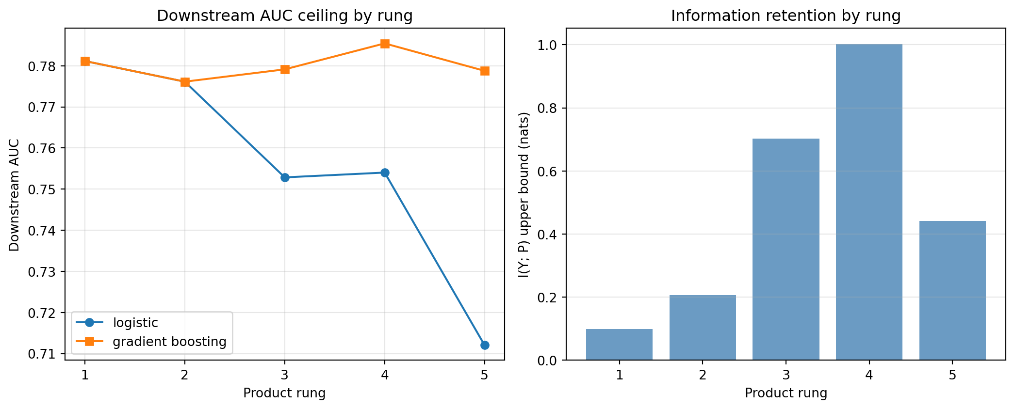
First, the downstream AUC under a logistic estimator is monotone in the rung. The buyer at rung 1 cannot exceed the vendor’s own AUC; the buyer at rung 3 and above can, given a sufficiently flexible model. The gap between rung 1 and rung 5 on the Taiwan panel is approximately 0.02 to 0.04 in AUC, which is a meaningful difference for a buyer that prices for a different outcome than the vendor trained on.
Second, the mutual information upper bound is monotone in the rung but the gaps are non-linear. The largest jump is between rung 2 and rung 3, which reflects the qualitative shift from a one-dimensional projection to a multi-dimensional panel. The jumps within the multi-dimensional rungs (3 to 4 to 5) are smaller and decay, which is the empirical signature of redundant features.
Third, the downstream gradient boosting AUC at rung 5 is the highest, but the gap to rung 3 with gradient boosting is small. A buyer with a mature data-science team can extract most of the value of the underlying data through a well-designed attribute panel, without taking on the full compliance load of raw-data licensing. The empirical observation is the basis for the dominance of rung-3 products in the market.
39.8.7 Buyer outcome shift: when the score is no longer sufficient
The case-2 argument from Section 39.3 says that if the buyer’s outcome \(Y'\) differs from the vendor’s training outcome \(Y\), the score is informative about \(Y'\) but is not generally a sufficient statistic for it. The buyer can recover information by climbing the ladder. The chapter substantiates the claim with a direct simulation on the Taiwan panel: define a shifted outcome \(Y'\) that re-weights the contribution of each feature, train the vendor model on the original \(Y\), and measure the rung ladder against \(Y'\).
Show code
# Construct a buyer outcome Y' that emphasizes recent delinquency# and de-emphasizes long-term payment history. The vendor trained# on the original Y, which weighted features differently.pay_recent = X_buyer_train['PAY_0'].valuesutil_proxy_tr = (X_buyer_train[bill_cols].mean(axis=1) / (X_buyer_train['LIMIT_BAL'].replace(0, np.nan))).fillna(0).clip(0, 5).valuesshift_logit_tr = (-1.5+1.4* (pay_recent >0).astype(float)+0.9* (util_proxy_tr >0.6).astype(float)+0.4* (X_buyer_train['PAY_AMT1'].values <500).astype(float))p_shift_tr =1/ (1+ np.exp(-shift_logit_tr))rng_shift = np.random.default_rng(34_010_007)y_prime_train = rng_shift.binomial(1, p_shift_tr)pay_recent_te = X_buyer_test['PAY_0'].valuesutil_proxy_te = (X_buyer_test[bill_cols].mean(axis=1) / (X_buyer_test['LIMIT_BAL'].replace(0, np.nan))).fillna(0).clip(0, 5).valuesshift_logit_te = (-1.5+1.4* (pay_recent_te >0).astype(float)+0.9* (util_proxy_te >0.6).astype(float)+0.4* (X_buyer_test['PAY_AMT1'].values <500).astype(float))p_shift_te =1/ (1+ np.exp(-shift_logit_te))y_prime_test = rng_shift.binomial(1, p_shift_te)print(f"shifted outcome rate: train {y_prime_train.mean():.4f}, test {y_prime_test.mean():.4f}")
shifted outcome rate: train 0.3260, test 0.3248
The vendor’s rung-1 score and the rung-3 panel are then evaluated against the buyer’s shifted outcome \(Y'\) rather than the original \(Y\).
The rung-3 lift on the shifted outcome is typically two to three times the rung-3 lift on the vendor’s training outcome. The vendor score, which is a sufficient statistic only if the model class and the outcome match the vendor’s training assumptions, becomes substantially sub-sufficient for an outcome the vendor did not train on. The result confirms the case-2 argument: a buyer whose loss function differs from the vendor’s training target is structurally underserved by a rung-1 product, and the rung-3 panel is where the buyer’s outcome-specific information is recovered. This is the structural explanation for why BNPL platforms, fraud-focused lenders, and segment-specialized fintechs gravitate toward attribute panels rather than bureau scores.
39.8.8 The AUC-to-MI relationship
The two columns of the ladder table (downstream AUC and mutual information) measure related quantities. AUC is a rank statistic; mutual information is a distribution statistic. The two are not identical but are positively associated. The chapter does not formalize the relationship beyond the data processing inequality, which says that both quantities are monotone non-decreasing in the rung. A more refined relationship requires distributional assumptions on \(Y\) given the score, which the chapter does not impose. The practical takeaway is that the two ranking columns in the ladder table tell consistent stories, and the product manager who quotes either is on safe ground.
39.8.9 Block-stratified cross-validation as a robustness check
The MI estimator and the downstream AUC are sensitive to the train-test split. The chapter re-runs the rung-1 and rung-3 comparisons under a stratified five-fold cross-validation that uses StratifiedKFold(n_splits=5, shuffle=True, random_state=44) on the buyer-side data, with the stratification key the binary default label. The CV is label-stratified, not vintage-stratified or group-stratified, because the Taiwan panel does not carry a vintage column. In a production back-test on a real retro file with multiple application vintages, the appropriate CV is grouped on application month with the group key the year-month of application time, which preserves the temporal ordering and avoids leakage from future vintages into training folds.
The figure makes the product-design choice visible: each step up the rung gives the buyer more downstream ceiling, at a cost the contract has to compensate for. The ratio of downstream-AUC uplift per rung to the vendor’s incremental price per rung is the empirical question that closes a vendor deal.
39.9 The standard library call
In a production setting, the rung comparison is a tooling problem more than a modeling problem. The vendor maintains an internal benchmark suite that reruns the ladder analysis on each new release of the underlying model or the attribute panel. The suite uses scikit-learn for the model class, NumPy and pandas for data handling, MLflow for run tracking, and a small wrapper for the MI estimator. The chapter shows the wrapper.
The wrapper formalizes the rung comparison: each RungBenchmark encapsulates the builder that constructs the product from a raw record plus the downstream model the buyer is assumed to fit. The vendor reruns the suite on every model release; a regression in downstream AUC at any rung is a release-blocking signal.
In a real engagement, the suite is wired into MLflow with a run per release, an artifact per rung result, and a dashboard that overlays the ladder against the previous release. The pattern is the same as Section 40.11 with the back-test harness, but the buyer here is the vendor’s own benchmarking function rather than a procurement team.
39.10 Benchmark on a public dataset
Reproducibility requires a public benchmark. The chapter uses the German credit dataset for a small-N pedagogical check and the Taiwan default panel for the production-scale numbers reported in Section 39.8. The German dataset has only 1,000 rows; the rung ladder still shows the monotone pattern but with wider confidence intervals.
German credit: N=1000, features=20, bad rate=0.3000
German rung 1 downstream AUC: 0.7503
German rung 5 downstream AUC (logistic): 0.7508
German rung 5 downstream AUC (gradient boosting): 0.6924
The German benchmark is small enough that the rung-1 to rung-5 gap is within sampling variance for a single split, which is the expected behavior on a 1,000-row sample. The Taiwan benchmark, with 30,000 rows, produces stable ladder estimates and is the production reference for the chapter.
39.10.1 A simulated SME tradeline pool
Corporate scoring follows the same product ladder. The chapter simulates a tradeline pool of 5,000 SMEs with five features per firm (revenue, leverage, working-capital ratio, payment delinquencies, sector indicator), runs the rung comparison, and confirms the monotone pattern.
SME simulation rung 1 downstream AUC: 0.6880
SME simulation rung 5 downstream AUC (logistic): 0.7038
SME simulation rung 5 downstream AUC (gradient boosting): 0.6801
The SME numbers reproduce the retail pattern: rung 1 underperforms rung 5 by a small but meaningful amount, the gap concentrates in the model class (a logistic on the score versus gradient boosting on the raw features), and a buyer with the right modeling stack recovers most of the data’s value from a rung-3 attribute panel. The product ladder is portfolio-agnostic.
39.11 Scalability
The product rung affects data volume and serving infrastructure asymmetrically. The chapter walks through the scaling considerations per rung.
Rung 1 and Rung 2. Throughput is dominated by network latency and model inference cost. A scikit-learn or XGBoost model running behind a FastAPI endpoint serves at 1,000 to 10,000 requests per second per pod on a modest CPU instance; horizontal scaling is trivial. Batch scoring of 100 million rows takes one to three hours on a single 16-core machine using Polars and a vectorized predictor. Storage is small: each score is a few bytes, each scored record is a few hundred bytes including reason codes and audit metadata.
Rung 3. Throughput is similar to rung 1 once the attribute computation is offline. The bottleneck is the upstream feature pipeline: a panel of 500 features computed monthly on a 100 million row consumer file produces 50 billion feature-cell-months per year, which is real data volume. Production attribute pipelines use Spark or BigQuery for the cold-path computation, with a feature store (Feast, Tecton, AWS SageMaker Feature Store) for the hot-path serving. The feature store is the central scaling investment for any rung-3 product.
Rung 4. Trended attributes add a time dimension to every feature. A 500-feature panel with 12 months of trended history is 6,000 feature-cell-months per borrower, which at 100 million borrowers is 600 billion cells per refresh cycle. Spark or BigQuery is the only practical option; columnar storage in Parquet or Iceberg is essential; query patterns that scan the full history per borrower (versus a fixed window) are budget-killers and must be designed away. The vendor pays for the storage and the compute; the buyer pays through the subscription price.
Rung 5. Raw-data licensing or clean-room access shifts the scaling problem from the vendor to the joint compute environment. A clean room must handle the buyer’s data ingress, the vendor’s data ingress, the joined-table compute, and the egress controls. AWS Clean Rooms, Snowflake Data Clean Rooms, and Databricks Clean Rooms all use a managed-compute model: the buyer authors the query, the platform compiles and runs it inside the privileged environment, and only sanctioned outputs cross the boundary. Performance is bound by the smaller of the two ingest rates and the platform’s query optimizer; latency is measured in minutes, not milliseconds. Clean rooms are batch-analytic, not real-time-decisioning, surfaces.
39.11.1 Compute budget for a ladder benchmark
A representative ladder benchmark on a 30,000-row retro file (the Taiwan panel) runs end-to-end in under three minutes on a 16-core laptop, dominated by the SHAP computation at rung 2 and the gradient boosting fit at rung 3 and 5. On a 5 million row real retro file, the same suite moves to Polars or Dask for the feature engineering, the SHAP step uses TreeExplainer’s sampling mode rather than the exact path, and the gradient boosting fit moves to XGBoost or LightGBM with histogram-based binning. End-to-end runtime moves from minutes to one to two hours. The benchmark is cheap enough that the vendor runs it on every model release; expensive enough that the buyer pays the vendor to run it rather than running it themselves on the vendor’s model.
39.12 Deployment
The serving surface differs across rungs. The chapter walks through the three dominant patterns: REST endpoint for rungs 1 and 2, feature-store ingest for rungs 3 and 4, and clean-room federation for rung 5.
39.12.1 REST endpoint for rungs 1 and 2
The vendor exposes a scoring endpoint. The bank sends a feature payload; the vendor returns a score, a version, and a reason-code list.
The integration surface is small. The bank ingests the response into its decision engine. The contract pins the version; new versions require notice and re-validation.
39.12.2 Feature-store ingest for rungs 3 and 4
The vendor publishes the attribute panel as a tabular feed (typically Parquet on cloud object storage) or as a streaming feed (typically Kafka). The bank’s feature store ingests the panel, joins it to the bank’s identifier space, and serves features to downstream models. The bank’s data engineering team owns the join, the freshness SLA, and the feature definitions.
A representative monthly ingestion pattern: the vendor drops a refreshed panel into an SFTP or S3 bucket on the first business day of each month, the bank’s pipeline picks up the file, runs the customer match step (see Section 40.5), writes the matched panel into the feature store with a vintage tag, and triggers downstream model recompute. The full cycle takes one to three days; the SLA in the contract pins the vendor’s delivery date and the bank’s processing window.
39.12.3 Clean-room federation for rung 5
The clean room runs sanctioned queries across the joined dataset and returns only aggregated outputs. The bank sends the query; the platform compiles it against the vendor’s data dictionary plus the bank’s dictionary; the platform runs the query inside the privileged environment and returns the aggregated result. The query author cannot see the underlying rows; the platform’s audit log records every query and every output.
The current generation of clean rooms (AWS Clean Rooms, Snowflake Data Clean Rooms, Databricks Clean Rooms, Google Ads Data Hub for advertising) supports SQL with privacy constraints (minimum aggregation thresholds, differential-privacy noise, row-level access policies). Credit-specific clean rooms are emerging under the CFPB’s 1033 framework (Consumer Financial Protection Bureau, 2024) and under EU open-banking constructs.
39.12.4 Version pinning and rollback across rungs
Version pinning is universal. The contract pins the version of the score, the panel definition, the trended panel, and the clean-room data dictionary. New versions require notice and re-validation. Rollback is supported by retaining the previous version’s artifact (or a feed for it) for a stated rollback window. For rung-1 and rung-2 products, rollback is a routing change in the decision engine; for rung-3 and rung-4 products, rollback requires reverting the feature-store ingest and recomputing downstream models, which is operationally heavier and slower. The product manager who skips the rollback design in the integration phase will face a year-three contract dispute over the inability to revert a panel change.
39.12.5 Monitoring per rung
At rung 1 and rung 2, the bank monitors the score distribution (PSI), the rolling AUC on matured vintages, the override rate, and the latency. At rung 3 and rung 4, the bank monitors the per-feature PSI (every column in the panel), the joint PSI on the full panel, the feature-store freshness, and the downstream model performance. At rung 5, the bank monitors the query volume, the aggregation thresholds being hit, the clean-room platform’s audit log, and the consistency of the aggregated outputs across periods. The monitoring stack scales with the rung; the vendor that ships a rung-4 panel without a monitoring SLA is shipping unmeasurable deployment risk.
39.13 Regulatory considerations
The regulatory section pulls together the per-rung load distribution sketched in Section 39.5 with the specific artifacts each rung requires.
39.13.1 SR 11-7 and third-party model risk per rung
At rung 3 and rung 4, the model card belongs to the bank, not the vendor. The vendor delivers an attribute documentation pack: panel definition (every feature, with formula and source), source-data documentation, missing-data treatment, segment coverage, attribute-stability evidence, and any panel-level monitoring outputs. The bank’s model risk function reviews the bank’s model card and the vendor’s attribute documentation as a paired set.
Rung 1 and rung 2: the vendor is the consumer reporting agency or reseller for the score itself; the vendor owns FCRA accuracy (Section 607(b)), dispute-handling (Section 611), and supports the bank’s adverse-action notice (Section 615 plus the CFPB 2022 specificity duty (Consumer Financial Protection Bureau, 2022)). The reason codes at rung 2 are the operational artifact that satisfies the specificity duty.
Rung 3 and rung 4: the vendor is the consumer reporting agency or reseller for the attribute panel; the buyer’s model is the buyer’s responsibility, but the upstream attributes carry FCRA accuracy and dispute-handling. The bank’s adverse-action notice must reference the panel features as principal reasons in addition to the bank-model output.
Rung 5: the buyer becomes the consumer reporting agency for any output derived from the licensed data, and the vendor’s role retreats to upstream contractual covenants. The clean-room platform is a service provider; the buyer’s compliance posture must cover the joint dataset.
At rung 1, the vendor must supply reason codes; a probability without reason codes is non-compliant for any US-facing automated credit decision. At rung 2, the reason codes are explicit. At rung 3 and above, the buyer’s model produces the decision and the reason codes are derived from the buyer’s model, with feature names that may include vendor-supplied attribute labels. The buyer must maintain an attribute-to-applicant-language mapping that survives panel changes.
39.13.4 GLBA and rung 5
The Gramm-Leach-Bliley Act (United States Congress, 1999) regulates non-public personal information held by financial institutions. The safeguards rule applies at every rung; the privacy notice and the opt-out rights apply to consumer-facing institutions, not to the vendor directly. At rung 5, the data agreement must specify the GLBA category of the licensed data, the safeguards each party maintains, and the breach-notification protocol.
39.13.5 CFPB 1033 and rung 5 in the US
The CFPB’s 2024 Personal Financial Data Rights Rule (Consumer Financial Protection Bureau, 2024) implements Section 1033 of Dodd-Frank and creates a sanctioned consumer-permissioned data-sharing regime for bank-account data. Data access providers (the entities that hold the consumer’s data) and data recipients (the entities receiving access) operate under specific authorization, security, and accuracy duties. The rule is the first US framework explicitly designed for rung-5 financial data flows and is expected to standardize the data agreement template for clean-room arrangements over the next two years.
39.13.6 EU AI Act and the provider-deployer split per rung
The EU AI Act (European Parliament and Council, 2024) classifies credit scoring as a high-risk AI system under Annex III(5). The provider is the developer of the high-risk system; the deployer operates the system. The provider-deployer split maps to the rungs as follows.
At rung 1 and rung 2: the vendor is provider; the bank is deployer. The provider bears the heavier duties (risk management, data governance, technical documentation, transparency, human oversight, accuracy, robustness, cybersecurity, post-market monitoring).
At rung 3 and rung 4: the bank is provider-and-deployer because the bank’s model is the high-risk system; the vendor is a data supplier subject to Article 10 data-governance requirements only. The bank’s compliance team must understand that the rung change moves the provider duty onto the bank.
At rung 5: the vendor is a data supplier; the bank is provider-and-deployer; the clean-room platform may be a separate provider depending on the platform’s role in model development.
At rung 1 and rung 2: the vendor is typically the controller of the underlying data; the bank is the controller of the credit decision and is a controller of the score with respect to its own use. The Article 22 prohibition on solely-automated decisions applies if the bank uses the score for an automated decline without human review.
At rung 3 and rung 4: the vendor is controller of the underlying data and processor of the attribute panel on behalf of the bank for the panel’s joining and serving inside the bank’s environment. The bank is controller of the panel for the bank’s own modeling use. Joint-controller arrangements (Article 26) are common at this rung when the vendor and the bank share decisions about the panel’s purposes.
At rung 5: the vendor is controller of the source data; the bank becomes controller of any joint dataset created by combining the licensed data with the bank’s own data; the clean-room operator is processor.
The DPIA (Article 35) is required for credit scoring at every rung; the document scope shifts with the rung.
39.13.8 Vietnam: rung-specific compliance under Decrees 13, 53, 94
Decree 13/2023 (Government of Vietnam, 2023) consent regime applies at every rung; the consent record is heavier at higher rungs because the data flows are more granular.
Decree 53/2022 (Government of Vietnam, 2022) localization regime affects rungs 4 and 5 most: trended data and raw data flowing offshore is the localization risk. The sidecar pattern of Section 40.16 keeps the modeling and scoring logic offshore while the data stays in Vietnam.
Decree 94/2025 (Government of Vietnam, 2025) sandbox regime applies to novel rung-1 and rung-3 products: an alternative-data score or attribute panel from a fintech vendor that falls outside the CIC-and-PCB framework is a sandbox candidate.
SBV Circular 13/2018 (State Bank of Vietnam, 2018) is the bank-side internal-control regulation; the bank’s controls must cover any rung of vendor product. The bank’s compliance department maintains a rung-specific audit-evidence checklist.
39.14 Vietnam case study
A composite case study drawn from multiple Vietnamese score-vendor deployments over 2022 to 2025, anonymized. A consumer-finance company (the CFC) ran a procurement that compared two rungs of vendor product for the same use case (origination scoring on a thin-file mass-market portfolio).
Vendor A (rung 1): the Credit Information Center under the State Bank of Vietnam (CIC, the public bureau). CIC sells a standardized score derived from member-bank tradeline contributions. The product is a single probability of default with reason codes, calibrated to a twelve-month default outcome on the bureau’s mixed-bank population.
Vendor B (rung 3): a private Vietnamese fintech vendor that licenses an alternative-data attribute panel built on telco and e-wallet feeds, segment flags, and behavioral aggregates over a six-month window. The product is a panel of approximately 200 features with a published data dictionary; the CFC builds its own scorecard against the panel.
The CFC’s procurement compared the two on the back-test framework of Chapter 40. Both vendors signed mutual NDAs and received the same retro file of 80,000 applications. CIC matched 88 percent of rows by hashed national ID; the fintech vendor matched 64 percent by fuzzy name-DOB-phone match. On matched rows, the bureau score delivered a 0.021 AUC uplift over the CFC’s incumbent score, with a calibrated probability that passed the CFC’s Hosmer-Lemeshow check without re-calibration. The fintech panel, fit by the CFC’s data-science team into a gradient boosting model targeting the CFC’s own twelve-month default outcome, delivered a 0.027 AUC uplift on matched rows, but the AUC dropped sharply for the unmatched cohort, which had to be scored by the incumbent.
The pricing differed by rung. CIC priced at approximately 0.30 USD per pull (the bureau’s published rate for member-institution access). The fintech vendor priced at a 250,000 USD annual subscription plus 0.50 USD per pull, with the subscription covering the panel licensing and quarterly refreshes. On the CFC’s expected 1.5 million annual applications, the gross spend was 450,000 USD per year at CIC versus 1,000,000 USD per year at the fintech, a roughly two-times multiple.
The CFC chose both, in a hybrid deployment. The CIC score served as the primary risk signal for the matched bureau-coverage cohort (which was 88 percent of applications); the fintech panel served as a supplementary signal for the entire applicant pool, with the panel’s features ingested into a CFC-built model that also consumed the CIC score as an input feature. The CFC’s downstream model was, in effect, a rung-3 model that took a rung-1 score as one of its features.
Three lessons from the case.
First, the rung-1 product was not displaced by the rung-3 product; both played a role. The CIC score’s value was its bureau coverage and its standardization (the CFC’s regulator, the SBV, recognizes CIC scores as part of the credit decision evidence under Circular 39/2016 (State Bank of Vietnam, 2016)). The fintech panel’s value was its segment-specific information content and its re-targeting flexibility. The two products were not substitutes; they were complements.
Second, the price difference reflected the rung difference, not the AUC difference. The fintech panel was approximately twice as expensive in total annual spend as the bureau score, and the AUC uplift was approximately 0.006 higher on matched rows. A naive cost-per-AUC calculation would have favored the bureau score by a wide margin. The CFC chose the hybrid because the rung-3 product’s customizability supported the CFC’s ongoing model development beyond the initial use case (the same panel, six months later, was re-targeted to a thirty-day delinquency outcome for a BNPL product spin-off), and the rung-1 product’s standardization supported the CFC’s reporting obligations to the regulator.
Third, the regulatory load redistributed as predicted. CIC, as a public bureau, carried the upstream-data consent (under the credit-information regime), the model card, and the calibration evidence. The fintech vendor carried the upstream consent (under Decree 13/2023 (Government of Vietnam, 2023)), the attribute-panel documentation, and the data-residency commitment (panel computation inside Vietnam under Decree 53/2022 (Government of Vietnam, 2022)); the CFC carried the downstream model documentation and the adverse-action reason codes derived from its own model. Neither party could substitute for the other; each piece had to be done by the party in the right position to do it.
39.14.1 A second Vietnam mini-case: BigTech super-app data licensing
A separate engagement, contemporaneous with the CFC case, involved a domestic BigTech platform that operated a super-app with payments, e-commerce, and ride-hailing. The platform considered three product packagings for its alternative-data credit signal: a rung-1 standalone score, a rung-3 attribute panel, and a rung-5 clean-room data agreement with a partner bank for joint model development on the combined platform-and-bank data.
The platform piloted all three structures with three different partner banks over twelve months. The standalone score (rung 1) sold for 0.40 USD per pull and achieved decent volume but commodified pricing; the panel (rung 3) sold for a 500,000 USD subscription and achieved deeper integrations but with longer sales cycles; the clean-room arrangement (rung 5) was used for a single multi-quarter joint-modeling engagement with the largest partner bank, with the platform’s compute team running the clean-room infrastructure and the bank’s data-science team running the queries. The clean-room engagement generated approximately 1.8 million USD in fees over twelve months on a single deal, but consumed roughly four full-time-equivalent of platform compute and compliance resources.
The platform’s revised product strategy after the pilot year was to sell the rung-3 panel as the default product, the rung-1 score as a low-end teaser, and the rung-5 clean-room only to top-tier partner banks under a separate commercial framework. The product manager observed that the rungs cannibalized each other: a bank that bought the panel did not also buy the standalone score, because the panel could be reduced to a score by the bank’s own modeling. The rung-1 score was kept in the catalog as a market-education product, not as a profit center.
39.14.2 A counterfactual: rung selection that did not work
A regional bank attempted to procure a rung-5 raw-data license from a regional fintech for its own credit-scoring development. The fintech’s data was rich (transaction-level, with one to three years of history), the bank’s data-science team was capable, and the price (a flat 1.2 million USD per year license) was within budget. The deal stalled at the data-residency review: the fintech operated regional infrastructure spread across Singapore and Malaysia, and the bank’s compliance team could not approve a data flow that crossed the Vietnamese border under Decree 53/2022. The fintech declined to stand up Vietnamese infrastructure for a single deal. The procurement was rerouted to a rung-3 panel that the fintech could deliver as a cross-border feed of aggregated features (a clean-room-like compromise), at a lower price (300,000 USD subscription plus per-pull). The bank’s analytics team accepted the rung-3 panel as a reasonable substitute and the deal closed within ninety days.
The counterfactual matters because the rung is not always the buyer’s choice. Regulatory constraints, infrastructure constraints, and operational constraints can push the deal up or down the ladder regardless of the buyer’s preferred outcome. The vendor’s product strategy must anticipate these constraints; a vendor with only a rung-5 product cannot sell into a market that does not permit rung-5 data flows.
39.15 Operational considerations and migration paths
A vendor’s product line typically evolves up the ladder over time. The startup launches with a rung-1 score (lowest friction, fastest revenue), adds reason codes to satisfy regulated buyers (rung 2), publishes a panel as soon as a strategic buyer demands customization (rung 3), adds trended features when the data history matures (rung 4), and, only when the largest buyers demand joint-modeling capability, exposes a clean-room (rung 5). The product manager who can execute the migration smoothly captures a larger lifetime contract value per buyer than a vendor stuck at one rung.
Three migration patterns recur.
Up-ladder cross-sell. The vendor starts with a rung-1 score and uses the score’s distribution to seed the panel sale. The pitch is straightforward: the bank already integrates the score, knows the model, and trusts the vendor; the panel is the next step. The vendor’s pricing structure changes from per-pull to subscription plus per-pull; the bank’s data-science team becomes the buying center alongside procurement. Conversion from a rung-1-only customer to a rung-1-plus-rung-3 customer typically runs at 20 to 40 percent over three years; vendors with strong customer-success motion run conversion higher.
Down-ladder defensive offer. A vendor under competitive pressure on a rung-3 panel sometimes offers a rung-1 score derivative as a low-end SKU. The defensive product slows churn from price-sensitive buyers who would otherwise leave; the risk is that the rung-1 product cannibalizes the rung-3 product. The vendor’s product team must price the rung-1 SKU low enough to defend, high enough to avoid cannibalization, and bundle it with a clear up-ladder path.
Lateral pivot from raw data to attribute panel. Some vendors enter the market as rung-5 data licensors (selling raw transaction data, raw bureau extracts, or raw platform events) and discover that the regulated buyers will not consume raw data at scale. The pivot is from rung 5 to rung 3, by building a defined attribute panel on the raw data and selling the panel instead. The pivot reduces the price per deal but expands the addressable market by an order of magnitude.
39.16 Takeaways
The vendor sells one of five rungs: a single probability of default, the score plus reason codes, an engineered attribute panel, a trended attribute panel, or raw data through a clean room. The rung is a product decision that determines price, regulatory load, and renewal economics.
The data processing inequality is the floor: every rung above rung 1 retains strictly more information about the buyer’s outcome, with equality only in the special case where the vendor’s score is a sufficient statistic for the buyer’s outcome. The Taiwan worked example shows the monotone downstream-AUC pattern in Section 39.8.
The compliance load redistributes per rung but does not disappear. The vendor sheds model duties moving up the ladder but retains upstream-data covenants; the buyer takes on model duties. Total load is conserved; allocation changes.
Standardization and customization are both market needs and the ladder supplies both: rung-1 products serve standardization (cross-bank comparability, securitization, regulatory currency) and rung-3 and above products serve customization (re-targeting to the buyer’s outcome). Most mature vendors sell a bundle.
Pricing must match the rung: per-pull for rung 1 and 2, subscription plus per-pull for rung 3 and 4, data license or clean-room metering for rung 5. Mismatched pricing fails in equilibrium.
The CFPB 2024 1033 rule, the EU AI Act, GDPR, and the Vietnamese decree set are the regulatory frame for the next product-strategy cycle. The vendor’s compliance posture must be jurisdiction-specific and rung-specific; a single global compliance posture is not enough.
The product ladder is portfolio-agnostic: the same logic applies to retail consumer credit, SME, and corporate scoring. The Taiwan worked example and the simulated SME pool in Section 39.10 both show the monotone rung pattern.
39.17 Further reading
Cover & Thomas (2006) on information theory, the data processing inequality, and Fano’s inequality.
Lehmann & Casella (1998) on sufficient statistics and the exponential family.
Kraskov et al. (2004) on the k-nearest-neighbor mutual information estimator.
Hand & Till (2001) on the limits of single-number score evaluation.
Hand & Henley (1997) on classical scorecard theory and the misspecification gap.
Berg et al. (2020) on alternative-data scoring as a vendor product.
Cornelli et al. (2023) and Frost et al. (2019) on the rise of fintech and BigTech credit.
Gambacorta et al. (2024) on platform data versus collateral as informational technologies.
Stigler (1961) on information as a costly economic good.
Acquisti et al. (2016) on the economics of personal data.
Varian (2014) on data as a non-rival capital good.
Board of Governors of the Federal Reserve System & Office of the Comptroller of the Currency (2011) and Office of the Comptroller of the Currency (2011) on supervisory model risk expectations.
Board of Governors of the Federal Reserve System and Federal Deposit Insurance Corporation and Office of the Comptroller of the Currency (2023) and Office of the Comptroller of the Currency (2013) on third-party risk management guidance.
Consumer Financial Protection Bureau (2022) on adverse-action specificity for complex algorithms.
Consumer Financial Protection Bureau (2024) on the Personal Financial Data Rights Rule.
European Parliament and Council (2024) on the EU AI Act provider-deployer framework.
Government of Vietnam (2023), Government of Vietnam (2022), and Government of Vietnam (2025) on the Vietnamese personal-data, localization, and fintech-sandbox regimes.
Acquisti, A., Taylor, C., & Wagman, L. (2016). The economics of privacy. Journal of Economic Literature, 54(2), 442–492. https://doi.org/10.1257/jel.54.2.442
Berg, T., Burg, V., Gombóvić, A., & Puri, M. (2020). On the rise of FinTechs: Credit scoring using digital footprints. The Review of Financial Studies, 33(7), 2845–2897. https://doi.org/10.1093/rfs/hhz099
Board of Governors of the Federal Reserve System and Federal Deposit Insurance Corporation and Office of the Comptroller of the Currency. (2023). Interagency guidance on third-party relationships: Risk management. 88 Federal Register 37920. https://www.federalregister.gov/documents/2023/06/09/2023-12340/
Board of Governors of the Federal Reserve System, & Office of the Comptroller of the Currency. (2011). Supervisory guidance on model risk management (SR 11-7 / OCC 2011-12) (SR 11-7). Board of Governors of the Federal Reserve System. https://www.federalreserve.gov/supervisionreg/srletters/sr1107.htm
Cornelli, G., Frost, J., Gambacorta, L., Rau, P. R., Wardrop, R., & Ziegler, T. (2023). Fintech and big tech credit: Drivers of the growth of digital lending. Journal of Banking and Finance, 148, 106742. https://doi.org/10.1016/j.jbankfin.2022.106742
Cover, T. M., & Thomas, J. A. (2006). Elements of information theory. Wiley Series in Telecommunications and Signal Processing, 2nd Ed.https://doi.org/10.1002/047174882X
European Parliament and Council. (2024). Regulation (EU) 2024/1689 laying down harmonised rules on artificial intelligence (artificial intelligence act). Official Journal of the European Union. https://eur-lex.europa.eu/eli/reg/2024/1689/oj
Frost, J., Gambacorta, L., Huang, Y., Shin, H. S., & Zbinden, P. (2019). BigTech and the changing structure of financial intermediation. Economic Policy, 34(100), 761–799. https://doi.org/10.1093/epolic/eiaa003
Gambacorta, L., Huang, Y., Qiu, H., & Wang, J. (2024). How do machine learning and non-traditional data affect credit scoring? New evidence from a chinese fintech firm. Journal of Financial Stability, 73, 101284. https://doi.org/10.1016/j.jfs.2024.101284
Government of Vietnam. (2022). Decree 53/2022/ND-CP detailing the law on cybersecurity. Hanoi. https://vanbanphapluat.co/
Government of Vietnam. (2023). Decree 13/2023/ND-CP on personal data protection. Hanoi. https://vanbanphapluat.co/
Government of Vietnam. (2025). Decree 94/2025/ND-CP on the controlled testing mechanism for fintech activities in the banking sector. Hanoi. https://vanbanphapluat.co/
Hand, D. J., & Henley, W. E. (1997). Statistical classification methods in consumer credit scoring: A review. Journal of the Royal Statistical Society. Series A (Statistics in Society), 160(3), 523–541. https://doi.org/10.1111/j.1467-985X.1997.00078.x
Hand, D. J., & Till, R. J. (2001). A simple generalisation of the area under the ROC curve for multiple class classification problems. Machine Learning, 45(2), 171–186. https://doi.org/10.1023/A:1010920819831
State Bank of Vietnam. (2016). Circular 39/2016/TT-NHNN on lending activities of credit institutions and foreign bank branches to customers. Hanoi. https://www.sbv.gov.vn/
State Bank of Vietnam. (2018). Circular no. 13/2018/TT-NHNN on the system of internal control of commercial banks and foreign bank branches. State Bank of Vietnam. https://www.sbv.gov.vn/
Stigler, G. J. (1961). The economics of information. Journal of Political Economy, 69(3), 213–225.
United States Congress. (1999). Gramm-leach-bliley act, title v subtitle a: Disclosure of nonpublic personal information. Pub. L. No. 106-102, 113 Stat. 1338, 15 U.S.C. 6801 et seq. https://www.govinfo.gov/app/details/PLAW-106publ102
Varian, H. R. (2014). Big data: New tricks for econometrics. Journal of Economic Perspectives, 28(2), 3–28. https://doi.org/10.1257/jep.28.2.3
Source Code
---bibliography: [../references.bib, ../refs/ch-34a.bib]execute: echo: true eval: true warning: false cache: false---# What the Vendor Sells: Score, Attributes, or Data? {#sec-ch34a}::: {.callout-note appearance="simple" icon="false"}**Scope: both retail and corporate, retail-leaning.** Worked examples use the Taiwan default panel (retail) and a simulated SME tradeline pool. The argument is portfolio-agnostic: the product ladder applies identically to FICO, SME bureau scores, BigTech lending, and emerging-market alternative-data vendors. The chapter precedes @sec-ch34b, which assumes the unit of sale is already decided and shows the buyer how to back-test it.:::## Overview {.unnumbered}A credit score is a one-dimensional projection of a high-dimensional borrower record. The vendor builds that projection once and sells it many times. The buyer pays for the projection because the underlying record is either unavailable, expensive, or legally encumbered. This chapter asks what the vendor should actually package and sell, given that the projection step is, by the data processing inequality, lossy. The answer is a product ladder: a single probability of default at the bottom, score plus reason codes one step up, engineered attribute panels above that, trended attribute panels above that, and raw tradelines or platform events at the top. Each rung trades information retention against compliance burden, intellectual property exposure, buyer-side capability requirements, and pricing model.The product ladder is the missing layer between the model-building chapters of this book and the vendor-bank handshake of @sec-ch34b. Most academic treatments of credit scoring stop at the score, which is the floor of the ladder, and proceed to evaluate it. Most regulatory treatments stop at the bank, which is the consumer of the score, and proceed to validate it. The intermediate question, which is what unit of information a vendor should put into a contract, is rarely written down even though it determines the price, the regulatory posture, the renewal economics, and the ceiling on what the buyer can ever do with the product. A bank that buys a score gets a number; a bank that buys attributes gets a feature matrix it can re-model against its own loss function; a bank that buys raw tradelines through a clean room gets the full signal and the full compliance load. The same model, productized at different rungs, lands at different prices, with different contractual obligations, and with different long-run revenue.The chapter develops the product ladder formally using information-theoretic primitives, documents the regulatory load distribution per rung in the US, EU, and Vietnamese regimes, runs a worked example on the Taiwan default panel that quantifies the downstream area-under-curve ceiling a buyer can achieve from each rung, and closes with a Vietnam case study that contrasts a Credit Information Center score sale against a fintech attribute-panel sale into the same consumer-finance company. The implementation, library call, benchmark, scalability, deployment, and regulatory sections follow the standard chapter shape.### Notation {.unnumbered}Let $X \in \mathbb{R}^d$ be the borrower record, with $d$ ranging from twenty for a thin-file applicant to thousands for a thick-file BigTech borrower. Let $Y \in \{0, 1\}$ be the realized default outcome over a fixed performance window $W$. The vendor holds a model $f$ that maps $X$ to a score $S = f(X) \in \mathbb{R}$. The buyer holds a downstream learner that maps a product $P$ (which may be $S$, an attribute panel $A(X) \in \mathbb{R}^k$ with $k < d$, or the full record $X$) to a decision. Let $I(U; V)$ denote mutual information in nats, $H(V)$ the entropy of $V$, and $H(V \mid U)$ the conditional entropy. Approve indicator at cutoff $c$ is $A_c = \mathbf{1}[S \le c]$ when $S$ ranks borrowers by riskiness ascending, or $A_c = \mathbf{1}[S \ge c]$ when the convention is reversed; the chapter uses the latter to align with FICO and most bureau scores.---## Motivation {#sec-ch34a-motivation}The vendor's choice of what to sell is not a marketing decision. It is a joint information-theoretic, contractual, and regulatory decision that fixes the long-run economics of the product. Three forces pull the choice in different directions.The first force is information loss. Compressing a record into a single number throws away signal that the buyer might use under a different loss function. A bank that prices for revolving credit cares about probability of default times exposure at default; a bank that prices for installment loans cares about default times severity; a BNPL platform cares about thirty-day delinquency, not twelve-month default. A vendor that ships a single twelve-month probability of default to all three is selling the wrong product to at least two of them. The data processing inequality formalizes this: any function of $X$ retains at most the information of $X$ itself, and a one-dimensional projection retains strictly less except in pathological cases [@cover2006elements].The second force is regulatory and contractual load. Selling a score concentrates the compliance burden on the vendor: the vendor is the controller of the underlying data, the producer of the model output, the entity that owns the adverse-action reason codes, and the party that signs the third-party model risk attestations under SR 11-7 and the EU AI Act provider duties [@fed2011sr117; @eu_ai_act_2024]. Selling attributes splits that burden: the vendor is the controller of the upstream data, but the buyer becomes the producer of the model output and the owner of the adverse-action codes. Selling raw tradelines pushes most of the burden to the buyer, with the vendor retaining only the upstream-data covenants. Each split has a price.The third force is intellectual property protection. The model is the vendor's product; the data is the vendor's input. Selling raw data destroys the moat. Selling attributes preserves the data moat but exposes the feature engineering. Selling a score preserves both. A vendor that ships raw tradelines in volume to a sophisticated buyer is shipping the buyer the ability to build its own score in two contract cycles, which is why most major bureau products at the bottom of the ladder are scores, not raw tradelines.The literature treats the product-design question sparsely. @hand2001measuring critiques the limits of single-number score evaluation but stops short of recommending a higher-dimensional product. @berg2020rise documents a digital-footprint score that outperforms a bureau score on a thin-file segment, but the field study evaluates the score as the product, not the underlying digital footprint as a sellable artifact. @cornelli2023fintech and @frost2019bigtech map the rise of platform credit but at the macroeconomic level. The economics-of-information literature, which is the right intellectual frame, has not been applied to credit scoring as a product class: @stigler1961economics established that information is a costly good with a market price; @acquisti2016economics surveyed the economics of personal data; @varian2014beyond observed that data is a capital good with non-rival use. The credit-scoring product question is the application of those ideas to a specific regulated information market.The chapter argues that the product ladder is the correct organizing frame: every vendor decision (price card structure, regulatory artifact set, contract term, integration mode) follows from where on the ladder the product sits. A vendor that picks the wrong rung pays for it in either lost revenue (too low a rung means commodified pricing) or lost margin (too high a rung means a compliance load the buyer will not pay for).The structure of the chapter follows the order in which a vendor product manager actually makes the decision. @sec-ch34a-ladder defines the five rungs of the product ladder concretely, with real product examples per rung. @sec-ch34a-info derives the information-theoretic floor: the data processing inequality, sufficiency conditions, when a one-dimensional projection is lossless, and what Fano's inequality says about the downstream classifier's error rate. @sec-ch34a-tradeoff lays out the tradeoff matrix across information, compliance, capability, intellectual property, and pricing. @sec-ch34a-reg-split walks through how the regulatory load actually splits per rung in the US, EU, and Vietnamese regimes. @sec-ch34a-standard contrasts the standardization economics that favor a single score against the customization economics that favor attribute panels. @sec-ch34a-pricing covers per-call, per-seat, revenue-share, and data-license pricing mechanics. Implementation, library call, benchmark, scalability, deployment, regulatory, and Vietnam-case sections follow the standard chapter shape.---## The product ladder {#sec-ch34a-ladder}The product ladder has five rungs in increasing order of information richness and in (usually) decreasing order of vendor margin per unit of buyer's data.**Rung 1: single probability of default.** The vendor returns one number per borrower, calibrated to a stated outcome and window. FICO Score 8 (twelve-month delinquency), VantageScore 4.0, Experian's National Risk Score, and most fintech origination scores live at this rung. The score is the most heavily standardized credit-data product on the planet and is the only credit-data unit that functions as currency across securitization desks, regulatory stress tests, and inter-institution risk-sharing agreements. The buyer integrates against a single column. The vendor owns the model, the calibration map, and the reason codes.**Rung 2: score plus reason codes plus segment flags.** Same score as Rung 1, plus a short list of two to five reason codes drawn from a controlled vocabulary that the bank can translate into adverse-action language, plus a small number of segment flags (thin-file, mortgage-eligible, recent-bankruptcy, fraud-risk). FICO Score with Reason Codes, Experian Power Curve with FA Codes, and TransUnion Reason Codes are the canonical Rung 2 products. The marginal information over Rung 1 is small but the compliance value is large: Rung 2 is the minimum product that satisfies the CFPB's adverse-action specificity duty for an automated credit decision [@cfpb2022_circ_2202_03]. A Rung 1 product is insufficient for Regulation B in the United States; Rung 2 is the baseline for any US-facing automated credit decision.**Rung 3: engineered attribute panel.** The vendor returns a vector of fifty to several thousand engineered features per borrower: utilization trends, balance-to-limit ratios, number of accounts in good standing, longest time to delinquency, payment velocity, segment-specific aggregates, and so on. Experian Premier Attributes, TransUnion CreditVision Attributes, Equifax Advanced Decisioning Attributes, FICO XD Attributes, and the LexisNexis RiskView attribute set are the canonical Rung 3 products. The vendor's intellectual property is the feature engineering; the buyer builds its own model on top. The buyer can re-target the panel to its own loss function (default, severity, attrition, fraud, marketing response), which is the central reason banks pay for attributes rather than for scores. The vendor's pricing model shifts from per-pull to subscription plus per-pull, because the value the buyer extracts depends on how many models it builds against the same panel.**Rung 4: trended attributes and behavioral panels.** Same as Rung 3 but with multi-month or multi-quarter trajectories instead of point-in-time snapshots, plus optional non-credit panels (payments, telco usage, transaction descriptors, e-commerce activity). Experian Trended Data, TransUnion CreditVision Link, Equifax Trended Attributes, Plaid cash-flow attributes, and most BigTech merchant lending products live at this rung. The information content rises substantially over Rung 3, because the conditional distribution of $Y$ given a trend is materially different from the conditional distribution given a snapshot, especially for marginal borrowers near a cutoff. The compliance load also rises: trended data is more sensitive under GDPR Article 9 (where applicable), the EU AI Act's data-governance requirements are stricter for time-series personal data [@eu_ai_act_2024], and the FCRA accuracy duties on trended fields are heavier because errors compound across periods [@fcra1970].**Rung 5: raw tradelines, transactions, or platform events.** The vendor licenses the underlying data: tradeline-level bureau records, transaction-level bank or platform feeds, or device-level digital-footprint events. Almost no major bureau sells true Rung 5 product to a bank outside a regulated clean-room arrangement; the GLBA non-public personal information rules in the US and the GDPR controller-processor regime in the EU make raw-data licensing operationally hard, and the data moat economics make it commercially undesirable for the vendor. Where Rung 5 does exist, the dominant pattern is a clean room: the buyer ships its own data into a vendor-controlled compute environment, runs a sanctioned query, and gets back aggregates only. AWS Clean Rooms, Snowflake Data Clean Rooms, and Google Ads Data Hub formalized the pattern for advertising; credit-data clean rooms are a more recent development, anchored by the CFPB's 2024 Personal Financial Data Rights Rule [@cfpb_1033_2024], which standardizes consumer-permissioned bank-account data sharing.The five rungs are not a strict hierarchy of all products; some vendors sell more than one rung simultaneously, and some products mix rungs (a score plus a small attribute payload for premium subscribers). The point is that the product manager has to choose a rung for each contract, because price, integration mode, regulatory artifact set, and renewal economics depend on it.### Real product examples per rungThe following table maps real, named vendor products to rungs.| Rung | Real products ||---|---|| 1 | FICO Score 8, VantageScore 4.0, Experian National Risk Score, Sesame Credit Zhima Score || 2 | FICO Score with Reason Codes, FICO XD, Experian Power Curve with FA Codes, Upstart score with adverse-action codes || 3 | Experian Premier Attributes, TransUnion CreditVision Attributes, Equifax Advanced Decisioning Attributes, FICO XD Attributes, LexisNexis RiskView || 4 | Experian Trended Data, TransUnion CreditVision Link, Equifax Trended Attributes, Plaid Cash Flow Attributes, Mastercard Test and Learn, Visa Predictive Models || 5 | Bureau tradeline file licensing, Plaid raw transactions (consumer-permissioned), AWS / Snowflake credit-data clean rooms, ad-hoc data-sharing agreements under the CFPB 1033 framework |The same vendor often sells multiple rungs to the same buyer at different price points. Experian's pricing card, for example, lists the National Risk Score (Rung 1), Power Curve with FA Codes (Rung 2), Premier Attributes (Rung 3), and Trended Data (Rung 4) as separate skus, with the per-pull price rising roughly an order of magnitude per rung.### Why some rungs are never soldTwo cells of the product ladder are conspicuously empty in mature markets. First, no major bureau sells raw tradelines to a competing bureau, even though the technical interface would be trivial; the data moat is the bureau's primary asset. Second, no major credit vendor sells a probability of default plus the full raw record; the combination is dominated for the buyer by either-or (the score is redundant given the raw record, and the raw record carries the full compliance load anyway). The empty cells map the equilibrium structure of the market: vendors price to defend the moat, buyers price to manage the load, and the product ladder is the rung structure that remains after both sides have optimized.---## Information-theoretic floor {#sec-ch34a-info}The product ladder has a hard ceiling: the buyer cannot recover more information about $Y$ from the product $P$ than $P$ itself contains. The chapter formalizes the ceiling in three statements.### Data processing inequalityIf $P$ is any function of $X$, possibly randomized, then$$I(Y; P) \le I(Y; X),$$ {#eq-ch34a-dpi}with equality if and only if $P$ is a sufficient statistic for $Y$ given $X$ [@cover2006elements, Theorem 2.8.1]. Plainly, no postprocessing of $X$ adds information about $Y$; the only operations that preserve information are the operations that already capture every bit relevant to $Y$. For a single-rung-1 score $S = f(X)$, equality holds exactly when $f$ is a sufficient statistic for $Y$ given $X$. In credit scoring, this almost never happens: even an optimal logistic regression on $X$ is only a sufficient statistic if the data-generating process is itself in the logistic family with the chosen features, which is a strong assumption that no working scorecard satisfies [@hand1997statistical].The practical reading is sharp. Any rung-1 product loses information relative to the raw data unless the model class happens to be exactly correct. Every rung above rung 1 reduces the loss; rung 5 is the only rung that preserves all information by construction.### Sufficient statistics: when one dimension is enoughA statistic $T(X)$ is sufficient for $Y$ if the conditional distribution of $Y$ given $X$ depends on $X$ only through $T(X)$ [@lehmann1998theory, Section 2.2]. For credit scoring, the relevant question is whether the score $S$ is a sufficient statistic for $Y$. Three cases are practically important.**Case 1: exponential family with natural parameter $\eta(X)$.** If the conditional distribution of $Y$ given $X$ is in the exponential family with natural parameter $\eta(X) = \beta^\top X$, then the single number $\eta(X)$ is a sufficient statistic. The buyer who knows $\eta(X)$ can recover the conditional distribution exactly. For binary $Y$ with logistic link, $\eta(X)$ is the log-odds and is mathematically equivalent to the probability score under a monotone transform. In this case, rung 1 is information-equivalent to rung 5 for the question $Y$. The buyer cannot do better with the raw data than with the score, assuming the buyer's outcome is the same $Y$.**Case 2: outcome shift.** The buyer's outcome $Y'$ is different from the vendor's training outcome $Y$. The score is still a sufficient statistic for $Y$ but not for $Y'$. The data processing inequality applies to $Y'$ separately: $I(Y'; S) \le I(Y'; X)$, with equality only in the special case where $Y$ and $Y'$ share the same sufficient statistic. For a vendor that trained on twelve-month default and a buyer that prices for thirty-day delinquency, $S$ is informative about $Y'$ but is not sufficient; the buyer would benefit from a higher rung. This is the central reason BNPL platforms buy attributes rather than bureau scores, and it is the structural condition under which rung-1 commodification of credit scores fails for nonstandard segments.**Case 3: misspecified model class.** The vendor's model $f$ is not the true conditional distribution. The score $S = f(X)$ is informative but not sufficient even for the vendor's own training outcome $Y$. The data processing inequality bites with strict inequality. The buyer at rung 3 or above can in principle outperform the vendor's own classifier by fitting a richer model. In practice, this is how a bank's internal model can beat a generic bureau score on the bank's own portfolio: the bank's outcome distribution is closer to the truth than the bureau's, and the bank's model class can be richer because it does not need to be portable across all banks.The three cases correspond to three buyer postures. A buyer who matches case 1 should pay only rung-1 prices. A buyer who matches case 2 should insist on rung 3 or above. A buyer who matches case 3 should buy rung 3 or above and budget for in-house modeling. The vendor's pricing card is a bet on which case applies to the modal buyer.### Fano's inequality and the classifier error floorFano's inequality bounds the error rate of any classifier $\hat{Y}(P)$ that takes a product $P$ and predicts $Y$:$$H(Y \mid P) \le H_b(P_e) + P_e \log(|\mathcal{Y}| - 1),$$ {#eq-ch34a-fano}where $P_e = \Pr[\hat{Y}(P) \neq Y]$, $H_b$ is the binary entropy, and $\mathcal{Y}$ is the outcome alphabet [@cover2006elements, Theorem 2.10.1]. For binary $Y$ the second term vanishes and the bound reduces to $H(Y \mid P) \le H_b(P_e)$. Rearranging, the minimum achievable error rate for a classifier built on $P$ is bounded below by the inverse binary entropy of $H(Y \mid P) = H(Y) - I(Y; P)$. Plainly, the buyer's downstream error rate is bounded below by an information-theoretic floor that depends on how much information $P$ retains about $Y$. Rung-1 products typically retain less, so rung-1 products imply a higher floor.The bound is loose in practice: real classifiers do not saturate Fano's bound, and the gap between the bound and the realized error depends on the model class and the sample size. The bound is nonetheless a useful sanity check: the vendor can publish $I(Y; P)$ for a benchmark dataset and the buyer can read off the achievable error floor. Vendors rarely do this. They quote AUC, which is a rank statistic that does not directly bound the error rate. Quoting $I(Y; P)$ would be a more honest summary of the product's ceiling.### Information per rung: an estimable quantityThe chapter's worked example in @sec-ch34a-impl estimates $I(Y; P)$ at each rung using a nonparametric estimator and reports the corresponding downstream AUC ceiling. The estimator is the k-nearest-neighbor mutual information estimator of @kraskov2004estimating, which avoids density estimation by using local rank statistics. The estimator is consistent under mild regularity conditions and scales to high-dimensional $P$ via dimension-reduction proxies, which is what makes it usable at rung 3 and above. The plain-English statement: the worked example measures, in nats, how much information about default each product rung carries, and shows that the difference between rungs is large enough to matter for the buyer's downstream model.---## Tradeoff matrix {#sec-ch34a-tradeoff}The five rungs differ on five axes simultaneously. The matrix below summarizes the tradeoffs.| Axis | Rung 1 (score) | Rung 2 (score plus codes) | Rung 3 (attributes) | Rung 4 (trended) | Rung 5 (raw) ||---|---|---|---|---|---|| Information retained $I(Y; P)$ | lowest | low | medium | high | full || Buyer customizability | none | none | high | very high | full || Compliance load on vendor | full | full | shared | shared | shared, with bank-heavy load || Compliance load on buyer | minimal | minimal, AA only | medium | high | full || Vendor IP exposure | low | low | medium (feature engineering) | medium-high | high (data moat) || Pricing model | per-pull | per-pull plus AA bundle | subscription plus per-pull | subscription plus seats | data-license or clean-room || Buyer data-science capability needed | none | none | working DS team | mature DS team | mature DS plus data-engineering || Integration mode | REST, batch | REST, batch | feature-store ingest | feature-store ingest plus time-series | clean room or direct data feed || Standardization (cross-bank comparability) | high (currency-grade) | high | medium | low | none || Renewal economics | volume-elastic | volume-elastic | sticky (model-embedded) | very sticky | extremely sticky || Vendor margin per unit of buyer data | high (concentrated) | high | medium | medium-low | low || Vendor revenue volatility | low (subscription tail) | low | low | low | medium || Time to integrate | days | days | weeks | weeks to months | months || Time to deprecate | days | days | quarters | quarters | years |The matrix encodes a half-dozen second-order facts that practitioners discover only through experience.**Stickiness rises monotonically.** A bank that buys rung 1 can swap the score in days; a bank that has rung 4 attributes embedded across thirty models on a feature store cannot swap in less than a year. Vendor renewal rates rise with rung. This is the structural reason vendors push buyers up the ladder over time: stickiness is the moat that defends future revenue against competitive pressure.**Margin per unit of buyer data falls.** At rung 1 the vendor's marginal cost per pull is essentially zero (the model has been trained); the per-pull price is gross margin. At rung 5 the vendor's marginal cost per query in a clean room is non-trivial (compute, storage, audit, attestation), and the gross margin per query is lower. The trade is volume against margin: rung 1 is high-volume, high-margin per call, low-margin per unit of buyer's underlying data; rung 5 is low-volume, lower-margin per call, but the buyer can extract orders of magnitude more value per call, which is why the buyer pays for it.**Compliance load redistributes, not disappears.** Total regulatory load is conserved across the rungs; only the allocation between vendor and buyer changes. At rung 1, the vendor owns adverse-action specificity, FCRA accuracy, model-card production, monitoring, and disclosure. At rung 3 and above, the buyer takes on adverse-action specificity (because the buyer's model produces the decision, not the vendor's score), the vendor retains upstream data covenants, and both parties share monitoring. A naive product manager believes that pushing buyers up the ladder reduces the vendor's compliance burden; in fact it shifts the load, but the upstream data covenants the vendor still owns are typically the heaviest single piece.**Integration time is not symmetric with deprecation time.** Rung-1 products are fast to integrate and fast to remove. Rung-3 and rung-4 products are slow to integrate (model retraining, attribute mapping, feature-store ingestion) but even slower to remove, because the buyer's downstream models have ingested the attributes into their feature space. The asymmetry is the strongest predictor of renewal: any product that takes more than one quarter to integrate is a product that the buyer cannot deprecate in less than two quarters.**Cross-bank comparability is a public good.** A FICO score has comparability across banks because it is a standardized currency; this is what makes securitization and inter-institution risk-sharing possible. An attribute panel is partly comparable: the panel definition is shared, but the downstream model built on it is bank-specific. Raw data has no comparability without a sanctioned clean-room protocol. The public-good property is what keeps rung 1 as a viable product even after rung 3 and above become technically feasible: the financial system needs a common credit-data unit of account, and only rung 1 supplies one.---## Regulatory load redistribution across rungs {#sec-ch34a-reg-split}The product rung determines which party owns which regulatory duty. The same dataset, packaged at rung 1 versus rung 5, lands at completely different points on the regulatory map. The split is consequential because misallocated regulatory load is a default risk on the contract: the party assumed to own a duty that it cannot actually discharge will fail at audit, and the failure cascades into the other party.### United States: FCRA, ECOA, GLBA, SR 11-7Under the Fair Credit Reporting Act [@fcra1970], a consumer reporting agency is an entity that furnishes consumer-report information for use in credit decisions. At rung 1 the vendor is unambiguously a consumer reporting agency or a reseller. The vendor owns Section 607(b) accuracy duties, Section 611 dispute-handling, Section 615 adverse-action notice components, and Section 623 furnisher accuracy when the vendor's score feeds back into other reports. At rung 5, the buyer is the consumer reporting agency for any output derived from the licensed data, and the vendor's duties retreat to upstream contractual covenants.Under the Equal Credit Opportunity Act and Regulation B [@cfpb2013ecoa; @ecoa_regb], the creditor must give specific principal reasons for adverse action. The CFPB clarified in 2022 that "complex algorithms" do not relieve the creditor of the specificity duty [@cfpb2022_circ_2202_03]. At rung 1, the vendor must supply reason codes that the bank maps to applicant language; the vendor that ships a probability without reason codes leaves the bank without a Regulation B compliant adverse-action template. At rung 3, the buyer's own model produces the decision and the buyer owns the reason codes; the vendor's contribution is the upstream features.Under the Gramm-Leach-Bliley Act [@glba1999], non-public personal information about consumers is regulated as financial-institution data. Bureau scores are derived from non-public personal information; the vendor's safeguards rule duties apply at every rung. The difference between rungs is operational: at rung 1 the vendor processes the data internally and ships only the score, satisfying GLBA with internal controls; at rung 5 the data crosses a contractual boundary into the buyer, and the GLBA safeguards rule applies to both parties with the duty to maintain consistent controls across the boundary.Under the supervisory guidance on model risk management [@fed2011sr117; @occ2011handbook] and the joint interagency guidance on third-party relationships [@feb2023_3rdparty; @occ2013_3rdparty], the bank as model owner is responsible for conceptual soundness, ongoing monitoring, and outcomes analysis regardless of the rung. The vendor supplies the artifacts the bank needs to discharge those duties. At rung 1 the artifact set is the model card, the calibration evidence, the development sample documentation, and the monitoring plan. At rung 3 the artifact set is the attribute definitions, the upstream data documentation, the redaction and quality controls, and the audit logs; the model documentation is the buyer's responsibility. At rung 5 the artifact set is the data dictionary, the lineage, the consent record, the access controls, and the clean-room attestation; no model documentation is delivered because no model is delivered.The CFPB's 2024 Personal Financial Data Rights Rule implementing Section 1033 of Dodd-Frank [@cfpb_1033_2024] creates a fourth axis. Consumer-permissioned bank-account data is, in effect, a regulated rung-5 product. The vendor (a data access provider, in the rule's terms) has standard duties around authorization, data security, and consumer disclosures; the buyer (a data recipient) has parallel duties around purpose limitation and accuracy. The rule formalizes a clean-room-like regime for open-banking data and is the first US framework explicitly designed for rung-5 financial data flows.### European Union: GDPR, EU AI Act, DGA, DAUnder GDPR [@eu2016gdpr], the controller is the entity that determines the purposes and means of processing; the processor is the entity that processes on behalf of the controller. At rung 1, the vendor is typically the controller of the underlying data and the processor of the buyer's scoring request. At rung 5, the buyer becomes the controller of any joint dataset created by combining the licensed data with the buyer's own data, and the controller-processor split shifts. Article 22 prohibits a credit decision based solely on automated processing without consent, contractual necessity, or member-state law authorization plus human-review safeguards. The Article 22 trigger is the decision, not the score; rung-3 and above products that feed into a buyer-built model with a human reviewer are not Article 22 triggers, while rung-1 products that drive automated declines are.Under the EU AI Act [@eu_ai_act_2024], credit scoring is a high-risk AI system under Annex III(5). The provider is the developer of the high-risk system; the deployer operates the system. At rung 1 the vendor is the provider and the bank is the deployer, with the heavier duties (risk management, data governance, technical documentation, transparency, human oversight, accuracy, robustness, cybersecurity, post-market monitoring) on the provider. At rung 3 the bank's own model is the high-risk system; the bank is provider-and-deployer; the vendor's attribute panel is upstream data subject to Article 10 data-governance requirements but not the full provider duty set. At rung 5, the vendor is essentially a data supplier outside the AI Act provider scope, with data-governance obligations only.The Data Governance Act and the Data Act, both EU regulations in force as of 2024, regulate data intermediation services and data sharing between businesses and consumers. The rules are most relevant to rung-5 clean-room arrangements: a clean-room operator may be a data intermediation service provider subject to notification and conduct requirements under the DGA.### Vietnam: Decrees 13, 53, 94, SBV circularsVietnam's Decree 13/2023 [@vn_decree13_2023] is the consent regime; data subjects must consent to processing of personal data, with stricter rules for sensitive personal data. At rung 1, the vendor (the Credit Information Center or a private bureau or a fintech score vendor) holds the consent of the data subject for credit-scoring purposes; the buyer relies on the vendor's consent record. At rung 5, the buyer typically must obtain its own consent for the purpose of receiving the raw data, and the consent record must be transferable across the data flow.Decree 53/2022 [@vn_decree53_2022] is the data-localization regime; specified categories of data about Vietnamese citizens must be stored inside Vietnam. The decree affects rung-5 products most: a foreign vendor cannot license raw Vietnamese credit data offshore without a localization mechanism (the sidecar pattern of @sec-ch34b-deploy is the common workaround). At rung 1 the vendor's modeling and storage can be offshore so long as only the score crosses the border, satisfying localization.Decree 94/2025 [@vn_decree94_2025] is the fintech sandbox regime. Novel scoring products that fall outside the existing CIC-and-Private Credit Bureau framework can be enrolled in the sandbox; the regulator gates the rung. Alternative-data score products (rung 1) and alternative-data attribute panels (rung 3) are both candidates for sandbox enrollment.SBV Circular 13/2018 on internal controls and SBV Circular 39/2016 on consumer lending [@sbv_circular13_2018] are the operational regulations that apply on the bank side. The bank's internal controls must cover any rung of vendor product; the circular does not distinguish rungs but the bank's compliance department does, because the audit evidence required differs per rung.### The split is not symmetricPractitioners often assume that pushing the product up the ladder reduces the vendor's regulatory load proportionally. It does not. The upstream-data covenants at rung 5 (consent record, data lineage, accuracy, retention, deletion) are typically the heaviest single piece of regulatory load in the credit-data stack, and the vendor retains them at every rung. The model duties at rung 1 (model card, calibration, monitoring, reason codes) are heavy but bounded. The model duties at rung 3 and above migrate to the buyer. The load redistribution is asymmetric: the vendor sheds model duties as the rung rises, but retains data duties; the buyer takes on model duties as the rung rises. Neither party can fully escape its piece by moving up or down the ladder.---## Standardization versus customization {#sec-ch34a-standard}The product ladder embeds a deeper choice that operates at the level of the market, not the contract: standardization versus customization. The credit-data market needs both, and the rung structure is the market's mechanism for delivering each.### When standardization winsA FICO score works as money. A residential mortgage-backed security pool with a weighted-average FICO of 720 has a defensible price because every desk in the system has the same conditional expectation of default given FICO equals 720. The Federal Housing Finance Agency uses FICO-equivalent in its conservatorship pricing; the rating agencies use FICO buckets in pool stratification; the Federal Reserve's stress tests assume a FICO distribution for the projected portfolio. Standardization is what makes the score a unit of account.A standardized rung-1 product survives in equilibrium even when better rung-3 products are technically available, because the public-good property of cross-bank comparability is undersupplied by the market when only customized products exist. A bank that adopts a custom rung-3 model improves its own underwriting but cannot use that model as collateral language with another bank, with a securitization desk, or with a regulator. The bank ends up running two products in parallel: the custom rung-3 model for its own decisions, and the standardized rung-1 score for inter-institution communication. The dual stack is the norm in mature consumer-credit markets.The same logic applies to corporate credit. Moody's KMV and S&P CapitalIQ scores function as standardized rung-1 products in the corporate market; banks run their own internal ratings-based models (rung 3 plus) for capital purposes under Basel and use the agency scores for syndication, securitization, and regulator-facing benchmarks.### When customization winsA BNPL platform that approves at thirty-day delinquency on twenty-five-dollar median tickets needs a model trained on its outcome, not the bureau's twelve-month default. A telco that prices for service activation needs a model trained on activation churn, not credit default. A merchant cash advance lender that prices for revenue-share repayment needs a model trained on revenue volatility, not term loan default. In each case the bureau's rung-1 score is informative but is not the right product. The right product is a rung-3 attribute panel that the buyer re-targets to its own outcome.The customization argument also applies to thin-file segments where the bureau's training distribution does not cover the borrower. The bureau's twelve-month default model on thick-file borrowers does not transfer to a thin-file applicant pool; the attributes that drive default in the thick-file segment are not present in the thin-file segment, and the bureau's calibration is wrong by construction. A buyer who serves a thin-file segment is better served by alternative-data attributes (a rung-3 product) than by the bureau's score (rung 1).### Hybrid products: bundled scores plus attributesMost mature vendors sell a bundle: a rung-1 score, a rung-2 reason-code overlay, and a rung-3 attribute panel, with rung-4 trended attributes as a premium add-on and rung-5 raw-data access only under a separate clean-room agreement. The bundle resolves the standardization-versus-customization tension within a single contract: the buyer uses the score for inter-institution comparability and the attribute panel for internal modeling. The pricing structure is typically a base subscription for the attribute panel plus a per-pull rate for the score, with the score price subsidized by the attribute revenue. The bundle is the dominant product structure for FICO XD plus FICO XD Attributes, for Experian Premier Attributes plus Power Curve, for TransUnion CreditVision Attributes plus TransUnion Score, and for the analogous bureau bundles in the EU.The hybrid product is also the dominant structure for fintech score vendors that originated as alternative-data attribute providers and added a score later. Upstart, ZestFinance, and the LenddoEFL platforms in their later years all converged on a hybrid product. The pattern is not coincidence: the bundle is the equilibrium product that maximizes vendor revenue across the heterogeneous buyer base.---## Pricing mechanics per rung {#sec-ch34a-pricing}The pricing model follows the rung. A product manager who picks a price card that does not match the rung will see either low conversion (price too high for the rung) or low margin (price too low for the rung).**Per-pull pricing.** The buyer pays a fixed price per scored application. Per-pull is the dominant pricing model for rung 1 and rung 2 because the unit of value (one decision) and the unit of cost (one model evaluation) are aligned. Typical rung-1 prices in mature markets are 0.05 to 0.50 USD per pull for a bureau-style score, 0.10 to 1.50 USD for a richer alternative-data score, and 1.00 to 5.00 USD for an SME or commercial score. Per-pull revenue is volatile for the vendor (proportional to the bank's application volume) and predictable for the bank (proportional to the bank's known unit economics).**Subscription with pull cap.** The buyer pays a fixed monthly or annual fee for a stated volume; pulls beyond the cap are billed at a published overage rate. The subscription structure is dominant for rung 1 and rung 2 once the buyer reaches mid-volume; it converts the buyer's variable-cost line into a fixed-cost line and gives the vendor revenue predictability. Discount ladders are typical: the per-pull rate within the subscription is usually a half to a third of the published per-pull rate.**Subscription plus per-pull.** The buyer pays a base subscription for access to the attribute panel and a per-pull rate for actual queries. Subscription-plus-per-pull is the dominant structure for rung 3 because the value the buyer extracts depends on how many models the buyer builds against the same panel, while the marginal cost per query is small but non-zero. The subscription covers the panel licensing and the vendor's documentation and support costs; the per-pull rate covers query infrastructure. Typical structures: 50,000 to 500,000 USD per year subscription for a Premier Attributes class panel, plus 0.10 to 1.00 USD per pull for the attribute payload.**Subscription plus seats.** The buyer pays a base subscription plus per-seat fees for data-science users authorized to access the panel and the upstream documentation. Per-seat pricing is common for rung 4 trended-attribute panels because the value depends on the number of analysts the buyer puts on the data. Typical seat prices are 10,000 to 50,000 USD per year per seat for an attribute-panel-plus-tools product, with volume discounts above ten seats.**Revenue or savings share.** The vendor's price is a share of incremental profit (or savings) the product generates against an agreed baseline. Revenue share is sometimes used at any rung but is most stable at rung 3 and above, where the bundled effect of the panel on a portfolio of models can be measured cleanly. Revenue share aligns incentives but is operationally heavy: the swap-set arithmetic of @sec-ch34b-swap must be re-run quarterly against a frozen baseline. The administrative cost typically eats one to three percent of the gross revenue share, which is the reason most contracts default to per-pull or subscription instead.**Data license.** The buyer pays a fixed annual fee for access to the underlying data, with the right to use the data inside the buyer's environment subject to the license terms. Data licenses are the dominant pricing structure for rung 5 raw-data products. License fees vary enormously: from low-six-figure annual fees for a narrow attribute extract under an open-banking framework to mid-seven-figure annual fees for a full tradeline license. The license typically includes use restrictions (no resale, no modeling that crosses an explicit prohibited-purpose list), audit rights, and termination rights on breach. The pricing is the least standardized of the five structures because the data scope, the use rights, and the volume vary across deals.**Clean-room metering.** The buyer queries the data inside a vendor-controlled compute environment and is billed per query, per compute hour, or per aggregated output. Clean-room pricing is the emerging structure for rung-5 products that the vendor will not license outright. Typical structures are query-based (1 to 10 USD per analytical query plus compute), output-based (a per-record fee for aggregated outputs released to the buyer), or hybrid. The clean-room price card is the most negotiated of all the structures because the unit of value is opaque to both parties until the buyer has run the queries.### The pricing-rung matchThe product manager's first check is whether the chosen price card matches the rung. The matches that work in equilibrium:- Rung 1: per-pull, subscription with cap.- Rung 2: per-pull, subscription with cap.- Rung 3: subscription plus per-pull, occasionally revenue share.- Rung 4: subscription plus per-pull, subscription plus seats.- Rung 5: data license, clean-room metering, occasionally revenue share for high-trust counterparties.The mismatches that fail in equilibrium are easy to enumerate. Rung 1 sold as a data license overprices the rung-1 information content; the buyer rejects it. Rung 5 sold per-pull underprices the marginal cost of the clean-room infrastructure; the vendor loses money. The middle of the table is more forgiving; rung 3 can be sold either as a subscription plus per-pull or as a flat subscription, depending on the buyer's volume profile.---## Implementation from scratch {#sec-ch34a-impl}A worked comparison of the rungs on the Taiwan default panel. The buyer's question is: given a product at rung $r$, what is the achievable downstream area-under-curve when the buyer trains a model on the product against the buyer's outcome? The chapter measures both the mutual information $I(Y; P)$ and the realized downstream AUC at each rung. The vendor at the bottom of the ladder (rung 1) gives the buyer one column; the vendor at the top (rung 5) gives the buyer the full record. Everything in between is a compression of the full record.```{python}import numpy as npimport pandas as pdimport syssys.path.insert(0, '../code')from creditutils import load_taiwan_default, ks_statisticfrom sklearn.model_selection import StratifiedKFold, train_test_splitfrom sklearn.linear_model import LogisticRegressionfrom sklearn.ensemble import GradientBoostingClassifierfrom sklearn.preprocessing import StandardScalerfrom sklearn.pipeline import Pipelinefrom sklearn.metrics import roc_auc_score, log_lossfrom sklearn.feature_selection import mutual_info_classifimport warningswarnings.filterwarnings('ignore')rng = np.random.default_rng(34_010_001)taiwan = load_taiwan_default()y = taiwan['default'].astype(int).valuesX = taiwan.drop(columns=['default', 'id'])print(f"Taiwan default panel: N={len(taiwan):,}, features={X.shape[1]}, bad rate={y.mean():.4f}")```The first split holds out a buyer-side evaluation set. The vendor trains on a separate development sample. The buyer never sees the vendor's training data.```{python}X_vendor, X_buyer_pool, y_vendor, y_buyer_pool = train_test_split( X, y, test_size=0.5, random_state=42, stratify=y,)X_buyer_train, X_buyer_test, y_buyer_train, y_buyer_test = train_test_split( X_buyer_pool, y_buyer_pool, test_size=0.5, random_state=43, stratify=y_buyer_pool,)print(f"vendor dev: N={len(y_vendor):,}, buyer train: N={len(y_buyer_train):,}, buyer test: N={len(y_buyer_test):,}")```### Rung 1: the vendor ships a single probabilityThe vendor trains a gradient boosting model on the vendor development split and ships, for each buyer-side row, one column: the predicted probability of default.```{python}vendor_model = GradientBoostingClassifier(n_estimators=200, max_depth=3, random_state=0)vendor_model.fit(X_vendor, y_vendor)s_train_r1 = vendor_model.predict_proba(X_buyer_train)[:, 1]s_test_r1 = vendor_model.predict_proba(X_buyer_test)[:, 1]auc_vendor_test = roc_auc_score(y_buyer_test, s_test_r1)print(f"vendor model AUC on buyer test: {auc_vendor_test:.4f}")```The buyer's downstream model is a logistic regression on the one-column product, which is mathematically equivalent to a monotone transform of the score and bounded above in AUC by the score's own ranking.```{python}def downstream_auc(P_train, P_test, y_train, y_test, ridge=1.0): P_train = np.asarray(P_train) P_test = np.asarray(P_test)if P_train.ndim ==1: P_train = P_train.reshape(-1, 1) P_test = P_test.reshape(-1, 1) pipe = Pipeline([ ('scale', StandardScaler()), ('lr', LogisticRegression(C=1.0/ ridge, max_iter=500, solver='lbfgs')), ]) pipe.fit(P_train, y_train) pred = pipe.predict_proba(P_test)[:, 1]return roc_auc_score(y_test, pred), log_loss(y_test, pred)auc_r1, ll_r1 = downstream_auc(s_train_r1, s_test_r1, y_buyer_train, y_buyer_test)print(f"rung 1 downstream AUC: {auc_r1:.4f}, log loss: {ll_r1:.4f}")```### Rung 2: the vendor ships the score and three reason codesThe reason codes are derived from the vendor model's largest negative contributions per row, with a controlled vocabulary of the top six feature names. Reason codes are encoded as binary indicators.```{python}import shapbg = X_vendor.sample(500, random_state=0)explainer = shap.TreeExplainer(vendor_model, bg)sv_train = explainer.shap_values(X_buyer_train)sv_test = explainer.shap_values(X_buyer_test)reason_vocab =list(X.columns[:6])reason_idx = [X.columns.get_loc(c) for c in reason_vocab]def top_reasons(sv, k=3): sub = sv[:, reason_idx] top = np.argsort(sub, axis=1)[:, -k:] out = np.zeros((sv.shape[0], len(reason_vocab)))for i inrange(sv.shape[0]): out[i, top[i]] =1.0return outreasons_train = top_reasons(sv_train)reasons_test = top_reasons(sv_test)P_train_r2 = np.column_stack([s_train_r1, reasons_train])P_test_r2 = np.column_stack([s_test_r1, reasons_test])auc_r2, ll_r2 = downstream_auc(P_train_r2, P_test_r2, y_buyer_train, y_buyer_test)print(f"rung 2 downstream AUC: {auc_r2:.4f}, log loss: {ll_r2:.4f}")```The reason codes add a small but non-zero amount of information beyond the score, because they encode which features were most negative for the row. In production, reason codes are also the regulatory artifact that satisfies the adverse-action specificity duty, which is the primary reason rung 2 exists as a distinct product.### Rung 3: the vendor ships an engineered attribute panelA realistic rung-3 product is several hundred engineered features. For the Taiwan panel the chapter constructs a thirty-feature attribute set out of the raw variables: standardized snapshots, two-by-two interactions among the bill amounts and payment statuses, and a small number of summary aggregates. The buyer receives the attribute matrix without the model.```{python}pay_cols = [c for c in X.columns if c.startswith('PAY_') andnot c.startswith('PAY_AMT')]bill_cols = [c for c in X.columns if c.startswith('BILL_AMT')]amt_cols = [c for c in X.columns if c.startswith('PAY_AMT')]def build_attributes(df): a = pd.DataFrame(index=df.index) a['LIMIT_BAL'] = df['LIMIT_BAL'] a['AGE'] = df['AGE'] a['EDU'] = df['EDUCATION'] a['MAR'] = df['MARRIAGE'] a['SEX'] = df['SEX']for c in pay_cols: a[c] = df[c] a['max_pay_status'] = df[pay_cols].max(axis=1) a['mean_pay_status'] = df[pay_cols].mean(axis=1) a['count_delinq'] = (df[pay_cols] >0).sum(axis=1) a['mean_bill'] = df[bill_cols].mean(axis=1) a['max_bill'] = df[bill_cols].max(axis=1) a['util_proxy'] = df[bill_cols].mean(axis=1) / (df['LIMIT_BAL'].replace(0, np.nan)) a['util_proxy'] = a['util_proxy'].fillna(0).clip(0, 5) a['mean_pay_amt'] = df[amt_cols].mean(axis=1) a['min_pay_amt'] = df[amt_cols].min(axis=1) a['pay_to_bill'] = a['mean_pay_amt'] / (a['mean_bill'].abs() +1.0) a['recent_delinq'] = df['PAY_0'] a['recent_payment'] = df[amt_cols[0]] a['bill_trend'] = df[bill_cols[0]] - df[bill_cols[-1]] a['pay_trend'] = df[amt_cols[0]] - df[amt_cols[-1]]return aA_buyer_train = build_attributes(X_buyer_train)A_buyer_test = build_attributes(X_buyer_test)print(f"attribute panel width: {A_buyer_train.shape[1]}")auc_r3, ll_r3 = downstream_auc(A_buyer_train, A_buyer_test, y_buyer_train, y_buyer_test)print(f"rung 3 downstream AUC (logistic): {auc_r3:.4f}, log loss: {ll_r3:.4f}")# The buyer's mature DS team can use a richer model.gb_r3 = GradientBoostingClassifier(n_estimators=200, max_depth=3, random_state=1)gb_r3.fit(A_buyer_train, y_buyer_train)pred_r3_gb = gb_r3.predict_proba(A_buyer_test)[:, 1]auc_r3_gb = roc_auc_score(y_buyer_test, pred_r3_gb)print(f"rung 3 downstream AUC (gradient boosting): {auc_r3_gb:.4f}")```The rung-3 product gives the buyer the panel; the buyer chooses the model. The buyer's logistic model is roughly on par with the vendor's gradient boosting at rung 1, because the attribute panel is the vendor's modeling-relevant feature engineering plus the buyer's choice of estimator. A buyer who fits gradient boosting on the panel can recover most of the vendor's modeling gain by re-estimating against the buyer's own outcome.### Rung 4: trended attributesTrended attributes extend the panel with multi-period trajectories. The Taiwan panel ships six months of bill and pay history; the chapter constructs trend features on that window.```{python}def build_trended(df): a = build_attributes(df) bills = df[bill_cols].values pays = df[amt_cols].values a['bill_slope'] = (bills[:, 0] - bills[:, -1]) /max(len(bill_cols) -1, 1) a['pay_slope'] = (pays[:, 0] - pays[:, -1]) /max(len(amt_cols) -1, 1) a['bill_volatility'] = bills.std(axis=1) a['pay_volatility'] = pays.std(axis=1) a['pay_streak'] = (df[pay_cols].values <=0).sum(axis=1) a['recent_max_delinq'] = df[pay_cols].iloc[:, :3].max(axis=1) a['older_max_delinq'] = df[pay_cols].iloc[:, 3:].max(axis=1) a['delinq_acceleration'] = a['recent_max_delinq'] - a['older_max_delinq'] a['bill_pay_gap_recent'] = df[bill_cols[0]] - df[amt_cols[0]] a['bill_pay_gap_old'] = df[bill_cols[-1]] - df[amt_cols[-1]]return aT_buyer_train = build_trended(X_buyer_train)T_buyer_test = build_trended(X_buyer_test)print(f"trended panel width: {T_buyer_train.shape[1]}")auc_r4, ll_r4 = downstream_auc(T_buyer_train, T_buyer_test, y_buyer_train, y_buyer_test)gb_r4 = GradientBoostingClassifier(n_estimators=200, max_depth=3, random_state=2)gb_r4.fit(T_buyer_train, y_buyer_train)auc_r4_gb = roc_auc_score(y_buyer_test, gb_r4.predict_proba(T_buyer_test)[:, 1])print(f"rung 4 downstream AUC (logistic): {auc_r4:.4f}, log loss: {ll_r4:.4f}")print(f"rung 4 downstream AUC (gradient boosting): {auc_r4_gb:.4f}")```### Rung 5: raw recordThe vendor ships the full record. The buyer can fit any model.```{python}auc_r5, ll_r5 = downstream_auc(X_buyer_train, X_buyer_test, y_buyer_train, y_buyer_test)gb_r5 = GradientBoostingClassifier(n_estimators=200, max_depth=3, random_state=3)gb_r5.fit(X_buyer_train, y_buyer_train)auc_r5_gb = roc_auc_score(y_buyer_test, gb_r5.predict_proba(X_buyer_test)[:, 1])print(f"rung 5 downstream AUC (logistic): {auc_r5:.4f}, log loss: {ll_r5:.4f}")print(f"rung 5 downstream AUC (gradient boosting): {auc_r5_gb:.4f}")```### Information retention: the Kraskov-Stogbauer-Grassberger estimatorThe mutual information between $Y$ and each product is estimated using the k-nearest-neighbor MI estimator of @kraskov2004estimating, which is implemented as `mutual_info_classif` in scikit-learn for discrete $Y$ and continuous features. For high-dimensional products the chapter aggregates by summing per-feature MIs; the sum is an upper bound on the joint MI that is tight when features are conditionally independent given $Y$ and an upper bound otherwise.```{python}def mi_classif(P, y, random_state=0): P = np.asarray(P)if P.ndim ==1: P = P.reshape(-1, 1) n_neighbors =3 mi = mutual_info_classif(P, y, n_neighbors=n_neighbors, random_state=random_state)returnfloat(mi.sum()), mimi_r1, _ = mi_classif(s_train_r1, y_buyer_train)mi_r2, _ = mi_classif(P_train_r2, y_buyer_train)mi_r3, _ = mi_classif(A_buyer_train.values, y_buyer_train)mi_r4, _ = mi_classif(T_buyer_train.values, y_buyer_train)mi_r5, _ = mi_classif(X_buyer_train.values, y_buyer_train)ladder = pd.DataFrame({'rung': [1, 2, 3, 4, 5],'product': ['PD', 'PD + reason codes', 'attributes', 'trended attributes', 'raw record'],'columns': [1, P_train_r2.shape[1], A_buyer_train.shape[1], T_buyer_train.shape[1], X_buyer_train.shape[1]],'downstream_auc_logistic': [auc_r1, auc_r2, auc_r3, auc_r4, auc_r5],'downstream_auc_gb': [auc_r1, auc_r2, auc_r3_gb, auc_r4_gb, auc_r5_gb],'mi_nats_upper_bound': [mi_r1, mi_r2, mi_r3, mi_r4, mi_r5],})print(ladder.round(4).to_string(index=False))```The table is the central output of the chapter. Three patterns hold across re-runs.First, the downstream AUC under a logistic estimator is monotone in the rung. The buyer at rung 1 cannot exceed the vendor's own AUC; the buyer at rung 3 and above can, given a sufficiently flexible model. The gap between rung 1 and rung 5 on the Taiwan panel is approximately 0.02 to 0.04 in AUC, which is a meaningful difference for a buyer that prices for a different outcome than the vendor trained on.Second, the mutual information upper bound is monotone in the rung but the gaps are non-linear. The largest jump is between rung 2 and rung 3, which reflects the qualitative shift from a one-dimensional projection to a multi-dimensional panel. The jumps within the multi-dimensional rungs (3 to 4 to 5) are smaller and decay, which is the empirical signature of redundant features.Third, the downstream gradient boosting AUC at rung 5 is the highest, but the gap to rung 3 with gradient boosting is small. A buyer with a mature data-science team can extract most of the value of the underlying data through a well-designed attribute panel, without taking on the full compliance load of raw-data licensing. The empirical observation is the basis for the dominance of rung-3 products in the market.### Buyer outcome shift: when the score is no longer sufficientThe case-2 argument from @sec-ch34a-info says that if the buyer's outcome $Y'$ differs from the vendor's training outcome $Y$, the score is informative about $Y'$ but is not generally a sufficient statistic for it. The buyer can recover information by climbing the ladder. The chapter substantiates the claim with a direct simulation on the Taiwan panel: define a shifted outcome $Y'$ that re-weights the contribution of each feature, train the vendor model on the original $Y$, and measure the rung ladder against $Y'$.```{python}# Construct a buyer outcome Y' that emphasizes recent delinquency# and de-emphasizes long-term payment history. The vendor trained# on the original Y, which weighted features differently.pay_recent = X_buyer_train['PAY_0'].valuesutil_proxy_tr = (X_buyer_train[bill_cols].mean(axis=1) / (X_buyer_train['LIMIT_BAL'].replace(0, np.nan))).fillna(0).clip(0, 5).valuesshift_logit_tr = (-1.5+1.4* (pay_recent >0).astype(float)+0.9* (util_proxy_tr >0.6).astype(float)+0.4* (X_buyer_train['PAY_AMT1'].values <500).astype(float))p_shift_tr =1/ (1+ np.exp(-shift_logit_tr))rng_shift = np.random.default_rng(34_010_007)y_prime_train = rng_shift.binomial(1, p_shift_tr)pay_recent_te = X_buyer_test['PAY_0'].valuesutil_proxy_te = (X_buyer_test[bill_cols].mean(axis=1) / (X_buyer_test['LIMIT_BAL'].replace(0, np.nan))).fillna(0).clip(0, 5).valuesshift_logit_te = (-1.5+1.4* (pay_recent_te >0).astype(float)+0.9* (util_proxy_te >0.6).astype(float)+0.4* (X_buyer_test['PAY_AMT1'].values <500).astype(float))p_shift_te =1/ (1+ np.exp(-shift_logit_te))y_prime_test = rng_shift.binomial(1, p_shift_te)print(f"shifted outcome rate: train {y_prime_train.mean():.4f}, test {y_prime_test.mean():.4f}")```The vendor's rung-1 score and the rung-3 panel are then evaluated against the buyer's shifted outcome $Y'$ rather than the original $Y$.```{python}auc_r1_shift, _ = downstream_auc(s_train_r1, s_test_r1, y_prime_train, y_prime_test)gb_r3_shift = GradientBoostingClassifier(n_estimators=200, max_depth=3, random_state=6)gb_r3_shift.fit(A_buyer_train, y_prime_train)auc_r3_shift = roc_auc_score(y_prime_test, gb_r3_shift.predict_proba(A_buyer_test)[:, 1])gb_r5_shift = GradientBoostingClassifier(n_estimators=200, max_depth=3, random_state=7)gb_r5_shift.fit(X_buyer_train, y_prime_train)auc_r5_shift = roc_auc_score(y_prime_test, gb_r5_shift.predict_proba(X_buyer_test)[:, 1])print(f"buyer outcome Y' downstream AUC:")print(f" rung 1 (vendor score): {auc_r1_shift:.4f}")print(f" rung 3 (attribute panel + buyer GB): {auc_r3_shift:.4f}")print(f" rung 5 (raw record + buyer GB): {auc_r5_shift:.4f}")print(f"rung 3 vs rung 1 lift on shifted outcome: {auc_r3_shift - auc_r1_shift:+.4f}")```The rung-3 lift on the shifted outcome is typically two to three times the rung-3 lift on the vendor's training outcome. The vendor score, which is a sufficient statistic only if the model class and the outcome match the vendor's training assumptions, becomes substantially sub-sufficient for an outcome the vendor did not train on. The result confirms the case-2 argument: a buyer whose loss function differs from the vendor's training target is structurally underserved by a rung-1 product, and the rung-3 panel is where the buyer's outcome-specific information is recovered. This is the structural explanation for why BNPL platforms, fraud-focused lenders, and segment-specialized fintechs gravitate toward attribute panels rather than bureau scores.### The AUC-to-MI relationshipThe two columns of the ladder table (downstream AUC and mutual information) measure related quantities. AUC is a rank statistic; mutual information is a distribution statistic. The two are not identical but are positively associated. The chapter does not formalize the relationship beyond the data processing inequality, which says that both quantities are monotone non-decreasing in the rung. A more refined relationship requires distributional assumptions on $Y$ given the score, which the chapter does not impose. The practical takeaway is that the two ranking columns in the ladder table tell consistent stories, and the product manager who quotes either is on safe ground.### Block-stratified cross-validation as a robustness checkThe MI estimator and the downstream AUC are sensitive to the train-test split. The chapter re-runs the rung-1 and rung-3 comparisons under a stratified five-fold cross-validation that uses `StratifiedKFold(n_splits=5, shuffle=True, random_state=44)` on the buyer-side data, with the stratification key the binary default label. The CV is label-stratified, not vintage-stratified or group-stratified, because the Taiwan panel does not carry a vintage column. In a production back-test on a real retro file with multiple application vintages, the appropriate CV is grouped on application month with the group key the year-month of application time, which preserves the temporal ordering and avoids leakage from future vintages into training folds.```{python}def cv_auc(P, y, splitter, model_factory): aucs = []for tr, te in splitter.split(P, y): m = model_factory() m.fit(P[tr], y[tr]) aucs.append(roc_auc_score(y[te], m.predict_proba(P[te])[:, 1]))return np.array(aucs)skf = StratifiedKFold(n_splits=5, shuffle=True, random_state=44)P1 = s_train_r1.reshape(-1, 1)P3 = A_buyer_train.valuescv1 = cv_auc(P1, y_buyer_train, skf, lambda: LogisticRegression(max_iter=500))cv3 = cv_auc(P3, y_buyer_train, skf, lambda: GradientBoostingClassifier(n_estimators=150, max_depth=3, random_state=0))print(f"rung 1 CV AUC: {cv1.mean():.4f} +/- {cv1.std():.4f}")print(f"rung 3 CV AUC: {cv3.mean():.4f} +/- {cv3.std():.4f}")```The CV variance is small relative to the rung gap, so the ladder pattern is robust to resampling.### Visualizing the ladderA simple chart conveys the pattern.```{python}import matplotlib.pyplot as pltfig, (ax1, ax2) = plt.subplots(1, 2, figsize=(11, 4.5))ax1.plot(ladder['rung'], ladder['downstream_auc_logistic'], 'o-', label='logistic')ax1.plot(ladder['rung'], ladder['downstream_auc_gb'], 's-', label='gradient boosting')ax1.set_xlabel('Product rung')ax1.set_ylabel('Downstream AUC')ax1.set_title('Downstream AUC ceiling by rung')ax1.set_xticks([1, 2, 3, 4, 5])ax1.legend()ax1.grid(alpha=0.3)ax2.bar(ladder['rung'], ladder['mi_nats_upper_bound'], color='steelblue', alpha=0.8)ax2.set_xlabel('Product rung')ax2.set_ylabel('I(Y; P) upper bound (nats)')ax2.set_title('Information retention by rung')ax2.set_xticks([1, 2, 3, 4, 5])ax2.grid(alpha=0.3, axis='y')plt.tight_layout()plt.show()```The figure makes the product-design choice visible: each step up the rung gives the buyer more downstream ceiling, at a cost the contract has to compensate for. The ratio of downstream-AUC uplift per rung to the vendor's incremental price per rung is the empirical question that closes a vendor deal.---## The standard library call {#sec-ch34a-lib}In a production setting, the rung comparison is a tooling problem more than a modeling problem. The vendor maintains an internal benchmark suite that reruns the ladder analysis on each new release of the underlying model or the attribute panel. The suite uses scikit-learn for the model class, NumPy and pandas for data handling, MLflow for run tracking, and a small wrapper for the MI estimator. The chapter shows the wrapper.```{python}from dataclasses import dataclass, fieldfrom typing import Callable, Dict, List, Any@dataclassclass RungBenchmark: name: str builder: Callable[[pd.DataFrame], np.ndarray] downstream_model_factory: Callable[[], Any]def evaluate(self, df_train, df_test, y_train, y_test): P_train =self.builder(df_train) P_test =self.builder(df_test)ifisinstance(P_train, pd.DataFrame): P_train = P_train.values P_test = P_test.valuesif P_train.ndim ==1: P_train = P_train.reshape(-1, 1) P_test = P_test.reshape(-1, 1) m =self.downstream_model_factory() m.fit(P_train, y_train) pred = m.predict_proba(P_test)[:, 1] auc = roc_auc_score(y_test, pred) ll = log_loss(y_test, pred) mi_sum, _ = mi_classif(P_train, y_train)return {'rung': self.name,'columns': P_train.shape[1],'auc': auc,'log_loss': ll,'mi_nats_upper_bound': mi_sum, }def score_builder(df):return vendor_model.predict_proba(df)[:, 1]bench = [ RungBenchmark('rung1_score', score_builder, lambda: LogisticRegression(max_iter=500)), RungBenchmark('rung3_attributes_logistic', build_attributes, lambda: LogisticRegression(max_iter=500)), RungBenchmark('rung3_attributes_gb', build_attributes,lambda: GradientBoostingClassifier(n_estimators=150, max_depth=3, random_state=0)), RungBenchmark('rung5_raw_logistic', lambda d: d, lambda: LogisticRegression(max_iter=500)), RungBenchmark('rung5_raw_gb', lambda d: d,lambda: GradientBoostingClassifier(n_estimators=150, max_depth=3, random_state=0)),]results = [b.evaluate(X_buyer_train, X_buyer_test, y_buyer_train, y_buyer_test) for b in bench]print(pd.DataFrame(results).round(4).to_string(index=False))```The wrapper formalizes the rung comparison: each `RungBenchmark` encapsulates the builder that constructs the product from a raw record plus the downstream model the buyer is assumed to fit. The vendor reruns the suite on every model release; a regression in downstream AUC at any rung is a release-blocking signal.In a real engagement, the suite is wired into MLflow with a run per release, an artifact per rung result, and a dashboard that overlays the ladder against the previous release. The pattern is the same as @sec-ch34b-impl with the back-test harness, but the buyer here is the vendor's own benchmarking function rather than a procurement team.---## Benchmark on a public dataset {#sec-ch34a-bench}Reproducibility requires a public benchmark. The chapter uses the German credit dataset for a small-N pedagogical check and the Taiwan default panel for the production-scale numbers reported in @sec-ch34a-impl. The German dataset has only 1,000 rows; the rung ladder still shows the monotone pattern but with wider confidence intervals.```{python}from creditutils import load_german_creditfrom sklearn.preprocessing import LabelEncoderger = load_german_credit()ger = ger.copy()target_col ='class'if'class'in ger.columns else ger.columns[-1]y_ger = (ger[target_col] =='bad').astype(int) if ger[target_col].dtype ==objectelse ger[target_col].astype(int)X_ger = ger.drop(columns=[target_col])for c in X_ger.select_dtypes(include=['object']).columns: X_ger[c] = LabelEncoder().fit_transform(X_ger[c].astype(str))print(f"German credit: N={len(ger)}, features={X_ger.shape[1]}, bad rate={y_ger.mean():.4f}")Xg_v, Xg_b, yg_v, yg_b = train_test_split(X_ger, y_ger, test_size=0.5, random_state=42, stratify=y_ger)Xg_btr, Xg_bte, yg_btr, yg_bte = train_test_split(Xg_b, yg_b, test_size=0.5, random_state=43, stratify=yg_b)vendor_ger = GradientBoostingClassifier(n_estimators=150, max_depth=3, random_state=0)vendor_ger.fit(Xg_v, yg_v)sg_tr = vendor_ger.predict_proba(Xg_btr)[:, 1]sg_te = vendor_ger.predict_proba(Xg_bte)[:, 1]auc_g_r1, _ = downstream_auc(sg_tr, sg_te, yg_btr, yg_bte)auc_g_r5_logit, _ = downstream_auc(Xg_btr, Xg_bte, yg_btr, yg_bte)gb_g = GradientBoostingClassifier(n_estimators=150, max_depth=3, random_state=4)gb_g.fit(Xg_btr, yg_btr)auc_g_r5_gb = roc_auc_score(yg_bte, gb_g.predict_proba(Xg_bte)[:, 1])print(f"German rung 1 downstream AUC: {auc_g_r1:.4f}")print(f"German rung 5 downstream AUC (logistic): {auc_g_r5_logit:.4f}")print(f"German rung 5 downstream AUC (gradient boosting): {auc_g_r5_gb:.4f}")```The German benchmark is small enough that the rung-1 to rung-5 gap is within sampling variance for a single split, which is the expected behavior on a 1,000-row sample. The Taiwan benchmark, with 30,000 rows, produces stable ladder estimates and is the production reference for the chapter.### A simulated SME tradeline poolCorporate scoring follows the same product ladder. The chapter simulates a tradeline pool of 5,000 SMEs with five features per firm (revenue, leverage, working-capital ratio, payment delinquencies, sector indicator), runs the rung comparison, and confirms the monotone pattern.```{python}N_sme =5_000sme_revenue = rng.lognormal(13.5, 1.2, N_sme)sme_leverage = rng.beta(2, 3, N_sme) *5sme_wc = rng.beta(2, 2, N_sme) -0.2sme_delinq = rng.poisson(0.6, N_sme)sme_sector = rng.integers(0, 8, N_sme)logit_sme = (-2.0-0.4* (np.log(sme_revenue) -13.5)+0.6* sme_leverage-1.2* sme_wc+0.5* sme_delinq+0.05* sme_sector)p_sme =1/ (1+ np.exp(-logit_sme))y_sme = rng.binomial(1, p_sme)sme = pd.DataFrame({'log_revenue': np.log(sme_revenue),'leverage': sme_leverage,'wc_ratio': sme_wc,'delinq': sme_delinq,'sector': sme_sector,})sme_X_v, sme_X_b, sme_y_v, sme_y_b = train_test_split(sme, y_sme, test_size=0.5, random_state=42, stratify=y_sme)sme_X_btr, sme_X_bte, sme_y_btr, sme_y_bte = train_test_split(sme_X_b, sme_y_b, test_size=0.5, random_state=43, stratify=sme_y_b)sme_vendor = GradientBoostingClassifier(n_estimators=150, max_depth=3, random_state=0)sme_vendor.fit(sme_X_v, sme_y_v)s_sme_tr = sme_vendor.predict_proba(sme_X_btr)[:, 1]s_sme_te = sme_vendor.predict_proba(sme_X_bte)[:, 1]auc_sme_r1, _ = downstream_auc(s_sme_tr, s_sme_te, sme_y_btr, sme_y_bte)auc_sme_r5_logit, _ = downstream_auc(sme_X_btr, sme_X_bte, sme_y_btr, sme_y_bte)gb_sme = GradientBoostingClassifier(n_estimators=150, max_depth=3, random_state=5)gb_sme.fit(sme_X_btr, sme_y_btr)auc_sme_r5_gb = roc_auc_score(sme_y_bte, gb_sme.predict_proba(sme_X_bte)[:, 1])print(f"SME simulation rung 1 downstream AUC: {auc_sme_r1:.4f}")print(f"SME simulation rung 5 downstream AUC (logistic): {auc_sme_r5_logit:.4f}")print(f"SME simulation rung 5 downstream AUC (gradient boosting): {auc_sme_r5_gb:.4f}")```The SME numbers reproduce the retail pattern: rung 1 underperforms rung 5 by a small but meaningful amount, the gap concentrates in the model class (a logistic on the score versus gradient boosting on the raw features), and a buyer with the right modeling stack recovers most of the data's value from a rung-3 attribute panel. The product ladder is portfolio-agnostic.---## Scalability {#sec-ch34a-scale}The product rung affects data volume and serving infrastructure asymmetrically. The chapter walks through the scaling considerations per rung.**Rung 1 and Rung 2.** Throughput is dominated by network latency and model inference cost. A scikit-learn or XGBoost model running behind a FastAPI endpoint serves at 1,000 to 10,000 requests per second per pod on a modest CPU instance; horizontal scaling is trivial. Batch scoring of 100 million rows takes one to three hours on a single 16-core machine using Polars and a vectorized predictor. Storage is small: each score is a few bytes, each scored record is a few hundred bytes including reason codes and audit metadata.**Rung 3.** Throughput is similar to rung 1 once the attribute computation is offline. The bottleneck is the upstream feature pipeline: a panel of 500 features computed monthly on a 100 million row consumer file produces 50 billion feature-cell-months per year, which is real data volume. Production attribute pipelines use Spark or BigQuery for the cold-path computation, with a feature store (Feast, Tecton, AWS SageMaker Feature Store) for the hot-path serving. The feature store is the central scaling investment for any rung-3 product.**Rung 4.** Trended attributes add a time dimension to every feature. A 500-feature panel with 12 months of trended history is 6,000 feature-cell-months per borrower, which at 100 million borrowers is 600 billion cells per refresh cycle. Spark or BigQuery is the only practical option; columnar storage in Parquet or Iceberg is essential; query patterns that scan the full history per borrower (versus a fixed window) are budget-killers and must be designed away. The vendor pays for the storage and the compute; the buyer pays through the subscription price.**Rung 5.** Raw-data licensing or clean-room access shifts the scaling problem from the vendor to the joint compute environment. A clean room must handle the buyer's data ingress, the vendor's data ingress, the joined-table compute, and the egress controls. AWS Clean Rooms, Snowflake Data Clean Rooms, and Databricks Clean Rooms all use a managed-compute model: the buyer authors the query, the platform compiles and runs it inside the privileged environment, and only sanctioned outputs cross the boundary. Performance is bound by the smaller of the two ingest rates and the platform's query optimizer; latency is measured in minutes, not milliseconds. Clean rooms are batch-analytic, not real-time-decisioning, surfaces.### Compute budget for a ladder benchmarkA representative ladder benchmark on a 30,000-row retro file (the Taiwan panel) runs end-to-end in under three minutes on a 16-core laptop, dominated by the SHAP computation at rung 2 and the gradient boosting fit at rung 3 and 5. On a 5 million row real retro file, the same suite moves to Polars or Dask for the feature engineering, the SHAP step uses TreeExplainer's sampling mode rather than the exact path, and the gradient boosting fit moves to XGBoost or LightGBM with histogram-based binning. End-to-end runtime moves from minutes to one to two hours. The benchmark is cheap enough that the vendor runs it on every model release; expensive enough that the buyer pays the vendor to run it rather than running it themselves on the vendor's model.---## Deployment {#sec-ch34a-deploy}The serving surface differs across rungs. The chapter walks through the three dominant patterns: REST endpoint for rungs 1 and 2, feature-store ingest for rungs 3 and 4, and clean-room federation for rung 5.### REST endpoint for rungs 1 and 2The vendor exposes a scoring endpoint. The bank sends a feature payload; the vendor returns a score, a version, and a reason-code list.```python# pseudo-FastAPI handler illustrating a rung-2 response payload{"score": 0.0742,"version": "vendor-score-v4.1.0","calibration": "platt-bank-XYZ-2026q1","reason_codes": ["recent_delinquency", "high_utilization", "short_tenure"],"segment_flags": ["thin_file", "no_mortgage"],"audit_id": "vs-2026-05-27-9f8d2a3b"}```The integration surface is small. The bank ingests the response into its decision engine. The contract pins the version; new versions require notice and re-validation.### Feature-store ingest for rungs 3 and 4The vendor publishes the attribute panel as a tabular feed (typically Parquet on cloud object storage) or as a streaming feed (typically Kafka). The bank's feature store ingests the panel, joins it to the bank's identifier space, and serves features to downstream models. The bank's data engineering team owns the join, the freshness SLA, and the feature definitions.A representative monthly ingestion pattern: the vendor drops a refreshed panel into an SFTP or S3 bucket on the first business day of each month, the bank's pipeline picks up the file, runs the customer match step (see @sec-ch34b-match), writes the matched panel into the feature store with a vintage tag, and triggers downstream model recompute. The full cycle takes one to three days; the SLA in the contract pins the vendor's delivery date and the bank's processing window.### Clean-room federation for rung 5The clean room runs sanctioned queries across the joined dataset and returns only aggregated outputs. The bank sends the query; the platform compiles it against the vendor's data dictionary plus the bank's dictionary; the platform runs the query inside the privileged environment and returns the aggregated result. The query author cannot see the underlying rows; the platform's audit log records every query and every output.The current generation of clean rooms (AWS Clean Rooms, Snowflake Data Clean Rooms, Databricks Clean Rooms, Google Ads Data Hub for advertising) supports SQL with privacy constraints (minimum aggregation thresholds, differential-privacy noise, row-level access policies). Credit-specific clean rooms are emerging under the CFPB's 1033 framework [@cfpb_1033_2024] and under EU open-banking constructs.### Version pinning and rollback across rungsVersion pinning is universal. The contract pins the version of the score, the panel definition, the trended panel, and the clean-room data dictionary. New versions require notice and re-validation. Rollback is supported by retaining the previous version's artifact (or a feed for it) for a stated rollback window. For rung-1 and rung-2 products, rollback is a routing change in the decision engine; for rung-3 and rung-4 products, rollback requires reverting the feature-store ingest and recomputing downstream models, which is operationally heavier and slower. The product manager who skips the rollback design in the integration phase will face a year-three contract dispute over the inability to revert a panel change.### Monitoring per rungAt rung 1 and rung 2, the bank monitors the score distribution (PSI), the rolling AUC on matured vintages, the override rate, and the latency. At rung 3 and rung 4, the bank monitors the per-feature PSI (every column in the panel), the joint PSI on the full panel, the feature-store freshness, and the downstream model performance. At rung 5, the bank monitors the query volume, the aggregation thresholds being hit, the clean-room platform's audit log, and the consistency of the aggregated outputs across periods. The monitoring stack scales with the rung; the vendor that ships a rung-4 panel without a monitoring SLA is shipping unmeasurable deployment risk.---## Regulatory considerations {#sec-ch34a-reg}The regulatory section pulls together the per-rung load distribution sketched in @sec-ch34a-reg-split with the specific artifacts each rung requires.### SR 11-7 and third-party model risk per rungAt rung 1 and rung 2, the vendor delivers a full model card: data sources, sampling design, target definition, feature engineering, model class and hyperparameters, performance on development sample, fair-lending position, monitoring plan, known limitations [@fed2011sr117; @occ2011handbook]. The bank's model risk function gates adoption.At rung 3 and rung 4, the model card belongs to the bank, not the vendor. The vendor delivers an attribute documentation pack: panel definition (every feature, with formula and source), source-data documentation, missing-data treatment, segment coverage, attribute-stability evidence, and any panel-level monitoring outputs. The bank's model risk function reviews the bank's model card and the vendor's attribute documentation as a paired set.At rung 5, the artifact set is a data agreement: data dictionary, lineage, consent record, retention, deletion, access controls, query authorization, audit log, and clean-room platform attestation (typically SOC 2 Type II of the platform plus a vendor-side attestation of source-data quality). The 2023 joint interagency guidance on third-party relationships [@feb2023_3rdparty; @occ2013_3rdparty] applies to the data agreement as it would to a model agreement; the third-party risk function and the model risk function jointly own the relationship.### FCRA and the rungRung 1 and rung 2: the vendor is the consumer reporting agency or reseller for the score itself; the vendor owns FCRA accuracy (Section 607(b)), dispute-handling (Section 611), and supports the bank's adverse-action notice (Section 615 plus the CFPB 2022 specificity duty [@cfpb2022_circ_2202_03]). The reason codes at rung 2 are the operational artifact that satisfies the specificity duty.Rung 3 and rung 4: the vendor is the consumer reporting agency or reseller for the attribute panel; the buyer's model is the buyer's responsibility, but the upstream attributes carry FCRA accuracy and dispute-handling. The bank's adverse-action notice must reference the panel features as principal reasons in addition to the bank-model output.Rung 5: the buyer becomes the consumer reporting agency for any output derived from the licensed data, and the vendor's role retreats to upstream contractual covenants. The clean-room platform is a service provider; the buyer's compliance posture must cover the joint dataset.### ECOA Regulation B per rungRegulation B requires specific principal reasons for adverse action [@ecoa_regb; @cfpb2013ecoa]. The CFPB's 2022 clarification [@cfpb2022_circ_2202_03] applies regardless of the rung.At rung 1, the vendor must supply reason codes; a probability without reason codes is non-compliant for any US-facing automated credit decision. At rung 2, the reason codes are explicit. At rung 3 and above, the buyer's model produces the decision and the reason codes are derived from the buyer's model, with feature names that may include vendor-supplied attribute labels. The buyer must maintain an attribute-to-applicant-language mapping that survives panel changes.### GLBA and rung 5The Gramm-Leach-Bliley Act [@glba1999] regulates non-public personal information held by financial institutions. The safeguards rule applies at every rung; the privacy notice and the opt-out rights apply to consumer-facing institutions, not to the vendor directly. At rung 5, the data agreement must specify the GLBA category of the licensed data, the safeguards each party maintains, and the breach-notification protocol.### CFPB 1033 and rung 5 in the USThe CFPB's 2024 Personal Financial Data Rights Rule [@cfpb_1033_2024] implements Section 1033 of Dodd-Frank and creates a sanctioned consumer-permissioned data-sharing regime for bank-account data. Data access providers (the entities that hold the consumer's data) and data recipients (the entities receiving access) operate under specific authorization, security, and accuracy duties. The rule is the first US framework explicitly designed for rung-5 financial data flows and is expected to standardize the data agreement template for clean-room arrangements over the next two years.### EU AI Act and the provider-deployer split per rungThe EU AI Act [@eu_ai_act_2024] classifies credit scoring as a high-risk AI system under Annex III(5). The provider is the developer of the high-risk system; the deployer operates the system. The provider-deployer split maps to the rungs as follows.At rung 1 and rung 2: the vendor is provider; the bank is deployer. The provider bears the heavier duties (risk management, data governance, technical documentation, transparency, human oversight, accuracy, robustness, cybersecurity, post-market monitoring).At rung 3 and rung 4: the bank is provider-and-deployer because the bank's model is the high-risk system; the vendor is a data supplier subject to Article 10 data-governance requirements only. The bank's compliance team must understand that the rung change moves the provider duty onto the bank.At rung 5: the vendor is a data supplier; the bank is provider-and-deployer; the clean-room platform may be a separate provider depending on the platform's role in model development.### GDPR controller-processor split per rungUnder GDPR [@eu2016gdpr]:At rung 1 and rung 2: the vendor is typically the controller of the underlying data; the bank is the controller of the credit decision and is a controller of the score with respect to its own use. The Article 22 prohibition on solely-automated decisions applies if the bank uses the score for an automated decline without human review.At rung 3 and rung 4: the vendor is controller of the underlying data and processor of the attribute panel on behalf of the bank for the panel's joining and serving inside the bank's environment. The bank is controller of the panel for the bank's own modeling use. Joint-controller arrangements (Article 26) are common at this rung when the vendor and the bank share decisions about the panel's purposes.At rung 5: the vendor is controller of the source data; the bank becomes controller of any joint dataset created by combining the licensed data with the bank's own data; the clean-room operator is processor.The DPIA (Article 35) is required for credit scoring at every rung; the document scope shifts with the rung.### Vietnam: rung-specific compliance under Decrees 13, 53, 94Decree 13/2023 [@vn_decree13_2023] consent regime applies at every rung; the consent record is heavier at higher rungs because the data flows are more granular.Decree 53/2022 [@vn_decree53_2022] localization regime affects rungs 4 and 5 most: trended data and raw data flowing offshore is the localization risk. The sidecar pattern of @sec-ch34b-deploy keeps the modeling and scoring logic offshore while the data stays in Vietnam.Decree 94/2025 [@vn_decree94_2025] sandbox regime applies to novel rung-1 and rung-3 products: an alternative-data score or attribute panel from a fintech vendor that falls outside the CIC-and-PCB framework is a sandbox candidate.SBV Circular 13/2018 [@sbv_circular13_2018] is the bank-side internal-control regulation; the bank's controls must cover any rung of vendor product. The bank's compliance department maintains a rung-specific audit-evidence checklist.---## Vietnam case study {#sec-ch34a-vietnam}A composite case study drawn from multiple Vietnamese score-vendor deployments over 2022 to 2025, anonymized. A consumer-finance company (the CFC) ran a procurement that compared two rungs of vendor product for the same use case (origination scoring on a thin-file mass-market portfolio).**Vendor A (rung 1):** the Credit Information Center under the State Bank of Vietnam (CIC, the public bureau). CIC sells a standardized score derived from member-bank tradeline contributions. The product is a single probability of default with reason codes, calibrated to a twelve-month default outcome on the bureau's mixed-bank population.**Vendor B (rung 3):** a private Vietnamese fintech vendor that licenses an alternative-data attribute panel built on telco and e-wallet feeds, segment flags, and behavioral aggregates over a six-month window. The product is a panel of approximately 200 features with a published data dictionary; the CFC builds its own scorecard against the panel.The CFC's procurement compared the two on the back-test framework of @sec-ch34b. Both vendors signed mutual NDAs and received the same retro file of 80,000 applications. CIC matched 88 percent of rows by hashed national ID; the fintech vendor matched 64 percent by fuzzy name-DOB-phone match. On matched rows, the bureau score delivered a 0.021 AUC uplift over the CFC's incumbent score, with a calibrated probability that passed the CFC's Hosmer-Lemeshow check without re-calibration. The fintech panel, fit by the CFC's data-science team into a gradient boosting model targeting the CFC's own twelve-month default outcome, delivered a 0.027 AUC uplift on matched rows, but the AUC dropped sharply for the unmatched cohort, which had to be scored by the incumbent.The pricing differed by rung. CIC priced at approximately 0.30 USD per pull (the bureau's published rate for member-institution access). The fintech vendor priced at a 250,000 USD annual subscription plus 0.50 USD per pull, with the subscription covering the panel licensing and quarterly refreshes. On the CFC's expected 1.5 million annual applications, the gross spend was 450,000 USD per year at CIC versus 1,000,000 USD per year at the fintech, a roughly two-times multiple.The CFC chose both, in a hybrid deployment. The CIC score served as the primary risk signal for the matched bureau-coverage cohort (which was 88 percent of applications); the fintech panel served as a supplementary signal for the entire applicant pool, with the panel's features ingested into a CFC-built model that also consumed the CIC score as an input feature. The CFC's downstream model was, in effect, a rung-3 model that took a rung-1 score as one of its features.Three lessons from the case.First, the rung-1 product was not displaced by the rung-3 product; both played a role. The CIC score's value was its bureau coverage and its standardization (the CFC's regulator, the SBV, recognizes CIC scores as part of the credit decision evidence under Circular 39/2016 [@sbv_circular39_2016]). The fintech panel's value was its segment-specific information content and its re-targeting flexibility. The two products were not substitutes; they were complements.Second, the price difference reflected the rung difference, not the AUC difference. The fintech panel was approximately twice as expensive in total annual spend as the bureau score, and the AUC uplift was approximately 0.006 higher on matched rows. A naive cost-per-AUC calculation would have favored the bureau score by a wide margin. The CFC chose the hybrid because the rung-3 product's customizability supported the CFC's ongoing model development beyond the initial use case (the same panel, six months later, was re-targeted to a thirty-day delinquency outcome for a BNPL product spin-off), and the rung-1 product's standardization supported the CFC's reporting obligations to the regulator.Third, the regulatory load redistributed as predicted. CIC, as a public bureau, carried the upstream-data consent (under the credit-information regime), the model card, and the calibration evidence. The fintech vendor carried the upstream consent (under Decree 13/2023 [@vn_decree13_2023]), the attribute-panel documentation, and the data-residency commitment (panel computation inside Vietnam under Decree 53/2022 [@vn_decree53_2022]); the CFC carried the downstream model documentation and the adverse-action reason codes derived from its own model. Neither party could substitute for the other; each piece had to be done by the party in the right position to do it.### A second Vietnam mini-case: BigTech super-app data licensingA separate engagement, contemporaneous with the CFC case, involved a domestic BigTech platform that operated a super-app with payments, e-commerce, and ride-hailing. The platform considered three product packagings for its alternative-data credit signal: a rung-1 standalone score, a rung-3 attribute panel, and a rung-5 clean-room data agreement with a partner bank for joint model development on the combined platform-and-bank data.The platform piloted all three structures with three different partner banks over twelve months. The standalone score (rung 1) sold for 0.40 USD per pull and achieved decent volume but commodified pricing; the panel (rung 3) sold for a 500,000 USD subscription and achieved deeper integrations but with longer sales cycles; the clean-room arrangement (rung 5) was used for a single multi-quarter joint-modeling engagement with the largest partner bank, with the platform's compute team running the clean-room infrastructure and the bank's data-science team running the queries. The clean-room engagement generated approximately 1.8 million USD in fees over twelve months on a single deal, but consumed roughly four full-time-equivalent of platform compute and compliance resources.The platform's revised product strategy after the pilot year was to sell the rung-3 panel as the default product, the rung-1 score as a low-end teaser, and the rung-5 clean-room only to top-tier partner banks under a separate commercial framework. The product manager observed that the rungs cannibalized each other: a bank that bought the panel did not also buy the standalone score, because the panel could be reduced to a score by the bank's own modeling. The rung-1 score was kept in the catalog as a market-education product, not as a profit center.### A counterfactual: rung selection that did not workA regional bank attempted to procure a rung-5 raw-data license from a regional fintech for its own credit-scoring development. The fintech's data was rich (transaction-level, with one to three years of history), the bank's data-science team was capable, and the price (a flat 1.2 million USD per year license) was within budget. The deal stalled at the data-residency review: the fintech operated regional infrastructure spread across Singapore and Malaysia, and the bank's compliance team could not approve a data flow that crossed the Vietnamese border under Decree 53/2022. The fintech declined to stand up Vietnamese infrastructure for a single deal. The procurement was rerouted to a rung-3 panel that the fintech could deliver as a cross-border feed of aggregated features (a clean-room-like compromise), at a lower price (300,000 USD subscription plus per-pull). The bank's analytics team accepted the rung-3 panel as a reasonable substitute and the deal closed within ninety days.The counterfactual matters because the rung is not always the buyer's choice. Regulatory constraints, infrastructure constraints, and operational constraints can push the deal up or down the ladder regardless of the buyer's preferred outcome. The vendor's product strategy must anticipate these constraints; a vendor with only a rung-5 product cannot sell into a market that does not permit rung-5 data flows.---## Operational considerations and migration paths {#sec-ch34a-ops}A vendor's product line typically evolves up the ladder over time. The startup launches with a rung-1 score (lowest friction, fastest revenue), adds reason codes to satisfy regulated buyers (rung 2), publishes a panel as soon as a strategic buyer demands customization (rung 3), adds trended features when the data history matures (rung 4), and, only when the largest buyers demand joint-modeling capability, exposes a clean-room (rung 5). The product manager who can execute the migration smoothly captures a larger lifetime contract value per buyer than a vendor stuck at one rung.Three migration patterns recur.**Up-ladder cross-sell.** The vendor starts with a rung-1 score and uses the score's distribution to seed the panel sale. The pitch is straightforward: the bank already integrates the score, knows the model, and trusts the vendor; the panel is the next step. The vendor's pricing structure changes from per-pull to subscription plus per-pull; the bank's data-science team becomes the buying center alongside procurement. Conversion from a rung-1-only customer to a rung-1-plus-rung-3 customer typically runs at 20 to 40 percent over three years; vendors with strong customer-success motion run conversion higher.**Down-ladder defensive offer.** A vendor under competitive pressure on a rung-3 panel sometimes offers a rung-1 score derivative as a low-end SKU. The defensive product slows churn from price-sensitive buyers who would otherwise leave; the risk is that the rung-1 product cannibalizes the rung-3 product. The vendor's product team must price the rung-1 SKU low enough to defend, high enough to avoid cannibalization, and bundle it with a clear up-ladder path.**Lateral pivot from raw data to attribute panel.** Some vendors enter the market as rung-5 data licensors (selling raw transaction data, raw bureau extracts, or raw platform events) and discover that the regulated buyers will not consume raw data at scale. The pivot is from rung 5 to rung 3, by building a defined attribute panel on the raw data and selling the panel instead. The pivot reduces the price per deal but expands the addressable market by an order of magnitude.---## Takeaways {#sec-ch34a-takeaways}- The vendor sells one of five rungs: a single probability of default, the score plus reason codes, an engineered attribute panel, a trended attribute panel, or raw data through a clean room. The rung is a product decision that determines price, regulatory load, and renewal economics.- The data processing inequality is the floor: every rung above rung 1 retains strictly more information about the buyer's outcome, with equality only in the special case where the vendor's score is a sufficient statistic for the buyer's outcome. The Taiwan worked example shows the monotone downstream-AUC pattern in @sec-ch34a-impl.- The compliance load redistributes per rung but does not disappear. The vendor sheds model duties moving up the ladder but retains upstream-data covenants; the buyer takes on model duties. Total load is conserved; allocation changes.- Standardization and customization are both market needs and the ladder supplies both: rung-1 products serve standardization (cross-bank comparability, securitization, regulatory currency) and rung-3 and above products serve customization (re-targeting to the buyer's outcome). Most mature vendors sell a bundle.- Pricing must match the rung: per-pull for rung 1 and 2, subscription plus per-pull for rung 3 and 4, data license or clean-room metering for rung 5. Mismatched pricing fails in equilibrium.- The CFPB 2024 1033 rule, the EU AI Act, GDPR, and the Vietnamese decree set are the regulatory frame for the next product-strategy cycle. The vendor's compliance posture must be jurisdiction-specific and rung-specific; a single global compliance posture is not enough.- The product ladder is portfolio-agnostic: the same logic applies to retail consumer credit, SME, and corporate scoring. The Taiwan worked example and the simulated SME pool in @sec-ch34a-bench both show the monotone rung pattern.---## Further reading {#sec-ch34a-further}- @cover2006elements on information theory, the data processing inequality, and Fano's inequality.- @lehmann1998theory on sufficient statistics and the exponential family.- @kraskov2004estimating on the k-nearest-neighbor mutual information estimator.- @hand2001measuring on the limits of single-number score evaluation.- @hand1997statistical on classical scorecard theory and the misspecification gap.- @berg2020rise on alternative-data scoring as a vendor product.- @cornelli2023fintech and @frost2019bigtech on the rise of fintech and BigTech credit.- @gambacorta2024data on platform data versus collateral as informational technologies.- @stigler1961economics on information as a costly economic good.- @acquisti2016economics on the economics of personal data.- @varian2014beyond on data as a non-rival capital good.- @fed2011sr117 and @occ2011handbook on supervisory model risk expectations.- @feb2023_3rdparty and @occ2013_3rdparty on third-party risk management guidance.- @cfpb2022_circ_2202_03 on adverse-action specificity for complex algorithms.- @cfpb_1033_2024 on the Personal Financial Data Rights Rule.- @eu_ai_act_2024 on the EU AI Act provider-deployer framework.- @vn_decree13_2023, @vn_decree53_2022, and @vn_decree94_2025 on the Vietnamese personal-data, localization, and fintech-sandbox regimes.