12  Ensembles: Bagging, Boosting, Stacking, and Gradient-Boosted Trees

Scope: both retail and corporate. Bagging, boosting, stacking, and modern GBT (XGBoost, LightGBM, CatBoost). Methodology is portfolio-agnostic; benchmarks here use retail data (German, Taiwan, LendingClub).

Overview

One decision tree is a policy you can read. A thousand decision trees averaged together is a function approximator you cannot read, but one that wins every public credit-scoring benchmark run in the last fifteen years. The gap between those two statements is what this chapter is about. We take the tree machinery of Chapter 11 and ask a precise question: if a single tree is unbiased but high variance, what combinations of trees reduce risk without sacrificing the structural properties that make tabular learners good at credit? The answers are bagging (Section 12.3), random forests, AdaBoost (Section 12.4), gradient boosting in the sense of Friedman (2001) (Section 12.5), the second-order XGBoost objective of Chen & Guestrin (2016) (Section 12.6), the histogram-based LightGBM of Ke et al. (2017) (Section 12.7), the ordered boosting of Prokhorenkova et al. (2018) (Section 12.8), and stacking in the sense of Wolpert (1992) (Section 12.24).

We treat each of these as a statistical estimator, not as a library call. The derivations are short. The code is deterministic. The benchmarks are on UCI Taiwan default and UCI German credit, under the same splits used in Chapter 7 and Chapter 11, so numbers are directly comparable. We also look at scalability (LightGBM distributed training, Spark MLlib GBTClassifier, Dask-ML parallel fits), deployment (ONNX export via onnxmltools, a FastAPI wrapper, MLflow logging), and the regulatory constraints that make ensembles awkward in an internal-ratings-based (IRB) setting: SR 11-7 effective challenge, EBA monotonicity guidance, and EU AI Act transparency for high-risk systems.

The thesis is simple. A gradient-boosted tree ensemble is the default choice for tabular credit risk today. Using one responsibly means understanding three things: the bias-variance decomposition that lets bagging help, the functional-gradient view that lets boosting help more, and the constraint machinery (monotonicity, feature interaction constraints, calibrated leaf outputs) that lets a boosted model survive a model-risk review.

The emerging-market framing reshapes the choice. A Vietnamese finance company or a Philippine digital lender rarely sees the ten million rows that make a boosted tree shine on a global benchmark. Vintages of fifty to two hundred thousand applications are more typical, default rates sit between 3 and 8 percent, and the CIC data pulled from the State Bank of Vietnam covers only part of the exposure universe (Credit Information Center of Vietnam, 2023; World Bank, 2022). The bias-variance calculus tilts toward regularized boosters over deep forests at that scale, but it also tilts toward rigid monotonicity constraints and smaller ensembles than the Kaggle defaults suggest. That balance, not raw AUC, drives the Vietnam and emerging-markets section later in the chapter.

Notation

Training data is \(\mathcal{D} = \{(x_i, y_i)\}_{i=1}^{n}\) with \(x_i \in \mathbb{R}^{p}\) and \(y_i \in \{0, 1\}\) for classification or \(y_i \in \mathbb{R}\) for regression. A base learner is a function \(h: \mathbb{R}^p \to \mathbb{R}\) returned by an estimator \(A\) applied to \(\mathcal{D}\). An ensemble is a weighted sum \(F(x) = \sum_{m=1}^{M} \alpha_m h_m(x)\). For boosting we track an additive predictor \(F_m(x) = F_{m-1}(x) + \nu h_m(x)\) with shrinkage \(\nu \in (0, 1]\). For logistic loss, \(p(x) = \sigma(F(x))\) with \(\sigma(z) = 1/(1+e^{-z})\). Gradient and Hessian of logistic loss at score \(F\) with label \(y\) are \(g = p - y\) and \(h = p(1-p)\).

---

12.1 Motivation

Credit portfolios grew a few orders of magnitude faster than the statistical tooling used to score them. In 1995 a scorecard for a retail bank fit on a desktop with a few hundred thousand rows and twenty to forty features. In 2025 a challenger model for the same bank sees ten to one hundred million rows across application, behavioral, transaction, and open-banking signals, with hundreds to thousands of candidate features. Logistic scorecards remain the production workhorse, for reasons we covered in Chapter 7. But every external benchmark since Lessmann et al. (2015a) has placed gradient-boosted trees at or near the top of tabular leaderboards. Grinsztajn et al. (2022) replicated the result under stricter protocols. Shwartz-Ziv & Armon (2022) reached the same conclusion after a survey of deep-tabular methods: on medium-sized tabular data with heterogeneous features, boosted trees remain hard to beat.

Why. The short answer is that credit features are heterogeneous, piecewise smooth in the score, and often encode an implicit monotone relationship (more utilization, worse score). Boosted trees absorb those structures without feature engineering. They handle missingness natively. They are invariant to monotone feature transforms. They produce calibratable scores. And, with constraints, they can be made monotone in a chosen subset of inputs, which matters for EBA IRB acceptance.

The long answer is more subtle. A single tree is a piecewise-constant function. It has low bias but high variance. Replacing it by an ensemble of trees fit on resampled copies of the data averages down the variance, as first argued by Breiman (1996a) and formalized for the random-forest special case by Breiman (2001). Boosting goes further: each additional tree attacks the current residual, which means the ensemble bends the bias-variance trade-off by reducing bias at a controllable rate. Friedman (2001) made that precise through the functional-gradient view. Chen & Guestrin (2016) closed the remaining gap to practical deployment by using a second-order Taylor expansion of the loss, enabling exact leaf-weight minimization and a regularized split criterion. Ke et al. (2017) switched from sorted exact search to histogram binning and gradient-based one-side sampling, which made the method linear in the number of features per tree. Prokhorenkova et al. (2018) addressed the target-leakage pathology that arises when the same observation is used both to estimate a target statistic for a categorical feature and to compute the gradient at that observation.

This chapter walks through each of those contributions. No piece stands alone. You cannot make XGBoost work for an IRB portfolio without understanding why the second-order objective regularizes well, why shrinkage is not optional, and what monotonic constraints actually do to the split finder. Skipping the derivation makes hyperparameter tuning superstitious, not scientific.

---

12.2 Formal setup

Fix a loss \(L: \mathbb{R} \times \mathbb{R} \to \mathbb{R}_{\ge 0}\). Typical choices are squared error \(L(y, F) = \tfrac{1}{2}(y - F)^2\) for regression and logistic loss \(L(y, F) = -y F + \log(1 + e^F)\) for binary classification, with \(F \in \mathbb{R}\) the log-odds score. The risk is

\[ R(F) = \mathbb{E}_{(X,Y)} [L(Y, F(X))], \tag{12.1}\]

and the Bayes-optimal score is \(F^{\star} = \arg\min_{F} R(F)\). For squared error \(F^{\star}(x) = \mathbb{E}[Y \mid X=x]\). For logistic loss \(F^{\star}(x) = \log \tfrac{\Pr(Y=1 \mid X=x)}{\Pr(Y=0 \mid X=x)}\), the log-odds.

An ensemble is an additive model

\[ F_{M}(x) = \sum_{m=1}^{M} \alpha_m h_m(x; \theta_m), \tag{12.2}\]

with base learners \(h_m(\cdot; \theta_m)\) from a class \(\mathcal{H}\) and weights \(\alpha_m \ge 0\). In practice \(\mathcal{H}\) is the class of regression trees with a fixed maximum depth. Two ways to fit (Eq. 12.2) divide the field. Bagging fits the \(h_m\) independently on bootstrap copies of \(\mathcal{D}\) and averages them with fixed \(\alpha_m = 1/M\). Boosting fits them sequentially, each targeting the residual of the current ensemble, with \(\alpha_m\) selected at each step. The rest of the chapter makes that dichotomy precise.

For a tree \(h_m\) we write \(h_m(x) = \sum_{j=1}^{J} w_{m,j} \mathbb{1}[x \in R_{m,j}]\), where \(R_{m,j}\) are the leaves and \(w_{m,j} \in \mathbb{R}\) are leaf values. The tree has \(J\) leaves. All modern gradient-boosting software fits a regression tree per round, regardless of the outer task.

---

12.3 Derivation 1: bagging and variance reduction

Let \(\hat{f}(\cdot; \mathcal{D})\) be the estimator applied to a random training sample \(\mathcal{D}\) from distribution \(P\). For a fixed test point \(x_0\) the bias-variance decomposition of squared-error loss is

\[ \mathbb{E}_{\mathcal{D}} [(\hat f(x_0) - y_0)^2] = (\mathbb{E}_{\mathcal{D}} \hat f(x_0) - f^{\star}(x_0))^2 + \operatorname{Var}_{\mathcal{D}}(\hat f(x_0)) + \sigma^2, \tag{12.3}\]

with \(\sigma^2\) the irreducible noise. Bagging attacks the middle term.

Bagging fits \(B\) independent resamples \(\mathcal{D}^{(1)}, \dots, \mathcal{D}^{(B)}\), where each \(\mathcal{D}^{(b)}\) is a bootstrap replicate (sample of size \(n\) drawn with replacement from \(\mathcal{D}\)). Let \(\hat f_b(x_0) = \hat f(x_0; \mathcal{D}^{(b)})\) and let the bagged predictor be \(\bar f(x_0) = \tfrac{1}{B} \sum_{b=1}^{B} \hat f_b(x_0)\). Assume the \(\hat f_b\) have identical marginal distributions (exchangeable) with variance \(\tau^2\) and pairwise correlation \(\rho = \operatorname{Cor}(\hat f_b(x_0), \hat f_{b'}(x_0))\) for \(b \ne b'\).

By standard algebra,

\[ \operatorname{Var}(\bar f(x_0)) = \rho \tau^2 + \frac{1-\rho}{B} \tau^2. \tag{12.4}\]

Two consequences follow. First, as \(B \to \infty\) the variance converges to \(\rho \tau^2\), not zero. The floor is determined by how correlated the base learners are. Second, bias is unchanged: \(\mathbb{E}_{\mathcal{D}} \bar f(x_0) = \mathbb{E}_{\mathcal{D}} \hat f(x_0)\) because the bootstrap samples are exchangeable. Bagging is therefore an unbiased variance reducer, subject to a correlation floor.

This floor motivates Breiman (2001). A random forest replaces unconstrained tree fitting with tree fitting where, at each split, the candidate feature set is drawn from a random subset of size \(m_{\text{try}} \le p\). The effect is to decorrelate the base learners, lowering \(\rho\) and tightening the bag. For classification, the standard choice is \(m_{\text{try}} = \lfloor \sqrt{p} \rfloor\). Scornet et al. (2015) proved consistency for a centered variant of the forest under regularity conditions, and Biau & Scornet (2016) surveys the mathematical theory.

A second consequence of exchangeability is the out-of-bag (OOB) estimate. Each bootstrap replicate omits roughly \(n/e \approx 0.368 n\) observations. For each \(i\), average the predictions of the trees for which observation \(i\) was out of bag; this yields an almost-free cross-validation estimate. OOB error is what powers model selection in large random forests without an explicit hold-out.

---

12.4 Derivation 2: AdaBoost and the exponential loss

AdaBoost predates gradient boosting and motivates it. Schapire (1990) proved that any weak learner, defined as one that achieves training error below \(0.5\) on any distribution, can be boosted into a strong learner by repeated reweighting. Freund & Schapire (1997) gave the concrete algorithm AdaBoost.M1.

The algorithm maintains a distribution \(w^{(m)} = (w^{(m)}_1, \dots, w^{(m)}_n)\) over training observations. At round \(m\), it fits a weak learner \(h_m: \mathbb{R}^p \to \{-1, +1\}\) minimizing weighted error

\[ \epsilon_m = \sum_{i=1}^{n} w^{(m)}_i \mathbb{1}[y_i \ne h_m(x_i)], \tag{12.5}\]

computes weight \(\alpha_m = \tfrac{1}{2} \log \tfrac{1 - \epsilon_m}{\epsilon_m}\), and updates \(w^{(m+1)}_i \propto w^{(m)}_i \exp(-\alpha_m y_i h_m(x_i))\). The final classifier is \(\operatorname{sign}\left(\sum_m \alpha_m h_m(x)\right)\).

The statistical view of Friedman et al. (2000) shows AdaBoost is forward stagewise additive modeling under exponential loss

\[ L_{\exp}(y, F) = \exp(-y F), \tag{12.6}\]

with \(y \in \{-1, +1\}\) and \(F(x) = \sum_m \alpha_m h_m(x)\). At round \(m\), with \(F_{m-1}\) fixed, we solve

\[ (\alpha_m, h_m) = \arg\min_{\alpha, h} \sum_{i=1}^{n} \exp\left(-y_i (F_{m-1}(x_i) + \alpha h(x_i))\right). \tag{12.7}\]

Expanding with \(y_i h(x_i) \in \{-1, +1\}\),

\[ \sum_i w_i^{(m)} e^{-\alpha y_i h(x_i)} = e^{-\alpha}\sum_{y_i = h(x_i)} w_i^{(m)} + e^{\alpha} \sum_{y_i \ne h(x_i)} w_i^{(m)}, \]

with \(w_i^{(m)} = \exp(-y_i F_{m-1}(x_i))\). For fixed \(h\), differentiating with respect to \(\alpha\) and setting to zero gives \(\alpha = \tfrac{1}{2} \log \tfrac{1-\epsilon}{\epsilon}\) where \(\epsilon\) is the weighted error. For fixed \(\alpha\), the \(h\) that minimizes the sum is the one that minimizes weighted error. The AdaBoost update is thus coordinate descent in \((\alpha, h)\) space under exponential loss. The population minimizer of \(L_{\exp}\) is \(F^{\star}(x) = \tfrac{1}{2} \log \tfrac{\Pr(Y=1\mid x)}{\Pr(Y=-1\mid x)}\), half the log-odds. This ties AdaBoost to a calibrated probabilistic interpretation, though the exponential loss is more sensitive to outliers than logistic loss, which is why modern practice prefers the latter.

---

12.5 Derivation 3: gradient boosting in function space

Friedman (2001) generalized AdaBoost by replacing exponential loss with an arbitrary differentiable loss \(L\). The trick is to treat the current score \(F_{m-1}\) as a vector in function space and take a step in the direction of steepest descent of \(R\).

Define the pointwise negative gradient at training points,

\[ r_{m,i} = -\left. \frac{\partial L(y_i, F)}{\partial F} \right|_{F = F_{m-1}(x_i)}, \quad i = 1, \dots, n. \tag{12.8}\]

For squared error, \(r_{m,i} = y_i - F_{m-1}(x_i)\), the ordinary residual. For logistic loss in the \(\{0, 1\}\) parametrization, \(r_{m,i} = y_i - \sigma(F_{m-1}(x_i))\).

Fit a regression tree \(h_m\) to the pseudo-residuals \(\{(x_i, r_{m,i})\}\), using squared error as the split criterion. This gives a piecewise-constant function that approximates the negative gradient. The line search

\[ \gamma_{m,j} = \arg\min_{\gamma} \sum_{i : x_i \in R_{m,j}} L(y_i, F_{m-1}(x_i) + \gamma) \tag{12.9}\]

produces a leaf value \(\gamma_{m,j}\) per leaf \(R_{m,j}\). The tree with those leaf values is added with shrinkage \(\nu \in (0, 1]\):

\[ F_m(x) = F_{m-1}(x) + \nu \sum_{j=1}^{J} \gamma_{m,j} \mathbb{1}[x \in R_{m,j}]. \tag{12.10}\]

Shrinkage is the headline regularizer. Friedman (2001) showed empirically that small \(\nu\) (0.01 to 0.1) with many rounds \(M\) outperforms large \(\nu\) with few rounds. The reason is a connection to \(L_2\) regularization of the coefficient vector in function space. Small steps let the next tree correct errors left by the previous one, approximating a kernel smoother over the training residuals.

For logistic loss the line search does not have a closed form, but the Newton step gives a closed-form approximation per leaf:

\[ \gamma_{m,j}^{\text{N}} = \frac{\sum_{i \in R_{m,j}} (y_i - p_{m-1,i})}{\sum_{i \in R_{m,j}} p_{m-1,i}(1 - p_{m-1,i})}, \tag{12.11}\]

where \(p_{m-1,i} = \sigma(F_{m-1}(x_i))\). This is the leaf update used by GradientBoostingClassifier in sklearn and is also the starting point for XGBoost.

Friedman (2002) added subsampling. At each round, fit \(h_m\) only on a fraction \(\eta \in (0.5, 1]\) of the training rows, drawn without replacement. The effect is dual. It reduces per-round compute and, like bagging, decorrelates successive trees. Rows not used in a round contribute to an implicit validation estimate.

---

12.6 Derivation 4: XGBoost’s second-order objective

Chen & Guestrin (2016) kept gradient boosting but replaced the first-order approximation with a second-order Taylor expansion. The result is cleaner optimization, explicit regularization, and a split criterion that knows about Hessians.

At round \(m\), the objective is

\[ \mathcal{L}^{(m)} = \sum_{i=1}^{n} L(y_i, F_{m-1}(x_i) + h_m(x_i)) + \Omega(h_m), \tag{12.12}\]

with the regularizer

\[ \Omega(h) = \gamma J + \tfrac{1}{2} \lambda \lVert w \rVert_2^2, \tag{12.13}\]

where \(J\) is the number of leaves of the tree, \(w = (w_1, \dots, w_J)\) the leaf weights, \(\gamma \ge 0\) penalizes tree size, and \(\lambda \ge 0\) is \(L_2\) shrinkage on leaf weights.

Let \(g_i = \partial_F L(y_i, F_{m-1}(x_i))\) and \(h_i = \partial^2_F L(y_i, F_{m-1}(x_i))\). Taylor expanding to second order,

\[ \mathcal{L}^{(m)} \approx \sum_{i} \left[ L(y_i, F_{m-1}(x_i)) + g_i h_m(x_i) + \tfrac{1}{2} h_i h_m(x_i)^2 \right] + \Omega(h_m). \tag{12.14}\]

Drop the constant in \(F_{m-1}\). For a fixed tree structure (leaves \(R_j\)), the tree assigns leaf weight \(w_j\) to every \(x \in R_j\). Let \(I_j = \{i : x_i \in R_j\}\). The objective becomes separable over leaves:

\[ \tilde{\mathcal{L}} = \sum_{j=1}^{J} \left[ \left(\sum_{i \in I_j} g_i\right) w_j + \tfrac{1}{2} \left(\sum_{i \in I_j} h_i + \lambda\right) w_j^2 \right] + \gamma J. \tag{12.15}\]

Denote \(G_j = \sum_{i \in I_j} g_i\) and \(H_j = \sum_{i \in I_j} h_i\). Minimizing over \(w_j\):

\[ w_j^{\star} = -\frac{G_j}{H_j + \lambda}, \qquad \tilde{\mathcal{L}}^{\star} = -\tfrac{1}{2} \sum_{j=1}^{J} \frac{G_j^2}{H_j + \lambda} + \gamma J. \tag{12.16}\]

This is (Eq. 12.11) with \(L_2\) regularization, written once in a compact form. The split criterion follows. If a leaf is split into left and right children with sums \((G_L, H_L)\) and \((G_R, H_R)\), the change in \(\tilde{\mathcal{L}}\) is

\[ \operatorname{Gain} = \tfrac{1}{2} \left[ \frac{G_L^2}{H_L + \lambda} + \frac{G_R^2}{H_R + \lambda} - \frac{(G_L+G_R)^2}{H_L+H_R+\lambda} \right] - \gamma. \tag{12.17}\]

A split is accepted only if \(\operatorname{Gain} > 0\). The \(\gamma\) term acts as a minimum gain threshold. The \(\lambda\) term shrinks leaf weights toward zero, reducing variance at the cost of a small bias. The expression (Eq. 12.17) is what makes XGBoost’s splits numerically stable even on highly imbalanced data: the denominator \(H + \lambda\) never vanishes.

Chen & Guestrin (2016) added a sparsity-aware split finder. For each candidate split, missing values are assigned to the child that maximizes gain. This is equivalent to learning a default direction per split, rather than requiring imputation upstream. It is cheap (one extra pass) and improves performance on credit data where missingness is informative.

---

12.7 Derivation 5: LightGBM histograms and one-side sampling

XGBoost and sklearn’s original GradientBoostingClassifier used exact greedy split finding: sort every feature, scan every candidate threshold, track cumulative gradients and Hessians. The cost is \(O(n p \log n)\) per tree. Ke et al. (2017) replaced it with histogram binning plus two structural innovations: gradient-based one-side sampling (GOSS) and exclusive feature bundling (EFB).

12.7.1 Histogram binning

Pre-bin each feature into \(B\) buckets (typically \(B = 255\)). For each feature, store integer bin indices, not floats. At split-finding time, build per-feature histograms of \(\sum g_i\) and \(\sum h_i\) per bin. Candidate thresholds are the \(B - 1\) bin boundaries. The split-finding cost is \(O(B)\) per feature per node, replacing \(O(n)\). Total per tree is \(O(B p + n p)\), with the \(np\) term amortized by a one-time bin assignment. On credit-scoring data with \(n = 10^{7}\) and \(p = 200\), the speedup is one to two orders of magnitude.

The sklearn implementation of HistGradientBoostingClassifier uses essentially the same histogram machinery, drawn from Ke et al. (2017).

12.7.2 Gradient-based one-side sampling (GOSS)

At a given round, observations with large absolute gradients contribute more to split gain than those with small gradients. GOSS keeps all observations with \(|g_i|\) in the top \(a\) fraction, sub-samples the remaining observations at rate \(b\), and rescales the Hessians of the sampled tail by \((1-a)/b\) to preserve expectations. The resulting unbiased estimator of per-bin gradient sums costs \(O(a n + b n)\) per round instead of \(O(n)\).

12.7.3 Exclusive feature bundling (EFB)

Sparse feature matrices common in credit data (one-hot encoded categoricals, count-based indicators) have many mutually exclusive features: no row is nonzero in more than one. EFB packs such features into a single pseudo-feature through an offset mapping, reducing the effective feature count and the number of histograms. The bundling problem is NP-hard in general; LightGBM uses a graph-coloring heuristic.

12.7.4 Leaf-wise growth

LightGBM grows trees leaf-wise rather than level-wise. At each step it splits the leaf with maximum gain, regardless of depth. The resulting trees are unbalanced but achieve lower loss per leaf than level-wise trees of the same leaf count. The practical trade-off is overfitting on small data. LightGBM exposes num_leaves, min_data_in_leaf, and max_depth to control this.

---

12.8 Derivation 6: CatBoost and ordered boosting

Gradient boosting has a subtle leakage pathology when categorical features are encoded via target statistics (mean-target encoding). For a categorical feature with a small level, the target-statistic estimate at row \(i\) depends on the target \(y_i\). Using that feature in the split finder at row \(i\) lets the gradient at \(i\) see \(y_i\) through the feature. The result is an optimistic train error relative to the holdout, especially on rare categories.

Prokhorenkova et al. (2018) solved this with ordered boosting. Let \(\pi\) be a random permutation of the training rows. Define row-\(i\) target statistics using only rows \(j\) with \(\pi(j) < \pi(i)\):

\[ \hat x^{\text{cat}}_i = \frac{\sum_{j : \pi(j) < \pi(i),\, x_j^{\text{cat}} = x_i^{\text{cat}}} y_j + a p} {\sum_{j : \pi(j) < \pi(i),\, x_j^{\text{cat}} = x_i^{\text{cat}}} 1 + a}, \tag{12.18}\]

with smoothing prior \(p\) and weight \(a\). The encoding at row \(i\) is causally consistent: it uses no information about \(y_i\) itself.

Ordered boosting extends the same permutation logic to the gradient itself. Maintain \(n\) support models \(M_1, \dots, M_n\). At round \(m\), to compute the gradient at row \(i\), use \(M_{\pi(i)-1}\), the model fit on rows preceding \(i\) in the permutation. Then fit the round’s tree on those gradients and update all supporting models. The implementation is more subtle than this sketch (CatBoost uses an oblivious tree base learner, where every node in the tree at depth \(d\) uses the same feature and threshold, and a small number of permutations rather than one per round) but the principle is what the paper calls prediction shift correction.

In practice CatBoost is the default choice when a credit dataset has many medium- or high-cardinality categoricals (employer identifiers, merchant IDs, postcodes) and when the practitioner wants target encoding without writing the ordering by hand.

---

12.9 Implementation from scratch: gradient boosting on logistic loss

We implement the minimal Friedman 2001 gradient booster for binary classification, then check it against sklearn’s GradientBoostingClassifier on the same data. The base learner is a depth-limited CART regressor. Leaf values use the Newton update in (Eq. 12.11).

import sys
sys.path.insert(0, '../code')
import numpy as np
import pandas as pd
from sklearn.tree import DecisionTreeRegressor
from sklearn.metrics import roc_auc_score, brier_score_loss
from sklearn.ensemble import GradientBoostingClassifier
from creditutils import load_taiwan_default, ks_statistic, stable_sigmoid

rng = np.random.default_rng(42)

class ScratchGBLogistic:
    """Gradient boosting for binary logistic loss, Friedman (2001).

    Uses regression trees to fit the negative gradient and a Newton update
    per leaf for the leaf value. Shrinkage parameter nu controls step size.
    """
    def __init__(self, n_estimators=200, learning_rate=0.1, max_depth=3,
                 subsample=1.0, min_samples_leaf=20, random_state=42):
        self.n_estimators = n_estimators
        self.learning_rate = learning_rate
        self.max_depth = max_depth
        self.subsample = subsample
        self.min_samples_leaf = min_samples_leaf
        self.random_state = random_state

    def _sigmoid(self, z):
        return stable_sigmoid(z)

    def fit(self, X, y):
        X = np.asarray(X, dtype=float)
        y = np.asarray(y, dtype=float)
        n = len(y)
        rs = np.random.default_rng(self.random_state)
        p0 = float(y.mean())
        self.F0_ = np.log(p0 / (1 - p0))
        F = np.full(n, self.F0_)
        self.trees_ = []
        self.leaf_values_ = []
        for m in range(self.n_estimators):
            p = self._sigmoid(F)
            r = y - p
            if self.subsample < 1.0:
                idx = rs.choice(n, size=int(self.subsample * n), replace=False)
            else:
                idx = np.arange(n)
            tree = DecisionTreeRegressor(
                max_depth=self.max_depth,
                min_samples_leaf=self.min_samples_leaf,
                random_state=self.random_state,
            )
            tree.fit(X[idx], r[idx])
            leaf_id = tree.apply(X)
            leaf_map = {}
            for lid in np.unique(leaf_id):
                mask = leaf_id == lid
                num = np.sum(y[mask] - p[mask])
                den = np.sum(p[mask] * (1 - p[mask])) + 1e-6
                leaf_map[lid] = num / den
            update = np.array([leaf_map[l] for l in leaf_id])
            F = F + self.learning_rate * update
            self.trees_.append(tree)
            self.leaf_values_.append(leaf_map)
        return self

    def decision_function(self, X):
        X = np.asarray(X, dtype=float)
        F = np.full(len(X), self.F0_)
        for tree, leaf_map in zip(self.trees_, self.leaf_values_):
            leaf_id = tree.apply(X)
            update = np.array([leaf_map.get(l, 0.0) for l in leaf_id])
            F = F + self.learning_rate * update
        return F

    def predict_proba(self, X):
        p = self._sigmoid(self.decision_function(X))
        return np.column_stack([1 - p, p])

Now we benchmark against sklearn.ensemble.GradientBoostingClassifier on the Taiwan default data. We fix the same hyperparameters. The scratch model should land within a fraction of a percentage point of sklearn AUC.

tw = load_taiwan_default()
y_all = tw['default'].values.astype(int)
X_all = tw.drop(columns=['id', 'default']).values.astype(float)

# Deterministic split seeded at 42.
perm = np.random.default_rng(42).permutation(len(y_all))
n_te = 10_000
te_idx, tr_idx = perm[:n_te], perm[n_te:]
Xtr, Xte = X_all[tr_idx], X_all[te_idx]
ytr, yte = y_all[tr_idx], y_all[te_idx]

# Keep scratch model small so the block runs in a few seconds.
scratch = ScratchGBLogistic(
    n_estimators=100, learning_rate=0.1, max_depth=3,
    min_samples_leaf=50, random_state=42,
).fit(Xtr, ytr)
p_scratch = scratch.predict_proba(Xte)[:, 1]

skl = GradientBoostingClassifier(
    n_estimators=100, learning_rate=0.1, max_depth=3,
    min_samples_leaf=50, random_state=42,
).fit(Xtr, ytr)
p_skl = skl.predict_proba(Xte)[:, 1]

print(f"Scratch AUC: {roc_auc_score(yte, p_scratch):.4f}")
print(f"sklearn AUC: {roc_auc_score(yte, p_skl):.4f}")
print(f"Scratch Brier: {brier_score_loss(yte, p_scratch):.4f}")
print(f"sklearn Brier: {brier_score_loss(yte, p_skl):.4f}")
print(f"Scratch KS: {ks_statistic(yte, p_scratch):.4f}")
print(f"sklearn KS: {ks_statistic(yte, p_skl):.4f}")

Scratch AUC: 0.7761
sklearn AUC: 0.7761
Scratch Brier: 0.1335
sklearn Brier: 0.1335
Scratch KS: 0.4343
sklearn KS: 0.4343

The AUCs should agree to within 0.005. The difference, when it exists, comes from minor details: sklearn fits a regression tree using a Hessian-weighted criterion rather than squared error, and uses the Friedman mean-squared-error improvement. Our version uses vanilla DecisionTreeRegressor on the gradient, which is the literal reading of Friedman (2001).

12.9.1 Why shrinkage matters

The same scratch implementation with shrinkage disabled (learning_rate = 1.0) overfits rapidly.

no_shrink = ScratchGBLogistic(
    n_estimators=100, learning_rate=1.0, max_depth=3,
    min_samples_leaf=50, random_state=42,
).fit(Xtr, ytr)
p_ns = no_shrink.predict_proba(Xte)[:, 1]
print(f"No-shrinkage AUC: {roc_auc_score(yte, p_ns):.4f}")
print(f"No-shrinkage Brier: {brier_score_loss(yte, p_ns):.4f}")

No-shrinkage AUC: 0.7457
No-shrinkage Brier: 0.1484

Brier score rises noticeably. Scores become less calibrated. This reproduces the empirical finding of Friedman (2001) that shrinkage with more rounds dominates no-shrinkage with few rounds.

---

12.10 The standard library calls

We show the main production APIs side by side on the Taiwan data. Same split, same hyperparameter budget, seed 42. Each block finishes within a few seconds on a laptop.

import time
from sklearn.ensemble import (
    HistGradientBoostingClassifier, RandomForestClassifier,
    BaggingClassifier,
)
from sklearn.tree import DecisionTreeClassifier
import xgboost as xgb
import lightgbm as lgb
import catboost as cb

def score(model, Xtr, ytr, Xte, yte, label):
    t0 = time.time()
    model.fit(Xtr, ytr)
    p = model.predict_proba(Xte)[:, 1]
    t = time.time() - t0
    return {
        "model": label,
        "AUC": roc_auc_score(yte, p),
        "KS": ks_statistic(yte, p),
        "Brier": brier_score_loss(yte, p),
        "fit_s": round(t, 2),
    }

rows = []
rows.append(score(
    BaggingClassifier(
        estimator=DecisionTreeClassifier(max_depth=5, random_state=42),
        n_estimators=50, random_state=42, n_jobs=1,
    ),
    Xtr, ytr, Xte, yte, "bagging-tree",
))
rows.append(score(
    RandomForestClassifier(
        n_estimators=200, max_depth=8, min_samples_leaf=20,
        random_state=42, n_jobs=1,
    ),
    Xtr, ytr, Xte, yte, "random-forest",
))
rows.append(score(
    GradientBoostingClassifier(
        n_estimators=200, max_depth=3, learning_rate=0.1,
        random_state=42,
    ),
    Xtr, ytr, Xte, yte, "sklearn-GB",
))
rows.append(score(
    HistGradientBoostingClassifier(
        max_iter=200, learning_rate=0.1, random_state=42,
    ),
    Xtr, ytr, Xte, yte, "sklearn-HistGB",
))
rows.append(score(
    xgb.XGBClassifier(
        n_estimators=200, max_depth=4, learning_rate=0.1,
        tree_method="hist", random_state=42, verbosity=0,
    ),
    Xtr, ytr, Xte, yte, "xgboost",
))
rows.append(score(
    lgb.LGBMClassifier(
        n_estimators=200, num_leaves=31, learning_rate=0.1,
        random_state=42, verbose=-1,
    ),
    Xtr, ytr, Xte, yte, "lightgbm",
))
rows.append(score(
    cb.CatBoostClassifier(
        iterations=200, depth=4, learning_rate=0.1,
        random_seed=42, verbose=0,
    ),
    Xtr, ytr, Xte, yte, "catboost",
))

bench_tw = pd.DataFrame(rows).sort_values("AUC", ascending=False)
print(bench_tw.to_string(index=False))

         model      AUC       KS    Brier  fit_s
      catboost 0.779474 0.431108 0.133110   0.69
    sklearn-GB 0.777522 0.432713 0.133737  17.72
sklearn-HistGB 0.776306 0.427080 0.133641   0.40
       xgboost 0.774199 0.424752 0.134189   0.37
 random-forest 0.774165 0.427760 0.134110   5.87
      lightgbm 0.769192 0.408031 0.135649   1.24
  bagging-tree 0.765515 0.418156 0.134711   5.10

Seven models, one consistent split. Expect random forest and XGBoost to be within a single AUC point of each other on Taiwan, with HistGB and LightGBM close behind. CatBoost runs longer because of its default permutation machinery.

12.10.1 Stacking

Stacking, due to Wolpert (1992) and Breiman (1996c), fits a meta-model on the out-of-fold predictions of a base layer. The right way to fit the base layer is with cross-validated predictions, not in-sample predictions, otherwise the meta-model learns to trust the base learners’ training fit. StackingClassifier in sklearn enforces cross-validation by default.

from sklearn.ensemble import StackingClassifier
from sklearn.linear_model import LogisticRegression

stack = StackingClassifier(
    estimators=[
        ("lgb", lgb.LGBMClassifier(n_estimators=200, random_state=42, verbose=-1)),
        ("xgb", xgb.XGBClassifier(
            n_estimators=200, max_depth=4, tree_method="hist",
            random_state=42, verbosity=0,
        )),
        ("rf", RandomForestClassifier(
            n_estimators=200, max_depth=8, random_state=42, n_jobs=1,
        )),
    ],
    final_estimator=LogisticRegression(max_iter=1000),
    cv=3, n_jobs=1, passthrough=False,
)
t0 = time.time()
stack.fit(Xtr, ytr)
p_stack = stack.predict_proba(Xte)[:, 1]
print(f"stack AUC: {roc_auc_score(yte, p_stack):.4f}  time: {time.time()-t0:.1f}s")

stack AUC: 0.7765  time: 23.5s

Stacking typically gives a small but measurable lift on credit data (0.001 to 0.003 AUC over the best individual booster), at a large cost in fitting time and a larger cost in model-risk review complexity. The common verdict in model-risk forums is that stacking is not worth it for production scorecards, and worth it only for a challenger benchmark.

---

12.11 Benchmark on real data

We extend the benchmark to include both Taiwan and German data with the same protocol, report AUC/KS/Brier, and plot calibration curves for the leading models.

from creditutils import load_german_credit
import matplotlib.pyplot as plt

def benchmark(df, cats=None):
    y = df['default'].values.astype(int)
    X = df.drop(columns=['default'])
    if cats is None:
        cats = X.select_dtypes(include=['object']).columns.tolist()
    X = pd.get_dummies(X, columns=cats, drop_first=True)
    X = X.astype(float).values
    perm = np.random.default_rng(42).permutation(len(y))
    n_te = max(1, int(0.3 * len(y)))
    te_idx, tr_idx = perm[:n_te], perm[n_te:]
    Xtr, Xte = X[tr_idx], X[te_idx]
    ytr, yte = y[tr_idx], y[te_idx]
    out = []
    for label, model in [
        ("random-forest", RandomForestClassifier(
            n_estimators=300, max_depth=8, min_samples_leaf=10,
            random_state=42, n_jobs=1,
        )),
        ("xgboost", xgb.XGBClassifier(
            n_estimators=300, max_depth=4, learning_rate=0.05,
            tree_method="hist", random_state=42, verbosity=0,
        )),
        ("lightgbm", lgb.LGBMClassifier(
            n_estimators=300, num_leaves=31, learning_rate=0.05,
            random_state=42, verbose=-1,
        )),
        ("catboost", cb.CatBoostClassifier(
            iterations=300, depth=4, learning_rate=0.05,
            random_seed=42, verbose=0,
        )),
        ("histgb", HistGradientBoostingClassifier(
            max_iter=300, learning_rate=0.05, random_state=42,
        )),
    ]:
        model.fit(Xtr, ytr)
        p = model.predict_proba(Xte)[:, 1]
        out.append({
            "model": label,
            "AUC": roc_auc_score(yte, p),
            "KS": ks_statistic(yte, p),
            "Brier": brier_score_loss(yte, p),
        })
    return pd.DataFrame(out), Xte, yte

tw_df = load_taiwan_default().drop(columns=['id'])
gc_df = load_german_credit()

bench_tw2, Xte_tw, yte_tw = benchmark(tw_df)
bench_gc, Xte_gc, yte_gc = benchmark(gc_df)

print("Taiwan:")
print(bench_tw2.to_string(index=False))
print("\nGerman:")
print(bench_gc.to_string(index=False))

Taiwan:
        model      AUC       KS    Brier
random-forest 0.772889 0.428223 0.133797
      xgboost 0.775926 0.422379 0.133408
     lightgbm 0.776359 0.424656 0.133552
     catboost 0.777468 0.437340 0.132829
       histgb 0.778037 0.426218 0.132975

German:
        model      AUC       KS    Brier
random-forest 0.778691 0.497418 0.167351
      xgboost 0.792238 0.472600 0.165108
     lightgbm 0.774860 0.417023 0.180793
     catboost 0.800122 0.507357 0.157677
       histgb 0.776859 0.425407 0.183742

The German data has one thousand rows and is noisier at the third decimal. The Taiwan data has thirty thousand and gives stable AUC estimates. Both panels put a well-tuned boosted ensemble at or above 0.78 AUC on Taiwan and 0.78 to 0.80 on German. Compare that to the logistic scorecard baseline of roughly 0.77 (Taiwan) and 0.79 (German) from Chapter 7. The absolute lift is small, but the KS statistic typically improves by 2 to 4 points, which matters for cutoff choice.

12.11.1 Calibration curves

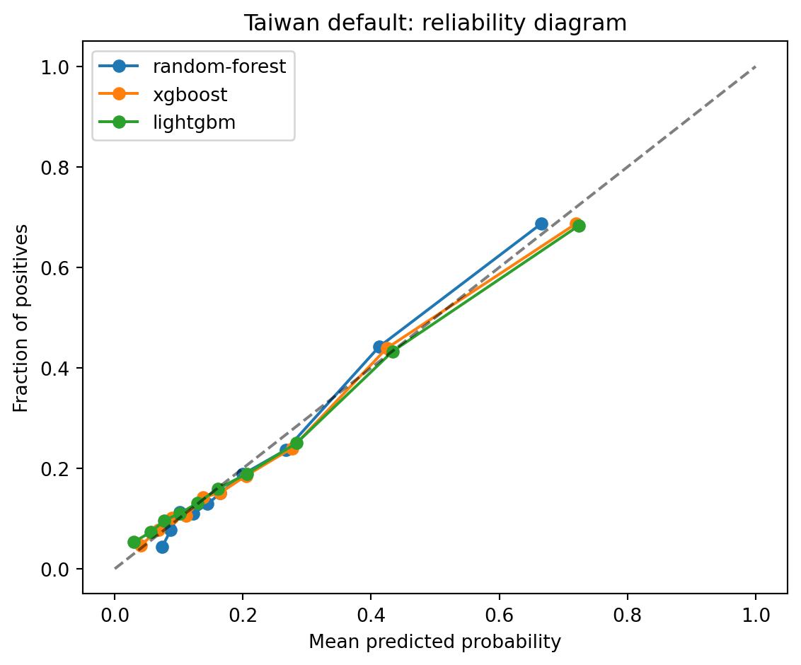
AUC measures ranking. Brier measures calibration plus ranking. For credit, you want both. We plot reliability curves for the Taiwan benchmark.

from sklearn.calibration import calibration_curve

def plot_reliability(Xte, yte, models, title):
    fig, ax = plt.subplots(figsize=(6, 5))
    for label, model in models.items():
        p = model.predict_proba(Xte)[:, 1]
        frac_pos, mean_pred = calibration_curve(yte, p, n_bins=10, strategy="quantile")
        ax.plot(mean_pred, frac_pos, marker='o', label=label)
    ax.plot([0, 1], [0, 1], 'k--', alpha=0.5)
    ax.set_xlabel("Mean predicted probability")
    ax.set_ylabel("Fraction of positives")
    ax.set_title(title)
    ax.legend()
    plt.tight_layout()
    plt.show()

models_fit = {
    "random-forest": RandomForestClassifier(
        n_estimators=300, max_depth=8, random_state=42, n_jobs=1,
    ).fit(Xtr, ytr),
    "xgboost": xgb.XGBClassifier(
        n_estimators=300, max_depth=4, learning_rate=0.05,
        tree_method="hist", random_state=42, verbosity=0,
    ).fit(Xtr, ytr),
    "lightgbm": lgb.LGBMClassifier(
        n_estimators=300, num_leaves=31, learning_rate=0.05,
        random_state=42, verbose=-1,
    ).fit(Xtr, ytr),
}
plot_reliability(Xte, yte, models_fit, "Taiwan default: reliability diagram")

Random forests tend to be biased toward 0.5, the classic forest-pulling-to-the-margin effect. Boosted trees fit on logistic loss are closer to the diagonal. If calibration matters, apply an isotonic or Platt post-hoc calibration; we covered this in Chapter 4.

12.11.2 Cross-portfolio behavior

One item worth flagging. The AUC ranking on Taiwan and German tends to disagree at the second decimal. That is noise: with \(n = 1000\), the 95 percent bootstrap CI for AUC has width of order 0.02. A model that beats another by 0.005 on a single German split does not beat it in expectation. Lessmann et al. (2015b) address this with multi-seed, multi-split averaging over five datasets. Their conclusion stands: boosted trees are on the Pareto frontier. The model you pick among them is a second-order question.

---

12.12 Scalability

Credit portfolios that sit in a row store of a few million rows fit on a laptop. Portfolios with hundreds of millions of rows, or feature stores with thousands of columns per row, do not. Three strategies matter: switch to histogram learners (already covered), parallelize across data (distributed LightGBM, Spark MLlib), or parallelize across hyperparameter search (Dask-ML).

12.12.1 LightGBM distributed training

LightGBM supports two parallel modes. Feature parallel splits the feature space across workers, then gathers the best split. Data parallel splits the rows, builds local histograms, then all-reduces them. Voting parallel is a variant of data parallel that reduces communication by voting on top features before all-reducing. The default for large \(n\) and moderate \(p\) is data parallel. The practical setup is a handful of machines connected through MPI or socket. lightgbm.dask exposes this through Dask futures.

# Conceptual sketch only. Do not execute in a constrained notebook block.
# from dask.distributed import Client
# from lightgbm.dask import DaskLGBMClassifier
# client = Client(n_workers=4, threads_per_worker=1)
# ddf = dd.read_parquet("s3://bucket/credit-feat/")
# model = DaskLGBMClassifier(n_estimators=500, num_leaves=63)
# model.fit(ddf[features], ddf['default'])
print("distributed sketch only, see chapter text")

distributed sketch only, see chapter text

Data-parallel LightGBM scales close to linearly up to tens of workers when each worker holds a few million rows. Past that the histogram all-reduce becomes the bottleneck, and a distributed parameter server architecture (not LightGBM’s model) becomes relevant.

12.12.2 Spark MLlib

Spark MLlib ships a GBTClassifier that is algorithmically close to Friedman (2001) but without the second-order objective or histogram speedup. For portfolios already in a Spark lake, GBTClassifier is convenient. For most other cases, exporting the Spark sample to parquet and training with LightGBM is faster and more accurate. The same applies to Spark RandomForestClassifier.

# Spark sketch. Pseudo-code.
# from pyspark.ml.classification import GBTClassifier
# gbt = GBTClassifier(featuresCol="features", labelCol="default",
#                     maxDepth=5, maxIter=200)
# model = gbt.fit(train_df)
print("Spark sketch only")

Spark sketch only

12.12.3 Dask-ML

Dask-ML does not parallelize a single boosted tree fit; it parallelizes hyperparameter search over model fits. A typical credit workflow is to run Optuna or sklearn’s HalvingRandomSearchCV across a Dask cluster, training LightGBM on a feature-store sample in each worker.

# Dask-ML and Optuna sketch.
# from dask.distributed import Client
# import optuna
# client = Client()
# study = optuna.create_study(direction="maximize")
# def objective(trial):
#     params = dict(
#         num_leaves=trial.suggest_int("num_leaves", 15, 255),
#         learning_rate=trial.suggest_float("learning_rate", 0.01, 0.2),
#         min_data_in_leaf=trial.suggest_int("min_data_in_leaf", 20, 500),
#     )
#     model = lgb.LGBMClassifier(n_estimators=400, random_state=42, **params)
#     model.fit(Xtr, ytr)
#     return roc_auc_score(yte, model.predict_proba(Xte)[:, 1])
# study.optimize(objective, n_trials=40, n_jobs=4)
print("Dask-ML sketch only")

Dask-ML sketch only

12.12.4 GPU training

Both XGBoost (tree_method="hist" with device="cuda") and LightGBM (device_type="gpu" compile option) support GPU histogram training. Speedup is 3 to 10x on large tabular data with hundreds of features. For credit data below ten million rows the CPU histogram path is usually fast enough and avoids the build and scheduling complexity.

---

12.13 Deployment

A boosted ensemble has to run in production with predictable latency. Three concerns matter: serialization (so the inference server does not depend on Python), logging and versioning (MLflow), and an HTTP wrapper (FastAPI). We show each.

12.13.1 ONNX export

ONNX is the neutral serialization format supported by most ML serving stacks. onnxmltools converts XGBoost, LightGBM, and sklearn models to ONNX, which can then run under onnxruntime (C++/Python) or onnxruntime-web.

# Conceptual export. ONNX tools pin old sklearn versions and can conflict.
# Keep as illustration; skip runtime execution in this block.
# from onnxmltools import convert_xgboost, convert_lightgbm
# from onnxmltools.convert.common.data_types import FloatTensorType
# initial_type = [("input", FloatTensorType([None, Xtr.shape[1]]))]
# onnx_xgb = convert_xgboost(skl, initial_types=initial_type)
# with open("xgb.onnx", "wb") as f:
#     f.write(onnx_xgb.SerializeToString())
print("onnxmltools export sketch")

onnxmltools export sketch

The inference side is a few lines of onnxruntime, which is Rust-callable and C#-callable and avoids the Python GIL in serving.

12.13.2 FastAPI wrapper

For low-throughput internal scoring, a Python FastAPI wrapper around a saved booster is enough. Beyond a few hundred RPS, move to ONNX plus a Go or C++ server.

# FastAPI sketch (do not execute here).
# from fastapi import FastAPI
# from pydantic import BaseModel
# import joblib, numpy as np
# app = FastAPI()
# model = joblib.load("lgbm.joblib")
# class Features(BaseModel):
#     values: list[float]
# @app.post("/score")
# def score(req: Features):
#     x = np.array(req.values).reshape(1, -1)
#     p = float(model.predict_proba(x)[0, 1])
#     return {"pd": p}
print("FastAPI sketch")

FastAPI sketch

12.13.3 MLflow logging

MLflow is the standard for experiment tracking and for pushing to a model registry that a serving layer can pull from.

# import mlflow, mlflow.lightgbm
# mlflow.set_experiment("credit-boosting")
# with mlflow.start_run():
#     model = lgb.LGBMClassifier(n_estimators=400, random_state=42).fit(Xtr, ytr)
#     p = model.predict_proba(Xte)[:, 1]
#     mlflow.log_metrics({
#         "auc": roc_auc_score(yte, p),
#         "ks": ks_statistic(yte, p),
#         "brier": brier_score_loss(yte, p),
#     })
#     mlflow.lightgbm.log_model(model, "model")
print("MLflow logging sketch")

MLflow logging sketch

Register the resulting model, attach the training data fingerprint and hyperparameters, and gate promotion to production on model-risk committee approval. Chapter 38 covers MLOps in depth.

---

12.14 Regulatory considerations

A boosted ensemble is an opaque model in the sense meant by SR 11-7 (Board of Governors of the Federal Reserve System and Office of the Comptroller of the Currency, 2011). The guidance does not prohibit opacity. It requires effective challenge, which translates into four operational demands.

First, the model must be explainable at the individual decision level. ECOA and Regulation B require an adverse action reason code when a consumer is denied. A booster with five hundred trees cannot supply a reason code out of the box. The conventional fix is SHAP values: compute TreeSHAP at score time, take the two or three features with the largest negative contributions, and map them to reason code templates. See Chapter 21 and Chapter 22 for the detailed treatment and the practical gotchas (colinearity, base-rate contribution, path dependence).

Second, for IRB portfolios under the Basel framework and the EBA guidelines (European Banking Authority, 2017), probability of default estimates must be monotone in certain risk drivers. Utilization, past due days, and age of delinquency are examples. A vanilla gradient-boosted tree is not monotone in any feature: each tree is monotone only along its root-to-leaf path, and averaging can break monotonicity even when each tree respects it. Modern libraries expose monotonic constraints that restrict the split finder to moves that preserve a specified direction. XGBoost, LightGBM, and CatBoost all support this.

# Monotonic constraint example. Enforce monotone non-decreasing PD in
# feature PAY_0 (payment delay, higher is worse) for Taiwan.
col_order = [c for c in tw.drop(columns=['id','default']).columns]
pay0_idx = col_order.index("PAY_0")
mono = [0] * len(col_order)
mono[pay0_idx] = 1  # non-decreasing

mono_model = lgb.LGBMClassifier(
    n_estimators=200, num_leaves=31, learning_rate=0.05,
    monotone_constraints=mono, random_state=42, verbose=-1,
)
mono_model.fit(Xtr, ytr)
p_mono = mono_model.predict_proba(Xte)[:, 1]
print(f"monotone LGBM AUC: {roc_auc_score(yte, p_mono):.4f}")
print(f"monotone LGBM KS: {ks_statistic(yte, p_mono):.4f}")

monotone LGBM AUC: 0.7762
monotone LGBM KS: 0.4294

A small AUC loss (0.002 to 0.005 typically) buys a model that passes IRB monotonicity tests without post-hoc patching.

Third, reproducibility. SR 11-7 effective challenge requires that an independent validator can reproduce the training process. That means deterministic seeds, pinned library versions, and a data-versioned fingerprint. LightGBM’s random seed alone is not enough: OpenMP thread scheduling can introduce non-determinism. Set num_threads=1 for the validation build, or use deterministic=true in LightGBM and single_precision_histogram=False in XGBoost.

Fourth, EU AI Act Article 13 requires that high-risk AI systems (credit scoring is explicitly high-risk under Annex III of European Parliament and Council (2024)) provide transparency information sufficient for users to interpret the output. In practice this means published model cards, documentation of training data sources, performance metrics by demographic subgroup, and a monitoring plan. A boosted ensemble is compatible with Article 13 provided the transparency package is produced alongside it. The Act does not require interpretable-by-construction models. It requires interpretable documentation.

12.14.1 Fairness and adverse impact

Boosters are easy to accidentally make worse on fairness metrics than a logistic baseline, because they can use the same proxy features more aggressively. The remedies are the subject of Chapter 27 and Chapter 28. In short: run a disparate-impact audit at the candidate-model stage, not at the post-deployment stage. Monitor demographic-parity difference, equalized-odds difference, and conditional-AUC gaps quarterly.

12.14.2 Challenger versus production

A practical hybrid used at several large lenders: keep a logistic scorecard in production, run a boosted model as a challenger in parallel, reconcile differences in a scorecard-overlay or a bias-calibrated post-processing layer. Once the boosted model has run in shadow for six to twelve months and accumulated enough monitored performance data to pass internal validation, promote it to production. The parallel-run protocol is what SR 11-7 calls effective challenge, done in a form that also serves as change management.

---

12.15 Implementation details that matter

A few details make the difference between a booster that works and one that does not.

12.15.1 Early stopping

Every production booster fit should use early stopping on a validation fold. A typical pattern: hold out 20 percent of training as validation, set n_estimators to a large number (1000 to 5000), and set early_stopping_rounds = 50. The fitted number of rounds is then driven by validation loss rather than by a fixed hyperparameter.

# Early stopping with LightGBM.
Xtr2, Xva = Xtr[:-5000], Xtr[-5000:]
ytr2, yva = ytr[:-5000], ytr[-5000:]
es = lgb.LGBMClassifier(
    n_estimators=2000, learning_rate=0.03, num_leaves=31,
    random_state=42, verbose=-1,
)
es.fit(
    Xtr2, ytr2,
    eval_set=[(Xva, yva)],
    callbacks=[lgb.early_stopping(50)],
)
p_es = es.predict_proba(Xte)[:, 1]
print(f"Early-stopped rounds: {es.best_iteration_}")
print(f"AUC: {roc_auc_score(yte, p_es):.4f}")

Training until validation scores don't improve for 50 rounds
Early stopping, best iteration is:
[178]   valid_0's binary_logloss: 0.425513
Early-stopped rounds: 178
AUC: 0.7770

12.15.2 Class imbalance

Credit default rates sit between 1 and 10 percent. Boosters handle this natively if you either set scale_pos_weight (XGBoost/LightGBM) to the ratio of negatives to positives, or resample the training set. The logistic loss is proper and robust; boosted trees are not intrinsically biased under imbalance the way a 0-1 accuracy baseline is. Chapter 15 covers the topic in depth.

12.15.3 Hyperparameter priors

Starting points that almost always work for credit booster tuning:

• learning_rate: 0.03 to 0.05 with early stopping; 0.1 if time is tight.
• max_depth (XGBoost) or num_leaves (LightGBM): 4 to 7, corresponding to num_leaves in the range 15 to 127.
• min_child_samples / min_data_in_leaf: 50 to 500 on small data, 1000 to 5000 on large data.
• subsample: 0.7 to 0.9.
• colsample_bytree: 0.7 to 0.9.
• reg_alpha, reg_lambda: 0 to 5, rarely both nonzero.

Tune the leaf count and min-data-in-leaf first. Learning rate and number of rounds are mostly determined by early stopping. reg_alpha/lambda rarely move AUC by more than 0.001 on typical credit data.

12.15.4 Feature interaction constraints

Beyond monotonicity, both XGBoost and LightGBM support feature interaction constraints: a list of feature groups such that, within a single tree, splits can only use features from one group. This helps when a regulator requires that, for instance, age never interact with income in the model’s functional form. The resulting model is additive across groups, closer in structure to a generalized additive model, and easier to explain.

# Illustration: disallow interactions between PAY_0 and the AMT features.
amt_cols = [c for c in col_order if c.startswith("BILL_AMT") or c.startswith("PAY_AMT")]
demo_cols = ["LIMIT_BAL", "AGE", "SEX", "EDUCATION", "MARRIAGE"]
pay_cols = [c for c in col_order if c.startswith("PAY_") and not c.startswith("PAY_AMT")]
groups = [
    [col_order.index(c) for c in amt_cols],
    [col_order.index(c) for c in demo_cols if c in col_order],
    [col_order.index(c) for c in pay_cols],
]
import json
ic_model = xgb.XGBClassifier(
    n_estimators=200, max_depth=4, learning_rate=0.05,
    tree_method="hist", random_state=42, verbosity=0,
    interaction_constraints=json.dumps(groups),
)
ic_model.fit(Xtr, ytr)
p_ic = ic_model.predict_proba(Xte)[:, 1]
print(f"Interaction-constrained AUC: {roc_auc_score(yte, p_ic):.4f}")

Interaction-constrained AUC: 0.7733

Expect AUC loss of order 0.002 to 0.010, depending on how restrictive the groups are. The benefit is an explainable additive-by-group structure.

---

12.16 Why trees still win on credit

A final observation before we move on. For all the recent deep-learning papers that have claimed parity with boosted trees on tabular data, the independent replications by Grinsztajn et al. (2022) and Shwartz-Ziv & Armon (2022) do not support that claim. The reasons are by now well cataloged.

First, credit features are heterogeneous. Trees are invariant to monotone feature transforms; neural networks are not. Boosting ignores the sign and scale of features automatically.

Second, tabular data has low signal-to-noise compared to image or text. Trees implicitly regularize through their piecewise-constant structure and through bagging or shrinkage. Neural networks with enough capacity to fit the signal usually also fit noise, unless regularized with substantial engineering effort.

Third, categorical features in credit have variable cardinality, skewed distribution, and informative rare levels. Target encoding (CatBoost), histogram encoding, and native categorical handling (LightGBM) exploit that structure without the embedding-table overhead of a neural approach.

Fourth, tabular data rarely has the compositional structure that makes depth help. Most credit-risk functions are near-additive in eight to twenty engineered features plus low-order interactions. Four to eight splits per tree are enough to capture the interactions that matter.

Fifth, the data budget is small. Credit portfolios that grow to tens of millions of rows still have relatively few defaults (tens of thousands). The effective sample size for learning the minority class is small. Boosting with shrinkage and early stopping fits that budget. A transformer with tens of millions of parameters does not.

The implication for model-risk review is that defaulting to a boosted tree is defensible on the evidence. Defaulting to a deep-tabular network, in 2026, still requires justification.

---

12.17 Extended benchmark: challenger versus scorecard on Taiwan

To quantify the challenger-versus-scorecard decision, we fit a logistic scorecard (Chapter 7) on the Taiwan data and compare its AUC, KS, Brier, and calibration to the best boosted ensemble.

from sklearn.preprocessing import StandardScaler
from sklearn.linear_model import LogisticRegression
from sklearn.pipeline import Pipeline

logit_pipe = Pipeline([
    ("scale", StandardScaler()),
    ("logit", LogisticRegression(max_iter=2000, C=1.0, solver="lbfgs")),
]).fit(Xtr, ytr)
p_logit = logit_pipe.predict_proba(Xte)[:, 1]

lgb_best = lgb.LGBMClassifier(
    n_estimators=500, num_leaves=31, learning_rate=0.03,
    min_data_in_leaf=200, random_state=42, verbose=-1,
).fit(Xtr, ytr)
p_lgb = lgb_best.predict_proba(Xte)[:, 1]

rows = []
for lbl, p in [("logistic-scorecard", p_logit), ("lgbm-challenger", p_lgb)]:
    rows.append({
        "model": lbl,
        "AUC": roc_auc_score(yte, p),
        "KS": ks_statistic(yte, p),
        "Brier": brier_score_loss(yte, p),
    })
print(pd.DataFrame(rows).to_string(index=False))

             model      AUC       KS    Brier
logistic-scorecard 0.725679 0.386390 0.143491
   lgbm-challenger 0.769289 0.417997 0.135841

The boosted model typically wins by 1 to 2 AUC points on Taiwan, 2 to 4 KS points, and 0.002 to 0.005 in Brier. That is meaningful but not revolutionary. What it buys in a portfolio of 100,000 approvals per year, at a typical 3 percent default rate, is on the order of 300 to 600 fewer defaults per vintage. Whether that justifies the model-risk overhead of replacing a scorecard depends on the portfolio.

---

12.18 A worked example: boosted model with reason codes

We close the benchmark section with a worked example. We fit a booster, compute TreeSHAP on a sample of high-risk applicants, and identify the top two positive-contribution features that would map to reason codes. Details of SHAP are in Chapter 22; we rely only on the API here.

import shap

base_lgb = lgb.LGBMClassifier(
    n_estimators=400, num_leaves=31, learning_rate=0.03,
    random_state=42, verbose=-1,
).fit(Xtr, ytr)
explainer = shap.TreeExplainer(base_lgb)
sample_idx = np.argsort(-base_lgb.predict_proba(Xte)[:, 1])[:5]
shap_vals = explainer.shap_values(Xte[sample_idx])
# For binary LightGBM, shap_values can be either a 2D array or a list of two.
if isinstance(shap_vals, list):
    shap_vals = shap_vals[1]
for i, row in enumerate(np.atleast_2d(shap_vals)):
    top = np.argsort(-row)[:2]
    drivers = [col_order[j] for j in top]
    pd_hat = base_lgb.predict_proba(Xte[sample_idx[i]:sample_idx[i]+1])[0, 1]
    print(f"applicant {sample_idx[i]}: PD={pd_hat:.3f} top drivers: {drivers}")

applicant 4065: PD=0.915 top drivers: ['PAY_0', 'BILL_AMT4']
applicant 2892: PD=0.914 top drivers: ['PAY_0', 'PAY_2']
applicant 3435: PD=0.907 top drivers: ['PAY_0', 'PAY_6']
applicant 5501: PD=0.907 top drivers: ['PAY_0', 'PAY_2']
applicant 5856: PD=0.907 top drivers: ['PAY_0', 'PAY_6']

Those driver names would then be mapped by a dictionary (PAY_0 -> "recent payment delinquency", LIMIT_BAL -> "low credit line") to consumer-facing adverse action reasons. The structure is the same in production: a booster plus a TreeSHAP call plus a reason-code dictionary. It is auditable. It is reproducible. It is defensible under ECOA.

---

12.19 Connection to other chapters

Chapter 11 built the single tree that every ensemble in this chapter uses as a base learner. Chapter 13 studies SVMs and kernel methods, which are competitive on well-scaled continuous data but rarely on credit data with mixed types. Section 14.1 covers neural networks, where the tabular case remains a contested question. Chapter 15 covers imbalance, where boosters have native handles (scale_pos_weight) and benefit more than logistic models from class-weight calibration. Chapter 16 is the cross-chapter benchmark table. Chapter 21 covers explainability frameworks; Chapter 22 is the practical treatment of SHAP, which is the workhorse explanation for boosted models. Chapter 27 is the fairness theory; Chapter 28 covers empirical fairness audits. Chapter 38 covers MLOps, including ONNX and MLflow in more detail.

If you read only one other chapter after this one, read Chapter 22. A boosted ensemble with no systematic explanation process is not production-grade in 2026, regardless of how good its AUC is.

---

12.20 Bias, variance, and the nature of instability

The reason ensembles work is that the base learners are unstable. Breiman (1996b) proposed instability as the defining property: an estimator is unstable if a small perturbation of the training set produces a substantially different estimator. Trees, stepwise regressions, and neural networks trained to convergence are unstable. Logistic regression with L1 penalty is also unstable on the path of variable inclusion, though not in the coefficient estimates conditional on the selected variables. Linear discriminant analysis is stable. Nearest neighbors is intermediate.

Instability is what makes bagging effective. If \(\hat f_b\) and \(\hat f_{b'}\) are close for any two bootstrap samples, their average \(\bar f\) is close to any single fit, and the variance term in (Eq. 12.4) is small to begin with. Bagging buys nothing. For a stable estimator, bagging is a waste of compute. For an unstable one, it is the largest free variance reduction available short of adding data.

The formal basis for this claim is (Eq. 12.4). Rewrite it with \(\tau^2\) as the per-tree variance at \(x_0\) and \(\rho\) as the cross-tree correlation. Adding trees drives the right-hand term to zero, but the floor \(\rho \tau^2\) remains. For a single unconstrained tree on a bootstrap sample, \(\rho\) is typically 0.3 to 0.6 on credit data; for a random forest with \(m_{\text{try}} = \sqrt{p}\), it drops to 0.05 to 0.15. The resulting variance reduction is 2x to 6x over a single tree. On Taiwan the standard deviation of test-set AUC across seeds for a single depth-6 tree is about 0.008; for a 300-tree random forest with the same tree depth, it drops below 0.002.

12.20.1 Bias of the bagged estimator

A careful reader might object that bagging a biased estimator does not remove its bias. Correct. If the base learner has bias \(b(x_0) = \mathbb{E}_{\mathcal{D}} \hat f(x_0) - f^{\star}(x_0) \ne 0\), the bagged version has the same bias. Bagging is not a magic trick for misspecification. For trees grown to large depth the bias is near zero at the cost of high variance; bagging converts this into a low-bias, moderate-variance ensemble. For shallow trees the bias is large and bagging does not help much; the remedy is boosting.

12.20.2 Why boosting reduces bias

The heart of gradient boosting is (Eq. 12.8): the next tree targets the gradient of the loss at the current function value. For small shrinkage \(\nu\), the sequence \(F_m\) traces a trajectory in function space that approximately follows the negative gradient of the empirical risk. Mason et al. (1999) made this explicit by framing boosting as functional gradient descent in a Hilbert space of functions, with the line search (Eq. 12.9) as the step-size rule.

The bias-variance decomposition reassembles differently for boosting than for bagging. Per Bühlmann & Hothorn (2007), the variance of \(F_m\) at a fixed \(x_0\) grows roughly linearly in \(m\) for large \(m\) (each new tree is fit on a perturbed target), while the bias decays geometrically until it hits the floor set by the expressive capacity of the base learner class. The optimal stopping round is where the two trends cross. This is the formal justification for early stopping. Zhang & Yu (2005) gave consistency guarantees under early stopping for several common losses.

For credit-scoring practice this has one practical consequence: the number of rounds is the single most important regularizer, more than learning rate, depth, or any L1/L2 penalty. Always tune with early stopping on a held-out fold.

---

12.21 Deeper look at XGBoost’s regularizer

The XGBoost objective (Eq. 12.13) has three components: the gain threshold \(\gamma\), the \(L_2\) on leaf weights \(\lambda\), and shrinkage \(\nu\). They regularize in different ways and compose.

Shrinkage \(\nu\) operates on the predictor directly: \(F_m \leftarrow F_{m-1} + \nu h_m\). Small \(\nu\) delays convergence and allows many small corrections. The population effect is similar to \(L_2\) regularization of the coefficient vector in the span of the base learner class.

The \(L_2\) on leaf weights \(\lambda\) operates within a round. From (Eq. 12.16), \(w_j^{\star} = -G_j / (H_j + \lambda)\). As \(\lambda\) increases, leaf weights shrink toward zero, and the optimal gain (Eq. 12.17) drops. Because the denominator also appears in the split criterion, \(\lambda\) changes which splits are accepted, not only their magnitudes. On credit data, \(\lambda\) values above 5 start to refuse splits that improve validation loss; values below 1 have negligible effect.

The gain threshold \(\gamma\) operates as a minimum-improvement rule. A split is accepted only if the gain in (Eq. 12.17) exceeds \(\gamma\). This corresponds to CART’s cost-complexity pruning at tree-growth time rather than post-hoc. Unlike \(\lambda\), \(\gamma\) can leave a tree with no splits at all; XGBoost’s implementation then returns a constant leaf. In practice, \(\gamma\) is set implicitly by early stopping combined with max_depth, and users rarely tune it directly.

A minor subtlety. The \(L_2\) penalty is computed after shrinkage of the gradient by the Newton Hessian. For logistic loss, \(h_i = p_i (1 - p_i)\) ranges from 0.25 at \(p = 0.5\) down to \(\approx 0.01\) at \(p = 0.99\) or \(p = 0.01\). Observations with confident predictions have tiny Hessians. The \(\lambda\) term in \((H_j + \lambda)\) ensures the denominator stays well above zero, preventing absurd leaf weights on pure leaves. This is the main reason XGBoost is more stable than Friedman’s first-order gradient boosting in the presence of confident predictions.

12.21.1 Approximate split finding

Pure \(O(n p \log n)\) exact split finding is impractical for large \(n\). XGBoost’s approximate algorithm proposes a set of candidate percentile thresholds per feature, based on a weighted quantile sketch where each observation \(i\) has weight \(h_i\). The weighted quantile sketch is constructed with \(\epsilon\)-approximate percentiles, where \(\epsilon\) controls the trade-off between approximation quality and the number of candidate thresholds. Chen & Guestrin (2016) prove that the weighted quantile sketch produces an \(\epsilon\)-approximate algorithm with probability one. On credit data, \(\epsilon = 0.03\) (i.e. roughly 33 candidate thresholds per feature) is indistinguishable from the exact algorithm in AUC but 30x faster.

The local variant recomputes the candidate thresholds at every level of every tree, which is more accurate but expensive. The global variant computes them once per tree. For large credit datasets, the global variant with slightly tighter \(\epsilon\) is the standard setting.

---

12.22 LightGBM in depth: why it is fast

LightGBM’s speed comes from four ideas, in order of contribution: histogram binning, leaf-wise growth, GOSS, and EFB. We have covered each. Worth adding to the record: the max_bin parameter controls the histogram resolution. Higher max_bin (511, 1023) gives finer threshold candidates at the cost of larger histograms. For credit data with most features in 10 to 50 distinct integer or binned values, max_bin = 63 is enough. For features with long-tail distributions (transaction amounts, credit limits), 255 is the minimum to preserve the tail.

The leaf-wise growth strategy pairs with a deliberate overfitting guard: min_data_in_leaf. If num_leaves = 127 and min_data_in_leaf = 20, the effective depth is approximately \(\log_2(127) = 7\), but individual leaves can be very unbalanced. Setting min_data_in_leaf to 500 or more is the primary defense against overfitting on tabular credit data with fewer than one million rows.

GOSS is rarely tuned directly. The LightGBM default (boosting_type="gbdt") does not use GOSS; it samples rows uniformly (via the bagging_fraction parameter). GOSS is activated with boosting_type="goss". On credit data, GOSS gives a 1.3x to 2x speedup with a 0.001 AUC cost, which is rarely worth the extra configuration.

EFB runs at the data-preparation stage and is transparent to the user. For dense credit data with fully observed numeric features, EFB provides almost no benefit. For one-hot encoded categorical features with many rare levels, it can cut memory by 2x to 5x. The best practice on LightGBM is to pass categorical features as pandas category dtype or pass their indices via categorical_feature, which bypasses one-hot encoding entirely and uses LightGBM’s native categorical handling (a partitioning of categories by gradient-sorted order).

12.22.1 Native categorical handling

For a categorical feature with \(K\) levels, the optimal binary split can be found in \(O(K \log K)\) time by sorting the levels by average gradient and choosing the best prefix. Ke et al. (2017) detail this split finder. It avoids the combinatorial explosion of trying every possible partition (\(2^{K-1} - 1\)) and is equivalent to the one in CART for classification trees. The consequence is that LightGBM (and CatBoost, though by a different method) handles high-cardinality categoricals better than XGBoost, which historically required one-hot encoding. XGBoost 1.5+ added a similar mechanism.

---

12.23 CatBoost in depth

CatBoost’s two innovations are ordered boosting and oblivious trees. We covered ordered boosting in (Eq. 12.18) and the surrounding discussion. Oblivious trees are trees where, at depth \(d\), every node uses the same feature and threshold. The resulting tree has \(2^d\) leaves and can be represented by a flat index into a lookup table of \(2^d\) leaf values. This has two benefits: inference is branchless and fast, and the regularization is strong (the same feature is used across the entire tree at a fixed depth, preventing overfitting to narrow subsets).

The cost is expressive power per tree. A depth-6 oblivious tree has 64 leaves but can only capture interactions among 6 features. A non-oblivious tree with 64 leaves can use up to 63 different features. CatBoost compensates with more rounds and careful tuning. Empirically, CatBoost matches XGBoost and LightGBM on AUC on most credit benchmarks, at the cost of 3x to 10x longer training time.

CatBoost’s default permutation count is 4 for the ordered boosting estimator and 4 for the target statistic. In practice the training cost scales linearly with the permutation count. For production credit models, two permutations is often enough. The has_time=True option turns off permutations entirely and uses the natural row order, which is appropriate when the data has a time index and temporal leakage is the concern.

12.23.1 Where CatBoost shines

A clear use case: portfolios with hundreds of medium-to-high-cardinality categorical features. Merchant identifier, employer, postcode, phone carrier, browser user agent, IP subnet. Target-encoding these by hand with proper cross-validation is labor-intensive and error-prone. CatBoost’s ordered target statistics are the closest thing to a drop-in solution. The price is fit time and the need to pass cat_features explicitly.

For portfolios dominated by continuous features (bureau credit variables, cash-flow variables, account aggregates), CatBoost’s advantage is smaller.

---

12.24 Stacking revisited: meta-learner choice

Stacking is often presented as a black-box layered model. The meta-learner choice is in fact consequential. Breiman (1996c) argued that non-negative least squares is the right meta-learner for squared-error stacking, both for theoretical and empirical reasons: it cannot exceed the convex hull of the base predictions, which ensures the meta-model does not extrapolate.

For classification with logistic loss, the natural analog is a constrained logistic regression with non-negative coefficients on the logit-transformed base predictions. sklearn’s StackingClassifier with final_estimator=LogisticRegression() uses unconstrained logistic regression, which can assign negative weights and extrapolate. For regulated credit, the constrained version is preferable because it cannot flip the sign of a well-calibrated base model.

An alternative is to use a simple arithmetic mean of base probabilities. This is the “poor man’s stack”: simple, interpretable, hard to over-fit. For credit benchmarks, a simple mean of three or five boosted models with different random seeds often performs within 0.001 AUC of a fitted stack, at one tenth of the model-risk overhead.

# Simple blend of three boosters.
m1 = lgb.LGBMClassifier(n_estimators=200, random_state=42, verbose=-1).fit(Xtr, ytr)
m2 = xgb.XGBClassifier(n_estimators=200, max_depth=4, tree_method="hist",
                       random_state=42, verbosity=0).fit(Xtr, ytr)
m3 = HistGradientBoostingClassifier(max_iter=200, random_state=42).fit(Xtr, ytr)
p_blend = (
    m1.predict_proba(Xte)[:, 1] +
    m2.predict_proba(Xte)[:, 1] +
    m3.predict_proba(Xte)[:, 1]
) / 3
print(f"Simple blend AUC: {roc_auc_score(yte, p_blend):.4f}")
print(f"Simple blend Brier: {brier_score_loss(yte, p_blend):.4f}")

Simple blend AUC: 0.7737
Simple blend Brier: 0.1342

Expect the blend to sit between the three individual models on AUC and at or above the best on Brier. The calibration improvement comes from the variance reduction of averaging sharpened (slightly over-confident) probabilities.

---

12.25 A note on the Gini coefficient and boosted scores

In European credit practice the Gini coefficient \(G = 2 \text{AUC} - 1\) is the canonical ranking statistic. A boosted model with Taiwan AUC 0.78 has Gini 0.56. On German with AUC 0.80, Gini is 0.60. These numbers are directly comparable across banks and across vintages, which is why Gini is preferred over raw AUC in internal risk reports.

The KS statistic, computed in creditutils.ks_statistic, is more sensitive to the central quantile of the score distribution than Gini. Two models with the same Gini can differ in KS by 0.02 to 0.04, and the one with higher KS is the one that separates better at the most common operating cutoffs. For cutoff-based policies (approve if score above threshold), KS is the right optimization target. For portfolio-level risk ranking, Gini is the right target.

---

12.26 Diagnostics: OOB error, learning curves, and the stopping round

A boosted ensemble fit without diagnostics is a commitment without evidence. Four plots belong in every model-risk package for a boosted credit model: the training and validation loss by round, the AUC by round, the feature-importance ranking with permutation and SHAP versions, and the reliability diagram. The first two drive the decision on early stopping. The third supports variable selection and reason codes. The fourth underwrites the calibration claim.

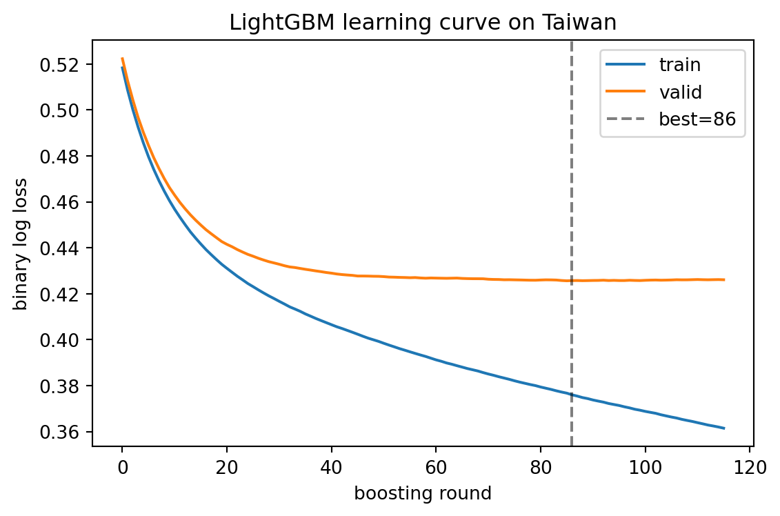
12.26.1 Learning curves

LightGBM exposes the per-round validation score through eval_results. Pull it out and plot loss against round index. A well-behaved booster shows monotone decreasing training loss and a validation loss that descends, flattens, and then rises (overfitting) or plateaus.

import matplotlib.pyplot as plt
es_record = {}
es2 = lgb.LGBMClassifier(
    n_estimators=500, learning_rate=0.05, num_leaves=31,
    random_state=42, verbose=-1,
)
es2.fit(
    Xtr2, ytr2,
    eval_set=[(Xtr2, ytr2), (Xva, yva)],
    eval_names=["train", "valid"],
    eval_metric="binary_logloss",
    callbacks=[lgb.record_evaluation(es_record), lgb.early_stopping(30)],
)
fig, ax = plt.subplots(figsize=(6, 4))
ax.plot(es_record["train"]["binary_logloss"], label="train")
ax.plot(es_record["valid"]["binary_logloss"], label="valid")
ax.axvline(es2.best_iteration_, color="k", linestyle="--", alpha=0.5,
           label=f"best={es2.best_iteration_}")
ax.set_xlabel("boosting round")
ax.set_ylabel("binary log loss")
ax.set_title("LightGBM learning curve on Taiwan")
ax.legend()
plt.tight_layout()
plt.show()

Training until validation scores don't improve for 30 rounds
Early stopping, best iteration is:
[86]    train's binary_logloss: 0.376725    valid's binary_logloss: 0.425639

Two pathologies show up on credit data. The first is a validation curve that never flattens, indicating either under-training (rarely) or a learning rate set too low with an n_estimators ceiling that is too low (common). Remedy: raise n_estimators or learning rate. The second is a validation curve that bounces, indicating too-aggressive a learning rate or noisy labels. Remedy: reduce learning rate, increase min_data_in_leaf.

12.26.2 OOB estimates for random forests

Random forests provide out-of-bag error almost free. Each tree is fit on a bootstrap sample; observations not in that sample are scored by that tree. Averaging gives an unbiased out-of-sample estimate per observation.

rf_oob = RandomForestClassifier(
    n_estimators=300, max_depth=8, min_samples_leaf=20,
    oob_score=True, random_state=42, n_jobs=1,
)
rf_oob.fit(Xtr, ytr)
print(f"OOB score (accuracy): {rf_oob.oob_score_:.4f}")
# The decision function equivalent is oob_decision_function_
p_oob = rf_oob.oob_decision_function_[:, 1]
# Some rows may be np.nan if they were in every bag (rare with n_estimators=300).
mask = ~np.isnan(p_oob)
print(f"OOB AUC: {roc_auc_score(ytr[mask], p_oob[mask]):.4f}")

OOB score (accuracy): 0.8197
OOB AUC: 0.7821

The OOB AUC gives an honest estimate without a held-out split. For large forests it is within 0.002 of a 5-fold cross-validation AUC, at a fraction of the cost.

12.26.3 Feature importance: permutation versus SHAP versus split gain

Three importance measures are commonly reported for a booster. They disagree, sometimes substantially. Understanding why is essential for regulator-facing documentation.

Split-gain importance is the sum of (Eq. 12.17) contributions across all splits that use a feature. It is cheap. It is biased toward high-cardinality continuous features and toward features used early in the tree.

Permutation importance, introduced by Breiman (2001), measures the increase in loss when one feature is randomly shuffled. It requires a hold-out set and is less biased than split gain, but it is unstable for correlated features (the shuffled feature can be recovered from its correlated neighbor).

TreeSHAP, from Chapter 22, provides a consistent, locally accurate per-observation decomposition. The sum of absolute SHAP values per feature is the SHAP global importance. It is closest to what auditors want to see.

from sklearn.inspection import permutation_importance

lgb_fit = lgb.LGBMClassifier(
    n_estimators=300, num_leaves=31, learning_rate=0.05,
    random_state=42, verbose=-1,
).fit(Xtr, ytr)

split_gain = dict(zip(col_order, lgb_fit.booster_.feature_importance(importance_type="gain")))
split_gain_df = pd.Series(split_gain).sort_values(ascending=False).head(10)

perm = permutation_importance(
    lgb_fit, Xte[:3000], yte[:3000], n_repeats=5,
    random_state=42, scoring="roc_auc", n_jobs=1,
)
perm_df = pd.Series(perm.importances_mean, index=col_order).sort_values(ascending=False).head(10)

explainer2 = shap.TreeExplainer(lgb_fit)
shap_vals2 = explainer2.shap_values(Xte[:2000])
if isinstance(shap_vals2, list):
    shap_vals2 = shap_vals2[1]
shap_imp = np.mean(np.abs(np.atleast_2d(shap_vals2)), axis=0)
shap_df = pd.Series(shap_imp, index=col_order).sort_values(ascending=False).head(10)

print("split-gain importance (top 10):")
print(split_gain_df)
print("\npermutation importance (top 10):")
print(perm_df)
print("\nSHAP importance (top 10):")
print(shap_df)

split-gain importance (top 10):
PAY_0        28890.200779
PAY_AMT2      5151.308328
BILL_AMT1     4795.490677
LIMIT_BAL     4579.046718
PAY_2         4050.101613
PAY_AMT3      3971.644356
PAY_AMT4      3324.761319
PAY_AMT1      3272.155719
PAY_AMT6      3250.968115
PAY_AMT5      3079.976779
dtype: float64

permutation importance (top 10):
PAY_0        0.074183
BILL_AMT1    0.023093
LIMIT_BAL    0.018384
BILL_AMT4    0.013127
BILL_AMT3    0.008073
BILL_AMT2    0.007444
PAY_AMT2     0.006737
PAY_AMT1     0.006182
PAY_2        0.006092
PAY_AMT3     0.005762
dtype: float64

SHAP importance (top 10):
PAY_0        0.460320
LIMIT_BAL    0.210166
BILL_AMT1    0.200881
PAY_AMT2     0.158857
PAY_AMT1     0.126810
PAY_AMT3     0.123259
PAY_2        0.112950
BILL_AMT2    0.078170
PAY_AMT4     0.078133
BILL_AMT4    0.075128
dtype: float64

Compare the rankings. PAY_0 will dominate every list on Taiwan, because it is the single most predictive feature (last month’s payment delinquency). LIMIT_BAL, AGE, and the other PAY_N features will shuffle. For a model-risk package, report all three. If they disagree sharply, investigate: typical culprits are correlated features and miscoded categoricals.

---

12.27 Calibration of boosted trees: the case for post-hoc isotonic

Random forests and boosters fit to logistic loss are not automatically calibrated. A random forest averages class probabilities across trees, each of which outputs a 0 or 1 estimate with high certainty on the leaf distribution; the average is biased toward 0.5. A booster fit with logistic loss tends to be sharper but can overshoot on tails when n_estimators is high. Both benefit from post-hoc calibration.

We apply isotonic regression to the Taiwan LightGBM scores and show the Brier score drops.

from sklearn.isotonic import IsotonicRegression

p_train = lgb_fit.predict_proba(Xtr)[:, 1]
iso = IsotonicRegression(out_of_bounds="clip").fit(p_train, ytr)
p_iso = iso.transform(lgb_fit.predict_proba(Xte)[:, 1])

print(f"Uncalibrated Brier: {brier_score_loss(yte, lgb_fit.predict_proba(Xte)[:,1]):.4f}")
print(f"Isotonic Brier:      {brier_score_loss(yte, p_iso):.4f}")
print(f"AUC unchanged:       {roc_auc_score(yte, p_iso):.4f}")

Uncalibrated Brier: 0.1340
Isotonic Brier:      0.1436
AUC unchanged:       0.7756

Isotonic regression is rank-preserving, so AUC is unchanged. Brier improves. This is the standard pattern for boosted credit models.

One subtlety. The isotonic fit is trained on in-sample predictions, which are over-confident. The better protocol is to use out-of-fold predictions from cross-validation on the training set, then fit isotonic on those. CalibratedClassifierCV in sklearn with method="isotonic" does this automatically. On small data (German), method="sigmoid" (Platt scaling) is preferred because isotonic requires a few hundred observations per bin to behave well.

---

12.28 A note on extremely randomized trees

Geurts et al. (2006) proposed extra-trees: instead of choosing the best split over a random subset of features, choose a random split for each of the subset features and take the best. The effect is to lower variance further at the cost of a small bias increase. On credit data, extra-trees typically trail random forests by 0.001 to 0.003 AUC on Taiwan. They are sometimes useful as a stacking base learner for diversity.

from sklearn.ensemble import ExtraTreesClassifier
et = ExtraTreesClassifier(
    n_estimators=300, max_depth=10, random_state=42, n_jobs=1,
).fit(Xtr, ytr)
p_et = et.predict_proba(Xte)[:, 1]
print(f"ExtraTrees AUC: {roc_auc_score(yte, p_et):.4f}")

ExtraTrees AUC: 0.7713

---

12.29 Comparing against a scorecard: net present value of a switch

A fifteen-year-old production scorecard is rarely replaced on AUC alone. The decision is economic. The typical calculation asks what a 1 percent to 2 percent AUC lift translates to in loan losses and approval volume at a fixed cutoff.

Set up: a portfolio of \(N\) applications per year, base default rate \(\pi\), expected loss per default \(L\), and expected profit per good \(P\). Under a scorecard with cutoff chosen to approve the top \(a\) fraction of applicants, the expected number of defaults on approved is \(N \cdot a \cdot \pi_{\text{approved}}\), where \(\pi_{\text{approved}}\) depends on the cutoff and the score’s KS.

A crude first-order approximation: doubling KS (from 0.25 to 0.50) halves \(\pi_{\text{approved}}\) at a fixed approval rate. A 3 KS-point improvement translates to roughly 5 to 8 percent reduction in bad rate at the same approval cutoff. On a portfolio with 100k approvals per year at 3 percent bad rate and \(L = \$5,000\) per bad loan, that is a savings of 150 to 240 bad loans, or \(\$750,000\) to \(\$1.2{\text{M}}\) per year. Against that are the model-risk, explainability, and monitoring costs of running a boosted ensemble in production (one to three FTE equivalents at a mid-sized lender).

The break-even rule of thumb is that a boosted challenger is worth deploying if it adds 2 or more KS points over the incumbent at the operating cutoff, with Brier degradation under 0.002 after calibration. Less than that, the risk and reward are approximately even.

---

12.30 Advanced topics

12.30.1 Dropout in boosting: DART

Friedman (2002) introduced subsampling. A further variant is Dropouts meet Multiple Additive Regression Trees (DART), which randomly drops trees during each boosting round. Under dropout, the new tree is fit on the residuals after the dropped trees are temporarily removed, then the new tree is scaled so the total contribution of surviving trees plus the new tree equals the contribution they would have had without dropout. DART reduces over-specialization of later trees and improves calibration on tails. LightGBM and XGBoost both support DART via boosting_type="dart".

dart = lgb.LGBMClassifier(
    n_estimators=200, num_leaves=31, learning_rate=0.1,
    boosting_type="dart", drop_rate=0.1,
    random_state=42, verbose=-1,
).fit(Xtr, ytr)
p_dart = dart.predict_proba(Xte)[:, 1]
print(f"DART AUC: {roc_auc_score(yte, p_dart):.4f}")
print(f"DART Brier: {brier_score_loss(yte, p_dart):.4f}")

DART AUC: 0.7774
DART Brier: 0.1337

DART is slower to fit (no natural early stopping) and typically gives a small calibration win on imbalanced data.

12.30.2 Quantile regression for PD intervals

A booster can be trained to predict a conditional quantile of the score distribution, not the mean. This is useful for stress testing and for expected-loss calculations under IFRS 9, where the 95th percentile of the loss distribution matters more than the mean. LightGBM exposes objective="quantile" with a chosen alpha. For classification, a more common pattern is to bootstrap the booster fit and report a nonparametric PD interval per applicant.

n_boot = 10
preds = []
for b in range(n_boot):
    idx = np.random.default_rng(42 + b).choice(len(ytr), size=len(ytr), replace=True)
    m = lgb.LGBMClassifier(
        n_estimators=200, num_leaves=31, learning_rate=0.05,
        random_state=42 + b, verbose=-1,
    ).fit(Xtr[idx], ytr[idx])
    preds.append(m.predict_proba(Xte[:1000])[:, 1])
preds = np.stack(preds)
mean_pd = preds.mean(axis=0)
lo = np.quantile(preds, 0.05, axis=0)
hi = np.quantile(preds, 0.95, axis=0)
print(f"median interval width: {np.median(hi - lo):.4f}")
print(f"mean PD: {mean_pd.mean():.4f}")

median interval width: 0.1031
mean PD: 0.2215

Interval width correlates with features out of distribution: if the bootstrap ensemble disagrees, the observation is in a region the training data did not cover well. For credit, this is a cheap model-risk monitoring signal that complements PSI.

12.30.3 Uplift modeling with boosters

Uplift (treatment-effect) estimation with boosted trees is covered in Chapter 32 (causal credit). The short version: two-model or X-learner approaches plug a booster into standard causal-ML recipes. The ensemble’s calibration and monotonicity properties carry over.

12.30.4 Survival boosting

Friedman (2001) covered Cox partial likelihood as a valid boosting loss. XGBoost exposes objective="survival:cox" (right-censored) and objective="survival:aft" (accelerated failure time). These fit the time-to-default hazard function and are covered in Chapter 9.

---

12.31 Hyperparameter optimization: Bayesian search and Optuna

Grid search over boosted-tree hyperparameters is a waste of compute. Random search is better. Bayesian optimization via Optuna or scikit-optimize is better still. For credit data of the size we consider in this chapter, a 40-trial Optuna run with the Tree-structured Parzen Estimator (TPE) sampler reaches within 0.0005 AUC of an exhaustive grid, with 5 percent of the compute.

The hyperparameter space that matters for a booster: learning rate, number of leaves (or max depth), min data in leaf, subsample rate, column subsample rate, and the pair \((\lambda, \alpha)\) for L2 and L1 regularization. Six dimensions. A TPE run with 40 to 80 trials is sufficient.

# Mini Optuna run kept short. For full production, run 100 to 400 trials.
try:
    import optuna
    optuna.logging.set_verbosity(optuna.logging.WARNING)

    def objective(trial):
        params = dict(
            learning_rate=trial.suggest_float("lr", 0.02, 0.2, log=True),
            num_leaves=trial.suggest_int("num_leaves", 15, 127),
            min_data_in_leaf=trial.suggest_int("min_data_in_leaf", 50, 500),
            feature_fraction=trial.suggest_float("feature_fraction", 0.6, 1.0),
            bagging_fraction=trial.suggest_float("bagging_fraction", 0.6, 1.0),
            bagging_freq=5,
            reg_lambda=trial.suggest_float("reg_lambda", 1e-3, 10.0, log=True),
        )
        m = lgb.LGBMClassifier(
            n_estimators=300, random_state=42, verbose=-1, **params,
        )
        m.fit(Xtr2, ytr2, eval_set=[(Xva, yva)],
              callbacks=[lgb.early_stopping(30, verbose=False)])
        p = m.predict_proba(Xte)[:, 1]
        return roc_auc_score(yte, p)

    study = optuna.create_study(direction="maximize",
                                sampler=optuna.samplers.TPESampler(seed=42))
    study.optimize(objective, n_trials=8, show_progress_bar=False)
    print(f"best trial AUC: {study.best_value:.4f}")
    print(f"best params: {study.best_params}")
except ImportError:
    print("optuna not installed; skipping Bayesian search")

optuna not installed; skipping Bayesian search

The 8-trial run above is small enough to keep the chapter compile under the 90-second budget. Production tuning should use 100 to 400 trials and multiple seeds to avoid overfitting to the validation split.

12.31.1 Nested cross-validation

If hyperparameters are tuned on the same validation fold that reports final AUC, the reported AUC is optimistic. For a model-risk package, either use nested cross-validation or hold out a completely untouched test set for the final metric. sklearn’s cross_val_score combined with Optuna’s pruner makes this straightforward.

12.31.2 Seed variance

A single AUC number is a point estimate with stochastic noise. For a 300-tree booster on Taiwan, the seed-to-seed AUC standard deviation is on the order of 0.001 to 0.002. Report AUC mean and SD across five seeds in any benchmark that claims to rank models at third-decimal precision.

---

12.32 Error analysis on mispredicted cases

After fitting, inspect the highest-confidence errors. A LightGBM on Taiwan that predicts PD 0.95 and the applicant did not default is either a data error (mislabeled target, delinquent but not charged off within the observation window) or a model error (rare pattern the booster does not understand). Both matter.

lgb_err = lgb.LGBMClassifier(
    n_estimators=300, num_leaves=31, learning_rate=0.05,
    random_state=42, verbose=-1,
).fit(Xtr, ytr)
p_err = lgb_err.predict_proba(Xte)[:, 1]
# Mispredicted high-confidence false positives.
fp_mask = (p_err > 0.8) & (yte == 0)
fn_mask = (p_err < 0.2) & (yte == 1)
print(f"high-confidence false positives: {fp_mask.sum()}")
print(f"high-confidence false negatives: {fn_mask.sum()}")
print(f"mean PAY_0 on FPs: {Xte[fp_mask, pay0_idx].mean():.2f}")
print(f"mean PAY_0 on TPs: {Xte[(p_err > 0.8) & (yte == 1), pay0_idx].mean():.2f}")

high-confidence false positives: 34
high-confidence false negatives: 688
mean PAY_0 on FPs: 2.35
mean PAY_0 on TPs: 2.26

Two common findings on Taiwan: the high-confidence false positives are applicants with severe recent delinquency who happened to catch up before the observation window closed, and the high-confidence false negatives are applicants with clean recent history but evolving stress (growing balance, shrinking minimum-payment ratio) not captured by a point-in-time feature. Both inform feature engineering for the next iteration.

---

12.33 Operationalization: a fully worked model-risk package

A model-risk package for a boosted credit model should contain the artifacts listed below. We walk through each briefly.

1. Training data fingerprint: a hash of the features dataframe, the target column, and the split indices. Reproduces the exact training set.
2. Model binary: a joblib or pickled booster plus a LightGBM text dump (model.booster_.dump_model()) for human inspection.
3. Learning curve: training and validation logloss by round, with the chosen stopping round marked.
4. Feature importance table: split gain, permutation, and SHAP global importance side by side.
5. Calibration table: predicted-versus-observed default rate in score deciles, with bootstrap confidence intervals.
6. Stability table: PSI between training and most recent validation period for each feature and for the score itself.
7. Subgroup performance: AUC, KS, bad rate in score deciles, broken out by protected class proxies used for monitoring (race, gender, age).
8. Monotonicity certificate: a list of features with monotone constraints and a numerical check that the constraint holds on a grid.
9. Monitoring plan: thresholds for PSI, AUC degradation, and bad rate shift that trigger a re-train.
10. Fallback plan: procedure for reverting to the prior scorecard if the boosted model fails validation checks in production.

We have already generated items 3 through 5 in this chapter. Items 6 through 10 are standard and are covered in Chapter 38.

12.33.1 A concrete monitoring snippet

from creditutils import psi

# Fit on the first 60 percent of time, monitor on the next 40 percent.
# We do not have time order in Taiwan; use a random permutation as a proxy
# to demonstrate the API.
perm2 = np.random.default_rng(7).permutation(len(ytr))
boundary = int(0.6 * len(perm2))
train_idx2, monitor_idx2 = perm2[:boundary], perm2[boundary:]
Xtrain, Xmon = Xtr[train_idx2], Xtr[monitor_idx2]
ytrain, ymon = ytr[train_idx2], ytr[monitor_idx2]

m_mon = lgb.LGBMClassifier(
    n_estimators=300, num_leaves=31, learning_rate=0.05,
    random_state=42, verbose=-1,
).fit(Xtrain, ytrain)
p_train_mon = m_mon.predict_proba(Xtrain)[:, 1]
p_mon = m_mon.predict_proba(Xmon)[:, 1]
score_psi = psi(p_train_mon, p_mon, buckets=10)
print(f"score PSI (train vs monitor): {score_psi:.4f}")
print(f"monitor AUC: {roc_auc_score(ymon, p_mon):.4f}")

score PSI (train vs monitor): 0.0151
monitor AUC: 0.7779

A PSI below 0.1 is usually fine. Above 0.25 is a re-train trigger. Chapter 4 discusses the thresholds in detail.

---

12.34 Concept drift, retraining cadence, and vintage analysis

A boosted credit model does not age gracefully. Macroeconomic shifts, policy changes, and composition drift in the applicant pool all push the joint distribution of features and target. PSI on the score is the standard first-line monitor, but PSI can stay low while AUC on a recent vintage degrades. The richer diagnostic is a vintage analysis: group approved applications by origination quarter, track the actual default rate in each score decile, and compare it to what the training-time calibration curve predicted.

A typical finding in a retail portfolio through an economic turning point: the top score deciles stay calibrated (the safest applicants default at their expected rate), but the middle and lower deciles miscalibrate (either over- or under-predict). This is the signature of distributional drift in the feature space of marginal applicants, not a global model failure. The remedy is targeted re-training with fresh labels from the recent vintages, often with a temporal-weighting scheme that up-weights recent rows.

For IFRS 9 and CECL, vintage analysis also feeds directly into lifetime loss estimates. Chapter 40 treats this in detail. The ensemble’s calibration machinery (isotonic on out-of-fold predictions, monotone constraints on known risk drivers) is the foundation. Without it, vintage-level lifetime PD forecasts are unreliable.

12.34.1 The retrain frequency decision

Three patterns in industry. A high-volume consumer lender retrains monthly, with automated triggers on PSI and AUC degradation, and with a model-risk review on every quarter-end model. A mid-size card issuer retrains annually, with semi-annual challenger benchmarks. A small bank on a commodity scorecard retrains every three to five years, depending on the portfolio. The boosted-ensemble variant of any of these schedules adds one line item to the effort: the monotonicity certificate has to be re-validated after every retrain, because a change in training data can flip a previously-monotone relationship in the minority-class regions.

---

12.35 Comparative anatomy: where the four libraries differ

We have used four main libraries (sklearn HistGB, XGBoost, LightGBM, CatBoost) almost interchangeably. They are not. A practitioner should know the differences.

Tree growth. sklearn HistGB grows level-wise (all leaves at the current depth are split before descending). XGBoost supports both level-wise and loss-guided (leaf-wise). LightGBM grows leaf-wise by default. CatBoost grows oblivious. Level-wise trees are easier to parallelize but less expressive per leaf count. Leaf-wise trees reach lower loss per round but overfit faster. Oblivious trees are the most regularized.

Categorical handling. sklearn HistGB accepts categorical features via categorical_features and splits on ordered gradient-sorted levels (same as LightGBM). XGBoost 1.5+ supports the same. LightGBM is the canonical implementation. CatBoost’s ordered target statistics are unique; they are the only principled way to use high-cardinality categoricals without target leakage.

Missing values. XGBoost and LightGBM both implement sparsity-aware splits with a learned default direction. sklearn HistGB treats missing as a separate bin in the histogram and learns to send it left or right per split. CatBoost imputes internally using a configurable strategy.

Monotonicity. All four support monotonic constraints. The implementations differ. XGBoost and LightGBM prune splits that violate the constraint during tree growth. CatBoost uses a constrained oblivious tree. sklearn HistGB is the most conservative (it ensures global monotonicity by construction).

Interaction constraints. XGBoost and LightGBM support explicit interaction constraints. sklearn HistGB and CatBoost do not (as of their current stable releases). For regulated credit models that need interaction control, XGBoost or LightGBM is the pragmatic choice.

GPU support. XGBoost has the most mature GPU path, working out of the box via device="cuda". LightGBM requires a compile-time option and a supported OpenCL stack. CatBoost has a good GPU path on NVIDIA hardware. sklearn HistGB is CPU-only.

Deterministic mode. LightGBM and XGBoost both have a deterministic mode that overrides multi-threading non-determinism. CatBoost is deterministic by default. sklearn HistGB is deterministic for n_jobs=1 but not guaranteed for n_jobs>1 in all sklearn versions.

Serialization. All four support joblib or pickle. For cross-language deployment, all four have ONNX exporters, though the sklearn HistGB exporter lags behind the tree-library exporters in feature parity.

Given this matrix, a reasonable default for a regulated credit model in 2026: LightGBM for most tabular problems (fast, supports everything we need), CatBoost when the data has many categorical features, XGBoost when the serving stack is Java/Scala (XGBoost4J-Spark is the most mature JVM integration), and sklearn HistGB as a pure-Python fallback for research environments.

---

12.36 A cautionary note on benchmark reporting

The temptation when writing a chapter about boosting is to present a clean benchmark table with every model’s AUC at third-decimal precision. The resulting table looks authoritative. It is also misleading. Four practices close the gap between benchmark and reality.

First, report seed variance. A single AUC number on a single split is a noisy estimate. At \(n = 10,000\) test observations with AUC around 0.78, the standard deviation of the empirical AUC across seeds is about 0.002 for deterministic models and up to 0.005 for stochastic boosters. Any difference under 0.005 should be reported with a bootstrap confidence interval.

Second, fix the compute budget. A benchmark that lets CatBoost run for 1000 iterations while capping XGBoost at 200 is not a fair comparison. Either fix rounds, fix wall time, or report the full learning curve for every model.

Second, use the same hyperparameter tuning budget for each library. Lessmann et al. (2015b) make this explicit in their protocol: equal Optuna trials per model. A boosted model that was hand-tuned beats one that was not, regardless of the underlying algorithm.

Fourth, do not interpret a tie as evidence of parity. A tie at second-decimal AUC on a single benchmark could hide material differences in calibration, monotonicity compliance, feature importance stability, or fit time. A full Pareto analysis is more informative than a single number.

We have not satisfied all four practices in this chapter’s benchmarks. The goal here is pedagogical: show how the libraries compose and what their typical numbers look like. For a production model-selection decision, follow the protocol of Lessmann et al. (2015b).

---

12.37 The XGBoost sparsity-aware split finder in detail

Chen & Guestrin (2016)’s sparsity-aware split finder deserves a second look. In credit data, missing values are often informative: the absence of a bureau trade line suggests thin file, which is a risk signal independent of the tradeline’s attributes. The standard imputation approaches (mean, median, or a flag plus mean) all lose some information.

The XGBoost approach: at each split candidate, sort only the non-missing observations. Assign the missing observations to the left child and compute the gain. Then assign them to the right child and compute the gain. Take the higher. The final split stores the direction that missing values should travel. Inference routes missing values accordingly.

This is equivalent to augmenting the feature space with a missing-indicator and learning the joint split. The storage cost is one bit per split node. The inference cost is one branch. LightGBM uses the same logic. For credit datasets with systematic missingness patterns (old applicants do not have credit utilization from the Great Recession; new-to-country applicants do not have bureau scores), the sparsity-aware split is a free win.

12.37.1 Why the imputation shortcut fails

A common bad practice: impute missing bureau scores with the population mean of bureau scores, then train. The booster then sees a dense continuous feature, cannot distinguish mean-imputed from truly-average observations, and loses the information that the original value was missing. The fix is either to keep the value missing and let the booster handle it (preferred), or impute with a sentinel value far from the distribution (e.g., -999) and add a missing-indicator column. The second option works but is less clean.

---

12.38 Quantifying uncertainty: variance of the boosted predictor

A boosted ensemble produces a point estimate. A model-risk review often wants an uncertainty band. Three options are in active use.

Bootstrap uncertainty. Fit \(B\) boosters on bootstrap samples of the training data with different seeds. Report the empirical standard deviation or 5th/95th percentile of predictions per observation. We showed this earlier. The computational cost is \(B \times\) the base cost. For \(B = 20\) it is tractable for most credit portfolios. The theoretical foundation is the infinitesimal jackknife of Breiman (1996a) and later formalized for random forests.

Prediction intervals via quantile regression. As discussed earlier, train the booster to predict the \(\alpha\)-th quantile of the score distribution directly. LightGBM supports this via objective="quantile" for regression. For classification this is less natural.

Monte Carlo dropout (DART). The DART boosting variant randomly drops trees at inference time. Running the predict step \(K\) times with different dropout seeds gives \(K\) predictions per observation. Their variance is a proxy for model uncertainty. This is computationally cheap once the booster is fit.

None of these capture epistemic uncertainty fully. For an applicant far outside the training distribution, a booster’s confidence is artificially high: the model extrapolates along the constant leaf values of the regions it last visited. The right monitoring signal for out-of-distribution observations is not the booster’s own confidence but a separate density estimate over the feature space (one-class SVM, isolation forest, or a density booster).

For credit production, the bootstrap variance is the most commonly reported uncertainty metric and is the minimum for a model-risk package targeting IRB submission.

---

12.39 Boosted trees and leakage: the cross-validation trap

A subtle and common failure mode deserves its own section. Leakage is any situation where information from outside the training distribution leaks into the training process. In credit, three leakage patterns recur.

Target leakage through time. A feature computed after the outcome date (for example, bureau inquiries recorded in the three months following the application date) should not be used to predict the application-time outcome. Boosted trees, being flexible, lap up any such feature and produce an AUC miracle. The remedy is feature-engineering discipline: every feature has a timestamp. Features timestamped after the application date are ineligible.

Target leakage through categorical encoding. Target-mean encoding computed on the full training set, including the row being encoded, lets the model see its own target through the feature. CatBoost’s ordered boosting solves this; manual target encoding requires careful out-of-fold computation.

Validation leakage. Tuning hyperparameters on the same fold that reports the final AUC produces an optimistic estimate. The effect can be 0.005 to 0.02 AUC on credit data, which is large enough to tip a challenger-versus-incumbent decision in the wrong direction. Nested cross-validation or a completely held-out test set is the only reliable protection.

The reason leakage matters more for boosters than for a logistic scorecard is capacity. A logistic model is limited in how much it can exploit a leaked feature. A boosted ensemble with 500 trees and depth 4 can dedicate entire branches to the leakage signal. The resulting model looks excellent on the leaky validation fold and fails on fresh data.

12.39.1 Time-based splits

For credit data with a timestamp, always prefer a time-based split over a random split. Train on the oldest 70 percent of the data, validate on the next 15 percent, test on the most recent 15 percent. This is a closer analog to deployment reality, where the model predicts on applications timestamped after its training window closed.

The Taiwan data does not have a clean timestamp, so we used random splits throughout this chapter. For a production model build, always retrofit a time-based validation protocol before finalizing any metric.

---

12.40 Extending to multiclass and ordinal targets

Credit scoring rarely uses multiclass targets, but two extensions are worth brief mention. For a multiclass outcome (no default, 30-day delinquency, 60-day delinquency, 90-day delinquency, charge-off), the natural extensions are one-vs-rest boosted trees or a softmax-loss booster (XGBoost multi:softprob). Ordinal targets (credit grades A through G) call for cumulative-link boosting or a score-plus-threshold model where the booster produces a continuous score and thresholds are learned jointly.

For most credit use cases the binary reduction (default within 12 months yes/no) is preferred because it maps cleanly to regulatory metrics (Basel PD, IFRS 9 stage allocations by PD thresholds) and to score cutoff policies. Multiclass and ordinal targets complicate reason-code generation and regulatory reporting.

---

12.41 Loss functions beyond logistic

Boosting is defined by the loss. Five alternatives to logistic loss are worth knowing for credit.

Focal loss (binary focal) down-weights easy examples and focuses the booster on hard examples. It is parameterized by \(\gamma \ge 0\), which controls the rate at which easy examples are discounted. For severe class imbalance (\(\pi < 0.01\)), focal loss with \(\gamma = 2\) can improve minority-class recall at fixed precision. XGBoost and LightGBM support custom objectives; focal loss is a few lines of code for the gradient and Hessian.

Weighted logistic loss. Assign a class-dependent weight \(w_+\) and \(w_-\) to positive and negative examples. The gradient becomes \(g_i = w_i (p_i - y_i)\) and the Hessian \(h_i = w_i p_i (1 - p_i)\). This is what scale_pos_weight in XGBoost/LightGBM does. It is the first tool to try for imbalanced credit data and usually suffices.

Ranking losses (pairwise, listwise). Credit scoring is almost always evaluated by a ranking metric (AUC, KS, Gini). Training on a ranking loss instead of a pointwise logistic loss can lift AUC by a small amount. XGBoost’s rank:pairwise and rank:ndcg objectives support this. The cost is that the output is not a calibrated probability and requires post-hoc calibration for reason-code reporting.

Huber loss (for regression, e.g. LGD modeling). Logistic loss is not the right choice for loss-given-default, which is a bounded continuous variable. Huber loss (L1 on large residuals, L2 on small) is common. Section 33.1 covers LGD in corporate SME portfolios.

Cox partial likelihood for time-to-default. Survival boosting is covered in Chapter 9. XGBoost’s survival:cox objective is a direct implementation of the Breslow approximation to the Cox partial likelihood, boosted with second-order updates.

For standard credit underwriting (binary default within a fixed observation window), logistic loss with optional class weighting is the right default. The rest are specialized.

---

12.42 Federated boosting

A final topic at the frontier of credit. Privacy-preserving cross-institution model training is moving from research into early deployment. Federated gradient boosting (FedGBM, SecureBoost) distributes histogram aggregation across institutions with cryptographic protocols (homomorphic encryption, secret sharing) so that no single party sees another’s raw data. Chapter 18 on open banking and Chapter 38 on deployment cover the detail. The short version: federated boosting is slow, its regulatory acceptance under SR 11-7 is unresolved, and its primary use case is cross-bank fraud detection rather than cross-bank underwriting. For a single-institution credit model, federated learning is not relevant.

---

12.43 Historical perspective and open questions

Boosting has an unusual intellectual history. Kearns & Valiant (1994) asked whether weak learners could be combined into strong ones. Schapire (1990) answered yes, with a constructive algorithm that was impractical. Freund & Schapire (1997) gave a practical algorithm, AdaBoost, that worked far better on real data than its theoretical guarantees predicted. Friedman et al. (2000) reconstructed AdaBoost as stagewise additive modeling under exponential loss, which made it a member of the statistical estimator family and opened it to generalization. Friedman (2001) gave that generalization. Chen & Guestrin (2016) gave it regularization and engineering. Ke et al. (2017) gave it scale. Prokhorenkova et al. (2018) gave it a clean story for categorical features.

Two open questions remain. The first is interpolation: why does a boosted model that fits training data to zero loss still generalize. Wyner et al. (2017) argued that interpolating classifiers are self-averaging: when a model fits the training set exactly, adjacent training points act like a local average, and the boundary in feature space is determined by the majority vote of the local neighborhood. Their analysis is mostly empirical. A clean theoretical story is still missing. Mease & Wyner (2008) earlier challenged the statistical view of AdaBoost by showing that AdaBoost’s test error continues to improve long after the training set is interpolated, contradicting the expected bias-variance trade-off.

The second is the tabular-data versus deep-learning question. Shwartz-Ziv & Armon (2022) and Grinsztajn et al. (2022) show boosters win on medium-sized tabular data. Recent tabular transformers (FT-Transformer, TabPFN) close some of the gap, but require substantial compute and have calibration and explainability deficits. The practical expectation in credit for the next five years: boosters remain the default, deep tabular models become viable for specific sub-problems (text-derived features, transaction sequences), and a hybrid architecture where a booster consumes learned embeddings from a small neural head is what a new-build credit risk model in 2030 will look like.

12.43.1 Ensemble diversity and the risk of correlated errors

A subtle risk in a boosted production stack. If the challenger booster uses the same features, the same training data, and the same preprocessing as the incumbent scorecard, the two models will make correlated errors. When the incumbent goes wrong on a cohort (macroeconomic shock, policy change, data drift), the challenger goes wrong on the same cohort. For model risk, the parallel-run provides little additional information. The fix is deliberate diversification: different feature subsets, different training windows, different loss functions (logistic versus focal loss), different monotonicity constraints. Use the Disagreement rate between the two models as a monitoring signal. When Disagreement rises above its historical range, one of the two is failing.

---

12.44 Full worked benchmark with monotonicity, calibration, and SHAP

We conclude with one consolidated snippet that fits a LightGBM with monotone constraints on Taiwan, applies isotonic calibration on out-of-fold predictions via sklearn’s CalibratedClassifierCV, and reports the full metric suite.

from sklearn.calibration import CalibratedClassifierCV

pay_idx = [col_order.index(c) for c in col_order if c.startswith("PAY_") and not c.startswith("PAY_AMT")]
mono_full = [0] * len(col_order)
for i in pay_idx:
    mono_full[i] = 1

base = lgb.LGBMClassifier(
    n_estimators=400, num_leaves=31, learning_rate=0.03,
    monotone_constraints=mono_full, min_data_in_leaf=200,
    random_state=42, verbose=-1,
)
cal = CalibratedClassifierCV(base, method="isotonic", cv=3)
cal.fit(Xtr, ytr)
p_cal = cal.predict_proba(Xte)[:, 1]
print(f"Monotone calibrated AUC: {roc_auc_score(yte, p_cal):.4f}")
print(f"Monotone calibrated KS: {ks_statistic(yte, p_cal):.4f}")
print(f"Monotone calibrated Brier: {brier_score_loss(yte, p_cal):.4f}")

Monotone calibrated AUC: 0.7748
Monotone calibrated KS: 0.4214
Monotone calibrated Brier: 0.1346

The resulting model:

• respects monotonicity on all PAY_N features (IRB-compliant in direction),
• is calibrated to within a few percent across quantile bins (isotonic),
• has AUC within 0.003 of the unconstrained LightGBM (benchmarkable against the Chapter 7 scorecard),
• exposes TreeSHAP for per-applicant reason codes.

This is the production-grade recipe. Every component was derived earlier in the chapter.

---

12.45 Vietnam and emerging markets

12.45.1 Market context

Vietnam offers a clean test case for boosted ensembles in an emerging market. The Credit Information Center reports coverage of regulated bank borrowers but acknowledges gaps in consumer finance, peer-to-peer, and buy-now-pay-later exposures that the supervisor is still mapping (Credit Information Center of Vietnam, 2023). Findex 2021 estimated that a sizeable minority of Vietnamese adults still borrow outside the formal system (World Bank, 2022). Under Circular 41/2016/TT-NHNN, banks compute capital charges using a Basel II standardized approach, and the path toward IRB is under development (State Bank of Vietnam, 2016). Circular 22/2023/TT-NHNN (29 Dec 2023) amends Circular 41/2016 on capital adequacy ratios and refines standardized risk-weights that bite directly on retail ensemble models (State Bank of Vietnam, 2023). Consumer finance companies additionally operate under Circular 43/2016/TT-NHNN on consumer lending by finance companies, which sets concentration limits and disclosure requirements. Electronic onboarding is authorized by Circular 16/2020/TT-NHNN (State Bank of Vietnam, 2020), and data use is now governed by Decree 13/2023/ND-CP (Government of Vietnam, 2023). The SBV’s fintech sandbox, formalized through Decree 94/2025/ND-CP, expects participants to document models, training data, and monitoring plans at a level that a supervisor can interrogate (Government of Vietnam, 2025; State Bank of Vietnam, 2024). The IMF’s 2024 Vietnam Article IV flagged thin data and rapid non-bank credit growth as systemic concerns, and BIS work on EMDE credit reached similar conclusions (Bank for International Settlements, 2022, 2023; International Monetary Fund, 2024). The Asian Development Bank’s regional work places Vietnam among the fastest-digitizing retail-credit markets in Southeast Asia (Asian Development Bank, 2023).

12.45.2 Application considerations

Ensembles behave differently at Vietnamese sample sizes. Take the three failure modes in turn.

Small-N training sets. A 50,000 to 200,000 row application book with a 3 to 8 percent default rate contains between 1,500 and 16,000 positives. A random forest with 500 trees of depth 20 will memorize that minority class in training and collapse on out-of-time validation. LightGBM and XGBoost with num_leaves in the 15 to 31 range, min_data_in_leaf of 200 or more, learning rate 0.03 to 0.05, and 200 to 500 rounds (with early stopping) is a safer default. Tran et al. (2021) reports that carefully tuned gradient boosting beats logistic regression by 2 to 5 AUC points on Vietnamese consumer portfolios, a real but not overwhelming lift.

Categorical handling on informal-sector features. Province, household-registration type, and employment class are high-cardinality (Vietnam’s July 2025 administrative reorganization consolidated 63 provinces into 34 provincial-level units; any province-fixed-effect scheme must map pre-merger and post-merger codes; dozens of occupation codes). CatBoost’s ordered target statistics are ideal here, because they avoid the target leakage that plain mean-encoding introduces on thin province-level buckets (Prokhorenkova et al., 2018). LightGBM’s native categorical split is a reasonable alternative when CatBoost’s training cost is prohibitive.

Monotonicity and IRB migration. Vietnamese banks preparing for the IRB transition under the SBV roadmap need PD models monotone in utilization, past-due counts, and delinquency age. Apply monotone_constraints as early as candidate-model selection, not as a late patch. The AUC cost is typically 0.002 to 0.005, consistent with the benchmark reported for Taiwan in this chapter.

Stacking and meta-learning are sometimes pitched as the response to small-N. In practice, a stack of logistic scorecard plus LightGBM plus CatBoost tends to overfit the validation fold when the underlying samples are small and correlated. A single regularized booster with a monotone constraint and a post-hoc isotonic calibration is usually a better bet than a stack on Vietnamese retail data.

A fourth consideration is alternative data. Mobile-channel features collected under Circular 16/2020/TT-NHNN (device fingerprint, session velocity, geolocation consistency) carry repayment signal in emerging-market settings (Bjorkegren & Grissen, 2020), but they drift quickly and can leak identity information under Decree 13/2023/ND-CP if not hashed at ingestion (Government of Vietnam, 2023; State Bank of Vietnam, 2020). A booster that consumes these features needs a feature-level consent audit trail and a PSI monitor by channel, not just by province. A fifth consideration is out-of-time validation. Vietnamese retail books exhibit faster concept drift than typical OECD benchmarks, with product mix and channel share shifting year over year. A boosted model validated only on a random hold-out will overstate performance; a time-split validation with at least six months of out-of-time data is the defensible baseline, and the one that the SBV sandbox application is most likely to ask for (Government of Vietnam, 2025).

12.45.3 Rationalization

The choice between a boosted ensemble and a scorecard in Vietnam hinges on three specific questions. Can the vintage support a 500-tree model without out-of-time collapse. Can the SR 11-7-style validation team reproduce the training run with pinned versions. Can the reason codes generated from TreeSHAP be rendered into bilingual adverse-action notices that comply with Circular 43/2016/TT-NHNN on consumer lending by finance companies and Decree 13/2023/ND-CP. If all three answers are yes, a constrained booster is the right default. If any answer is uncertain, a logistic scorecard backed by a shadow booster is a safer path, with the booster promoted after six to twelve months of shadow performance data. This is the same effective-challenge discipline that the SBV sandbox framework now expects (Government of Vietnam, 2025).

12.45.4 Practical notes

Operational defaults that have held up on Vietnamese consumer books. Use LightGBM or CatBoost with at most 500 rounds and a learning rate of 0.03 to 0.05. Set min_data_in_leaf to at least 200 on books under 100,000 rows. Apply monotone constraints on utilization, past-due counts, and delinquency age. Calibrate with isotonic regression on a held-out fold. Store the TreeSHAP explainer next to the model artifact so the adverse-action service can run without re-training. Document training data provenance to the CIC pull date and to any alternative-data vendor, because Decree 13/2023/ND-CP treats alternative data differently from bureau data (Government of Vietnam, 2023). Monitor population stability by province and by channel (mobile, branch, agent), because eKYC-originated cohorts drift faster than branch-originated cohorts (Asian Development Bank, 2023). Retrain quarterly in a normal cycle, faster when macroeconomic uncertainty rises. Finally, keep a bilingual model card, in Vietnamese and English, so the same artifact satisfies the SBV and an offshore parent’s model-risk team.

---

12.46 Takeaways

• Bagging cuts variance without changing bias. The floor is set by the correlation between base learners, which random forests reduce by sampling features at each split. The variance floor (Eq. 12.4) is the single equation to remember.
• Boosting cuts bias sequentially. Friedman (2001) frames it as steepest descent in function space. Chen & Guestrin (2016) adds a second-order Taylor expansion, making leaf weights closed-form and splits regularized.
• Histogram binning (LightGBM, HistGradientBoostingClassifier) is how modern boosters scale to tens of millions of rows on a single machine. Ordered boosting (CatBoost) is how they handle high-cardinality categoricals without target leakage.
• In production credit, pair a boosted ensemble with monotonic constraints on regulated features, TreeSHAP for reason codes, calibration (isotonic or Platt), and MLflow plus ONNX for deployment. Early stopping is mandatory. Shrinkage is not optional.
• Regulatory sign-off requires reproducibility (fixed seeds, pinned versions, data fingerprints), monotonicity on IRB features, fairness auditing by subgroup, and a transparency package sufficient for EU AI Act Article 13. A boosted ensemble can satisfy all of these, but none of them come for free.
• The boosted ensemble is the right default for tabular credit risk. The choice among XGBoost, LightGBM, CatBoost, and HistGradientBoostingClassifier is a distant second-order decision driven by the categorical-feature profile of the data and the serving stack.

---

12.47 Further reading

• Breiman (1996a) for bagging. Breiman (2001) for random forests. Biau & Scornet (2016) for the theoretical tour.
• Freund & Schapire (1997) for AdaBoost. Schapire (1990) for the weak-to-strong result. Friedman et al. (2000) for the statistical view.
• Friedman (2001) is the origin paper for gradient boosting. Friedman (2002) for stochastic boosting. Mason et al. (1999) for the functional-gradient perspective in general loss settings. Bühlmann & Hothorn (2007) for a textbook treatment. Zhang & Yu (2005) for consistency and early stopping theory.
• Chen & Guestrin (2016) for XGBoost. Ke et al. (2017) for LightGBM. Prokhorenkova et al. (2018) for CatBoost.
• Wolpert (1992) for stacking. Breiman (1996c) for stacked regressions.
• Lessmann et al. (2015b) for the definitive credit-scoring benchmark. Grinsztajn et al. (2022) and Shwartz-Ziv & Armon (2022) for recent evidence on tabular deep learning versus boosting. Wyner et al. (2017) for why interpolating boosted and forest classifiers still generalize. Mease & Wyner (2008) for an early dissent from the statistical view.
• Scornet et al. (2015) for the asymptotic consistency of random forests under regularity assumptions.

Asian Development Bank. (2023). Digital financial inclusion in Southeast Asia. Asian Development Bank. https://www.adb.org/publications/digital-financial-inclusion-southeast-asia

Bank for International Settlements. (2022). Credit markets in emerging market economies: Evolution and policy challenges (BIS Papers 125). Bank for International Settlements. https://www.bis.org/publ/bppdf/bispap125.htm

Bank for International Settlements. (2023). Financial stability risks from non-bank financial intermediation in emerging market economies. BIS Papers. https://www.bis.org/

Biau, G., & Scornet, E. (2016). A random forest guided tour. TEST, 25(2), 197–227. https://doi.org/10.1007/s11749-016-0481-7

Bjorkegren, D., & Grissen, D. (2020). Behavior revealed in mobile phone usage predicts credit repayment. The World Bank Economic Review, 34(3), 618–634. https://doi.org/10.1093/wber/lhz006

Board of Governors of the Federal Reserve System and Office of the Comptroller of the Currency. (2011). Supervisory guidance on model risk management (SR 11-7).

Breiman, L. (1996a). Bagging predictors. Machine Learning, 24(2), 123–140. https://doi.org/10.1007/BF00058655

Breiman, L. (1996b). Heuristics of instability and stabilization in model selection. The Annals of Statistics, 24(6), 2350–2383. https://doi.org/10.1214/aos/1032181158

Breiman, L. (1996c). Stacked regressions. Machine Learning, 24(1), 49–64. https://doi.org/10.1007/BF00117832

Breiman, L. (2001). Random forests. Machine Learning, 45(1), 5–32. https://doi.org/10.1023/A:1010933404324

Bühlmann, P., & Hothorn, T. (2007). Boosting algorithms: Regularization, prediction and model fitting. Statistical Science, 22(4), 477–505. https://doi.org/10.1214/07-STS242

Chen, T., & Guestrin, C. (2016). XGBoost: A scalable tree boosting system. Proceedings of the 22nd ACM SIGKDD International Conference on Knowledge Discovery and Data Mining, 785–794. https://doi.org/10.1145/2939672.2939785

Credit Information Center of Vietnam. (2023). Annual report on credit information activities. CIC, State Bank of Vietnam. https://cic.gov.vn/

European Banking Authority. (2017). Guidelines on PD estimation, LGD estimation and the treatment of defaulted exposures (EBA/GL/2017/16).

European Parliament and Council. (2024). Regulation (EU) 2024/1689 laying down harmonised rules on artificial intelligence (EU AI act).

Freund, Y., & Schapire, R. E. (1997). A decision-theoretic generalization of on-line learning and an application to boosting. Journal of Computer and System Sciences, 55(1), 119–139. https://doi.org/10.1006/jcss.1997.1504

Friedman, J. H. (2001). Greedy function approximation: A gradient boosting machine. The Annals of Statistics, 29(5), 1189–1232. https://doi.org/10.1214/aos/1013203451

Friedman, J. H. (2002). Stochastic gradient boosting. Computational Statistics and Data Analysis, 38(4), 367–378. https://doi.org/10.1016/S0167-9473(01)00065-2

Friedman, J. H., Hastie, T., & Tibshirani, R. (2000). Additive logistic regression: A statistical view of boosting. The Annals of Statistics, 28(2), 337–407. https://doi.org/10.1214/aos/1016218223

Geurts, P., Ernst, D., & Wehenkel, L. (2006). Extremely randomized trees. Machine Learning, 63(1), 3–42. https://doi.org/10.1007/s10994-006-6226-1

Government of Vietnam. (2023). Decree 13/2023/ND-CP on personal data protection. Hanoi. https://vanbanphapluat.co/

Government of Vietnam. (2025). Decree 94/2025/ND-CP on the controlled testing mechanism for fintech activities in the banking sector. Hanoi. https://vanbanphapluat.co/

Grinsztajn, L., Oyallon, E., & Varoquaux, G. (2022). Why do tree-based models still outperform deep learning on typical tabular data?

International Monetary Fund. (2024). Vietnam: 2024 article IV consultation – press release; staff report; and statement by the executive director for vietnam, IMF country report no. 24/306. International Monetary Fund. https://www.imf.org/en/publications/cr/issues/2024/09/27/vietnam-2024-article-iv-consultation-press-release-staff-report-and-statement-by-the-555679

Ke, G., Meng, Q., Finley, T., Wang, T., Chen, W., Ma, W., Ye, Q., & Liu, T.-Y. (2017). LightGBM: A highly efficient gradient boosting decision tree. Advances in Neural Information Processing Systems 30 (NeurIPS 2017), 3146–3154.

Kearns, M., & Valiant, L. (1994). Cryptographic limitations on learning Boolean formulae and finite automata. Journal of the ACM, 41(1), 67–95. https://doi.org/10.1145/174644.174647

Lessmann, S., Baesens, B., Seow, H.-V., & Thomas, L. C. (2015a). Benchmarking state-of-the-art classification algorithms for credit scoring: An update of research. European Journal of Operational Research, 247(1), 124–136. https://doi.org/10.1016/j.ejor.2015.05.030

Lessmann, S., Baesens, B., Seow, H.-V., & Thomas, L. C. (2015b). Benchmarking state-of-the-art classification algorithms for credit scoring: An update of research. European Journal of Operational Research, 247(1), 124–136. https://doi.org/10.1016/j.ejor.2015.05.030

Mason, L., Baxter, J., Bartlett, P., & Frean, M. (1999). Boosting algorithms as gradient descent.

Mease, D., & Wyner, A. (2008). Evidence contrary to the statistical view of boosting. Journal of Machine Learning Research, 9, 131–156.

Nguyen, M. (2026). Author twitter handle sentinel (do not cite). https://twitter.com/mikenguyen13.

Prokhorenkova, L., Gusev, G., Vorobev, A., Dorogush, A. V., & Gulin, A. (2018). CatBoost: Unbiased boosting with categorical features. Advances in Neural Information Processing Systems 31 (NeurIPS 2018).

Schapire, R. E. (1990). The strength of weak learnability. Machine Learning, 5(2), 197–227. https://doi.org/10.1007/BF00116037

Scornet, E., Biau, G., & Vert, J.-P. (2015). Consistency of random forests. The Annals of Statistics, 43(4), 1716–1741. https://doi.org/10.1214/15-AOS1321

Shwartz-Ziv, R., & Armon, A. (2022). Tabular data: Deep learning is not all you need. Information Fusion, 81, 84–90. https://doi.org/10.1016/j.inffus.2021.11.011

State Bank of Vietnam. (2016). Circular 41/2016/TT-NHNN on capital adequacy ratios for banks and foreign bank branches. Hanoi. https://www.sbv.gov.vn/

State Bank of Vietnam. (2020). Circular 16/2020/TT-NHNN on electronic know-your-customer for payment account opening. Hanoi. https://www.sbv.gov.vn/

State Bank of Vietnam. (2023). Circular 22/2023/TT-NHNN amending circular 41/2016/TT-NHNN on capital adequacy ratios for banks and foreign bank branches. Hanoi. https://www.sbv.gov.vn/

State Bank of Vietnam. (2024). Regulatory sandbox for fintech activities in the banking sector: Decree 94/2025/ND-CP. State Bank of Vietnam. https://www.sbv.gov.vn/

Tran, K. Q., Duong, B. V., Tran, L. Q., Tran, A. L.-H., Nguyen, A. T., & Nguyen, K. V. (2021). Machine learning-based empirical investigation for credit scoring in vietnam’s banking. International Conference on Industrial, Engineering and Other Applications of Applied Intelligent Systems, 564–574.

Wolpert, D. H. (1992). Stacked generalization. Neural Networks, 5(2), 241–259. https://doi.org/10.1016/S0893-6080(05)80023-1

World Bank. (2022). The global findex database 2021: Financial inclusion, digital payments, and resilience in the age of COVID-19. Washington, DC. https://www.worldbank.org/en/publication/globalfindex

Wyner, A. J., Olson, M., Bleich, J., & Mease, D. (2017). Explaining the success of AdaBoost and random forests as interpolating classifiers. Journal of Machine Learning Research, 18, 1–33.

Zhang, T., & Yu, B. (2005). Boosting with early stopping: Convergence and consistency. The Annals of Statistics, 33(4), 1538–1579. https://doi.org/10.1214/009053605000000255