---
execute:
echo: true
eval: true
warning: false
message: false
bibliography:
- ../references.bib
- ../refs/ch-15.bib
---
# Handling Imbalanced Data {#sec-ch15}
::: {.callout-note appearance="simple" icon="false"}
**Scope: retail.** Resampling, cost-sensitive learning, and threshold-moving for the 1-10% default rates typical of consumer portfolios. Examples on Taiwan card defaults; SMOTE, focal loss, and threshold calibration. Corporate distress base rates are even smaller and the techniques here transfer with caveats covered in @sec-ch29.
:::
## Overview {.unnumbered}
Credit portfolios are almost never balanced. Retail default rates in a healthy cycle sit between 1% and 5%. Corporate default rates are often below 1%. Fraud rates are lower still. Every off-the-shelf classifier was designed on balanced benchmarks, so practitioners reach for resampling, reweighting, or synthetic data generation without knowing what those tools actually do to the estimator, the probabilities, or the decision boundary.
This chapter treats imbalance as a statistical problem, not a folklore problem. The facts that matter are precise: a proper loss (log-loss, Brier) is invariant to base-rate shifts only up to a known prior correction, AUC is invariant to the marginal class rate, and moving the classification threshold is mathematically equivalent to cost-sensitive reweighting under the Bayes rule. Once those facts are in hand, most of the resampling literature collapses into a few well-understood transformations. The rest is empirical guidance on when they help.
The payoff for credit work is pragmatic. In most production scorecard settings, thresholding (@sec-ch15-threshold) beats SMOTE (@sec-ch15-oversample), class weights (@sec-ch15-cost) beat undersampling (@sec-ch15-undersample), and post-hoc calibration (@sec-ch15-calibration) beats anything that changes the training distribution [@lessmann2015benchmarking; @brown2012experimental; @marques2013analysis]. We derive why, and we show how to do the few useful things correctly.
Emerging-market portfolios concentrate the trade-off. Vietnamese consumer-finance vintages typically run 3 to 8 percent default in a normal cycle, with CIC coverage of only part of the exposure universe and a feature matrix that mixes bureau history with eKYC-sourced alternative data [@cic_vietnam2023; @sbv_circular16_2020; @worldbank_findex2021]. At those base rates, the choice between SMOTE and cost-sensitive weighting matters for both capital adequacy and the adverse-action letter, not only for the AUC. The Vietnam section at the end of this chapter spells out the defaults that survive SBV-style review.
### Notation {.unnumbered}
Let $\mathcal{D} = \{(x_i, y_i)\}_{i=1}^n$ be a training sample from a joint distribution $P(X, Y)$ with $Y \in \{0, 1\}$. The positive class (default) is the minority: $\pi = P(Y=1) \ll 1/2$. A classifier $f(x)$ outputs either a probability $\hat{p}(x) = \hat{P}(Y=1 \mid X=x)$ or a hard label $\hat{y}(x) \in \{0,1\}$. Resampling replaces $P$ with a synthetic distribution $P'$ whose class prior $\pi' > \pi$. The Bayes-optimal decision boundary under a cost matrix $C$ is denoted $\tau^*$, the threshold on $\hat{p}$ at which expected cost is minimized.
## The imbalance problem in credit {#sec-ch15-imbalanced}
What makes imbalance a problem is not imbalance. It is the interaction between imbalance and the loss function used to fit the model, the metric used to evaluate it, and the decision rule used to deploy it. Each layer has its own failure mode, and confusing them has produced most of the published advice on the topic.
### Accuracy is a bad metric under imbalance
The simplest way to see the problem is to fit no model at all. A classifier that predicts $\hat{y} = 0$ for every applicant in a 2% default population has accuracy 98%. That is not a useful model, but it is not a badly calibrated one either: its average predicted probability matches the base rate exactly if we allow the constant output to be the base rate itself. The metric is the issue. Accuracy weighs errors on the majority class and errors on the minority class symmetrically, which is wrong whenever the asymmetry of misclassification cost is part of the problem. In lending, a false negative (approving a defaulter) costs many multiples of a false positive (declining a good payer). Accuracy hides that.
### AUC is robust to base rate
AUC, the area under the ROC curve, equals the probability that a uniformly drawn positive example scores higher than a uniformly drawn negative example. Formally,
$$
\operatorname{AUC}(f) = P\bigl(f(X_+) > f(X_-)\bigr), \quad X_+ \sim P(X \mid Y=1),\ X_- \sim P(X \mid Y=0).
$$ {#eq-auc-defn}
The expression depends only on the class-conditional distributions, not on the mixing weights $\pi$ and $1-\pi$. A rescaling of the positive class does not change AUC provided the conditional distributions are preserved. AUC therefore treats imbalance as a non-issue at the ranking level. Under a shift of the base rate from $\pi$ to $\pi'$, AUC is unchanged, whereas accuracy, precision, and the F1 score all shift. This is the reason AUC became the default metric for credit scoring after [@baesens2003benchmarking]. Its invariance to prior is also its limitation. AUC is blind to the absolute level of the probabilities, which means a well-ranked but miscalibrated model can score highly on AUC and fail badly on expected cost.
### Where imbalance actually bites
Three failure modes survive the base-rate invariance of AUC:
1. Probability calibration. A model trained on resampled data produces probabilities on the resampled scale, not the population scale. If those probabilities feed expected-loss calculations (pricing, IFRS 9 staging, Basel IRB minimum capital), they must be corrected back to the base rate [@dal2015calibrating; @king2001logistic].
2. Tree-leaf estimates. In trees and tree ensembles, leaf predictions are empirical class frequencies. A leaf with four observations and one default in a 2% population gives $\hat{p} = 0.25$. The leaf is noisy because the minority count is small. Ensemble averaging and regularization help, but the leaf-level variance is intrinsic to the minority count, not to the sample size [@chen2016xgboost].
3. Minority-class recall. If recall on defaulters is what a business cares about (a collections model, a fraud-triage model), the classifier fitted by log-loss on the raw population will under-identify minority cases because most of the loss comes from the majority. Moving the threshold, reweighting the loss, or resampling all address this symptom. They are not equivalent.
### An ex ante diagnostic
Before choosing a remedy, quantify the severity. A useful rule of thumb: if the minority class has fewer than a few hundred examples, resampling will not manufacture information and may hurt. If the minority class has thousands of examples but a base rate below 5%, reweighting or thresholding is usually enough. If the base rate is below 0.5%, calibration and rare-events corrections matter more than resampling [@king2001logistic].
The absolute minority count matters more than the ratio. A dataset with ten thousand minority examples and ninety thousand majority examples (10% prevalence) is not meaningfully imbalanced from an estimation standpoint. The decision boundary is estimable from the ten thousand positives. A dataset with one hundred positives and ten thousand negatives (1% prevalence) is imbalanced in both ratio and count, and imbalance methods can help. A dataset with ten positives and one thousand negatives (1% prevalence) is not imbalanced; it is small. Synthetic data cannot compensate for a sample that is uninformative about the positive class. This is the most common misapplication of SMOTE in credit: running it on portfolios where the absolute positive count is adequate and where the learning problem is already well posed.
A second diagnostic is the overlap between classes. If the minority and majority class-conditional densities $p(x \mid Y=1)$ and $p(x \mid Y=0)$ overlap heavily, the Bayes error is high and no amount of resampling will push AUC above its ceiling. In this regime, imbalance is a red herring: the irreducible loss sets the level, and you should focus on feature engineering, not resampling. If the classes are well separated, almost any method works. The hardest case is moderate overlap plus low prevalence, which is where imbalance handling can matter but also where practitioners most often over-engineer.
### Imbalance versus rare events
Rare events learning is a slightly different problem. In classical statistics, rare-events logistic regression concerns bias correction to the maximum likelihood estimator when the intercept is extreme. @king2001logistic show that in logistic regression with $P(Y=1) \ll 1/2$, the MLE of the intercept is biased away from zero and the predicted probabilities are biased downward. The correction is analytic and does not require resampling. Modern penalized logistic regression [@gelman2008prior] further stabilizes the intercept under weak priors. Rare-events corrections are complementary to imbalance handling: one is about finite-sample bias in the MLE, the other is about the choice of decision threshold. Both can apply simultaneously.
### Why benchmarks rarely reflect practice
Most benchmark papers use either accuracy or raw AUC on a balanced test set and declare a method better or worse. The credit-specific benchmarks of [@lessmann2015benchmarking], [@brown2012experimental], and [@marques2013analysis] stand out because they use AUC on imbalanced test sets, report Brier and H-measure, and evaluate on multiple datasets. The consistent conclusion across them is that resampling adds little. Any paper reporting that SMOTE dominates on a single dataset without calibration-aware metrics should be viewed with skepticism.
## Oversampling methods {#sec-ch15-oversample}
Oversampling replaces the training distribution $P(X, Y)$ with a new distribution $P'(X, Y)$ whose marginal $P'(Y=1)$ is larger. Three methods dominate practice.
### Random oversampling
Duplicate minority examples uniformly at random until $P'(Y=1) = \pi'$ for some target prior $\pi'$, typically $1/2$. The resulting dataset has tied examples, which increases variance in trees (each duplicate is a copy), can cause information-theoretic estimators to overcount (entropy is unchanged but plug-in estimates use counts), and forces gradient-boosted models to refit on exact duplicates. Random oversampling is rarely the right tool because it inflates the effective sample size without adding information.
### SMOTE
The Synthetic Minority Oversampling Technique [@chawla2002smote] generates new minority points by interpolation along segments joining nearest neighbors of minority examples. The algorithm:
1. For each minority example $x_i$, find the $k$ nearest minority neighbors (Euclidean, default $k = 5$).
2. Choose $N$ of them uniformly at random, possibly with replacement.
3. For each chosen neighbor $x_j$, draw $\lambda \sim \operatorname{Uniform}(0, 1)$ and set
$$
\tilde{x} = x_i + \lambda (x_j - x_i).
$$ {#eq-smote-interp}
The interpolant $\tilde{x}$ is a new minority example. Iterate until the class ratio matches the target. SMOTE does not invent direction; it fills the convex hull of existing minority points in feature space.
The algorithm has a probabilistic interpretation. The synthetic sample is drawn from a density that places uniform weight on line segments $\{x_i + \lambda (x_j - x_i) : \lambda \in (0,1)\}$ between each pair of $k$-nearest minority neighbors. Equivalently, if $p_+$ denotes the empirical measure of minority points, the SMOTE generator approximates the convolution of $p_+$ with a uniform kernel over the $k$-NN graph:
$$
q_\text{smote}(x) = \frac{1}{n_+} \sum_{i=1}^{n_+} \frac{1}{k} \sum_{x_j \in \mathcal{N}_k(x_i)}
\int_0^1 \delta\bigl(x - [x_i + \lambda (x_j - x_i)]\bigr)\,d\lambda.
$$ {#eq-smote-kde}
This is a kernel density estimate with a line-segment kernel rather than a Gaussian kernel. The bandwidth is the local spacing between minority points, and the kernel support is bounded by the $k$-NN graph. The implication is that SMOTE is a smoother of the minority density, not an extrapolator. It cannot create minority mass in regions where no minority examples are observed, and it injects spurious minority density into the convex hull even where the true minority density is zero. In high dimensions or with categorical features the convex-hull assumption becomes brittle, which is why SMOTE frequently degrades tree-based models in credit [@marques2013analysis; @brown2012experimental].
### ADASYN
Adaptive Synthetic Sampling [@he2008adasyn] modifies SMOTE by generating more synthetic points near hard minority examples. For each minority $x_i$, compute the fraction of majority neighbors among its $k$ nearest total neighbors:
$$
r_i = \frac{|\{x_j \in \mathcal{N}_k(x_i) : y_j = 0\}|}{k}.
$$ {#eq-adasyn-r}
Normalize: $\hat{r}_i = r_i / \sum_j r_j$. The number of synthetic points to generate from $x_i$ is $g_i = \lceil \hat{r}_i \cdot G \rceil$ where $G$ is the total synthetic budget. Then run the SMOTE interpolation step for each $x_i$, producing $g_i$ samples. Minority examples embedded in majority regions receive more synthetic neighbors; minority examples deep in the minority cluster receive fewer. ADASYN concentrates synthetic mass at the decision boundary, which can help linear models but often hurts calibration because the generated density no longer matches the true class-conditional density.
### Borderline-SMOTE
Borderline-SMOTE [@han2005borderline] restricts generation to minority points on the boundary. Classify each minority $x_i$ by its $k$-NN majority count: if more than half are majority, $x_i$ is borderline; if all are majority, $x_i$ is noise and excluded; otherwise $x_i$ is safe. Only borderline points generate synthetic neighbors, using the SMOTE interpolation step restricted to minority neighbors. The idea is to enrich the region where the classifier will have to draw its boundary, rather than duplicate safe minority mass. Like ADASYN, Borderline-SMOTE distorts the class-conditional density on purpose, trading calibration for margin.
### SMOTE variants with categorical features
SMOTE interpolates in Euclidean space. Categorical features in credit (employment status, marital status, address region) cannot be interpolated sensibly; a lambda of 0.5 between "employed" and "unemployed" does not correspond to any applicant. The standard fix is SMOTE-NC (Nominal Continuous) [@chawla2002smote]: for continuous features, interpolate; for categorical features, take the mode of the $k$ nearest minority neighbors. The resulting synthetic example has a hybrid feature vector whose continuous coordinates are interpolated and whose categorical coordinates are copied from nearby examples. The mode is a reasonable imputation but it breaks the convex-hull interpretation of [@eq-smote-kde]: the categorical coordinates now take only observed values, and the continuous coordinates still interpolate linearly.
A second variant, SMOTE-N (Nominal), handles purely categorical features by using a value-difference metric (VDM) in place of Euclidean distance. VDM measures how differently two categorical values are distributed across the minority and majority classes. SMOTE-N and SMOTE-NC are rarely used in credit because tree-based models handle categorical features natively, and resampling's benefit is smaller than the distortion introduced by hybrid interpolation. If categorical features matter, reweighting is strictly safer than any SMOTE variant.
### SVMSMOTE and KMeansSMOTE
SVMSMOTE [@lemaitre2017imbalanced] uses an SVM to identify borderline minority examples and interpolates between them and their opposite-class support vectors. KMeansSMOTE clusters the minority class, assesses each cluster for "imbalance ratio" density, and generates synthetic points within high-density clusters. Both are available in `imbalanced-learn`. Neither has shown a consistent advantage in credit scoring benchmarks [@marques2013analysis], and their hyperparameters (SVM kernel, number of clusters) add tuning burden without corresponding gains.
### Why interpolation fails in high dimensions
A recurring problem with SMOTE-family methods is that the convex hull of a minority set in $d$ dimensions shrinks rapidly with $d$. If $n_+$ is the minority count, the probability that a new random point falls in the convex hull of the $n_+$ existing points decays exponentially in $d$ for $d \gg \log n_+$. In high dimensions, SMOTE interpolates points that are very near existing minority points along low-dimensional line segments; the synthetic density is a collection of one-dimensional tendrils in a $d$-dimensional space. This is a poor approximation to any plausible continuous density $p(x \mid Y=1)$. Tree models, which split on individual coordinates, see the synthetic points as collections of near-duplicates of real minority points, producing overfit leaves in exactly the regions where out-of-sample defaulters are unlikely to fall.
The upshot is that SMOTE is best suited to moderate-dimensional problems (perhaps fewer than fifty features) with a clear separation between minority and majority classes and with linear or kernel-based classifiers. Tree ensembles in high dimensions are almost always hurt by SMOTE. This theoretical picture is consistent with the empirical result of [@brown2012experimental] and [@marques2013analysis] on credit datasets.
## Undersampling methods {#sec-ch15-undersample}
Undersampling drops majority examples to match the minority count. The motivation is computational (the model trains faster on the smaller balanced set) and statistical (removing redundant majority examples near the minority boundary can sharpen the decision surface).
### Random undersampling
Sample a subset of $n_+$ majority examples uniformly at random and discard the rest. The balanced training set has $2 n_+$ examples. This is almost always lossy: many majority examples carry information the minority examples do not, and dropping them reduces the effective sample size used to estimate the decision boundary. It is rarely used alone but is the workhorse of imbalanced ensembles (EasyEnsemble, BalancedBagging), which average many random-undersample fits to recover the lost information [@seiffert2009rusboost].
### Tomek links
A Tomek link [@tomek1976two] is a pair $(x_i, x_j)$ of nearest neighbors with opposite labels such that no third point is nearer to either of them than they are to each other. Remove the majority member of each Tomek-link pair. The effect is to clean the boundary: any majority point that is the nearest neighbor of some minority point, and vice versa, is either mislabeled or on the wrong side of the boundary. Removing it reduces boundary noise. Tomek cleaning is almost never used alone because it removes only a small number of majority points; it is typically combined with SMOTE as SMOTE-Tomek.
### NearMiss
NearMiss [@mani2003knn] picks majority examples based on their proximity to the minority class. Three variants:
- NearMiss-1: keep majority points with the smallest average distance to the three nearest minority points.
- NearMiss-2: keep majority points with the smallest average distance to the three farthest minority points.
- NearMiss-3: for each minority point, keep its $k$ nearest majority neighbors.
All three bias the retained majority set toward the decision boundary. They are high-variance estimators for calibration because the majority density is no longer representative.
### Condensed Nearest Neighbor
Condensed Nearest Neighbor [@hart1968condensed] builds a subset $S$ of the training data that correctly classifies the rest under 1-NN. Start with a single point from each class in $S$. For each remaining $x_i$, classify it using 1-NN with $S$; if wrong, add $x_i$ to $S$. One pass is typical. The result keeps only boundary-informative majority points, dropping interior majority mass. CNN is aggressive and rarely used alone.
### One-sided selection and Edited Nearest Neighbors
One-sided selection [@batista2004study] combines Tomek-link cleaning with CNN: first remove Tomek-link majority points, then run CNN to drop interior majority mass. The two steps clean the boundary and thin the interior. Edited Nearest Neighbors [@batista2004study] classifies each majority point under $k$-NN and drops majority points whose neighbors disagree with their label. ENN targets majority-class outliers embedded in minority regions. Both are aggressive cleaners and are typically paired with SMOTE as SMOTE-ENN or SMOTE-Tomek.
### Why undersampling hurts calibration less than SMOTE
A uniform random subsample of the majority class is a draw from the true $p(x \mid Y=0)$ distribution. The marginal is changed but the conditional is preserved. If we apply the prior correction of [@eq-prior-correction-half] to predictions from an undersampled model, the calibration is recovered exactly in expectation. Contrast this with SMOTE, which changes the conditional $p(x \mid Y=1)$ to a smoothed version with different support. The prior correction fixes the marginal but cannot undo the conditional distortion. For this reason, random undersampling plus prior correction has a cleaner theoretical story than SMOTE [@dal2015calibrating], even though it is rarely the best ranking strategy because it loses information.
### Ensemble undersampling
EasyEnsemble [@seiffert2009rusboost] fits $M$ classifiers on $M$ different random-undersample subsamples of the majority class and averages them. BalancedBagging is the ensemble analog for bagging. Each base classifier has access to all minority points and a random subset of majority points; the ensemble recovers the information lost in any single subsample. These methods are the most defensible form of undersampling in practice. They scale linearly in $M$ and are embarrassingly parallel. Credit benchmarks show them to be competitive with, but not strictly better than, a single XGBoost with `scale_pos_weight`.
### Trade-offs in practice
The undersampling methods differ in how much majority information they discard and in where they concentrate the retained majority set. Random undersampling discards indiscriminately. Tomek-link and ENN discard near the boundary. NearMiss retains near the boundary. CNN retains on the boundary convex hull. The right choice depends on whether you believe the majority interior contains useful information (keep it with random undersampling plus ensembling) or whether you believe the boundary is where the learning happens (keep it with Tomek-cleaned sets). In credit, the interior majority mass contains substantial information about low-risk profiles, so aggressive undersampling tends to hurt ranking. The methods that best preserve information (random undersampling inside an ensemble) are the most competitive.
## Cost-sensitive learning {#sec-ch15-cost}
A cleaner framework than resampling is to state the misclassification cost explicitly and minimize expected cost. For a binary problem, a cost matrix is
$$
C = \begin{pmatrix} C_{00} & C_{01} \\ C_{10} & C_{11} \end{pmatrix}, \qquad C_{ij} = \text{cost of predicting } j \text{ when truth is } i.
$$ {#eq-costmat}
Under correct predictions there is no cost: $C_{00} = C_{11} = 0$. Under errors, $C_{01}$ is the cost of a false positive (reject a good applicant, lost revenue) and $C_{10}$ is the cost of a false negative (approve a defaulter, write-off). In credit $C_{10} \gg C_{01}$.
### Elkan's theorem
@elkan2001foundations proved that cost-sensitive learning reduces to probabilistic prediction plus a shifted threshold. Let $p = P(Y=1 \mid X=x)$. Predicting $\hat{y} = 1$ has expected cost $p C_{11} + (1-p) C_{01}$; predicting $\hat{y} = 0$ has expected cost $p C_{10} + (1-p) C_{00}$. Predicting 1 is optimal when
$$
p C_{11} + (1-p) C_{01} < p C_{10} + (1-p) C_{00}.
$$
Rearranging with $C_{00} = C_{11} = 0$,
$$
p > \frac{C_{01}}{C_{01} + C_{10}}.
$$ {#eq-elkan-threshold}
Expression [@eq-elkan-threshold] is Elkan's theorem: the Bayes-optimal decision is a threshold on $p$, and the threshold depends only on the ratio of the two error costs. A classifier that estimates $p$ correctly needs no retraining to change costs; it needs only a new threshold. This is the single most important result for handling imbalance: if your model produces calibrated probabilities, moving the threshold is mathematically equivalent to arbitrarily asymmetric misclassification costs.
### Weighting-resampling equivalence
Suppose we weight the log-loss by a factor $w$ on positives:
$$
\mathcal{L}_w(\theta) = -\sum_i \bigl[w y_i \log p_\theta(x_i) + (1 - y_i) \log(1 - p_\theta(x_i))\bigr].
$$ {#eq-weighted-loss}
Setting $w = n_- / n_+$ (the `class_weight='balanced'` convention in scikit-learn) makes the total gradient contribution from positives equal to that from negatives. Equivalently, replicate each positive example $w$ times; the loss is identical. For SGD, batch-weighted loss has identical expected gradient to a resampled training set with class ratio $1:1$, provided batches are drawn i.i.d. and the weight reflects the replication factor. In expectation, oversampling by replication, class-weighting, and threshold adjustment are three dialects of the same operation on the Bayes risk [@elkan2001foundations; @drummond2003c45].
The equivalence breaks in finite samples when the estimator is not a smooth function of the empirical distribution. Trees split on counts; replicated positives and weighted positives can produce different splits when ties are broken arbitrarily. SMOTE is not equivalent to any reweighting because it changes the conditional distribution $P(X \mid Y)$, not just the marginal.
### Why move the threshold
If a classifier already estimates $p$ well, the cost-minimizing action under asymmetric costs is to adjust the threshold from $0.5$ to the Elkan threshold $\tau^* = C_{01}/(C_{01} + C_{10})$. For credit, if approving a defaulter costs 10 times as much as declining a good applicant, $\tau^* = 1/11 \approx 0.091$. No retraining is needed. Resampling to force the classifier to output higher probabilities is a detour: you distort training, then implicitly re-threshold at $0.5$. It is cleaner to keep the training distribution honest and move the threshold.
### Generalized costs and the Bayes risk
The cost matrix in [@eq-costmat] assumes deterministic costs known ex ante. In practice the cost of a default depends on loss given default (LGD), exposure at default (EAD), and the time profile of recoveries. Let $\ell(x)$ denote the expected loss on a loan to applicant $x$ conditional on default, and let $r(x)$ denote the expected revenue conditional on repayment. The Bayes-optimal decision is to approve whenever
$$
(1 - p(x)) r(x) > p(x) \ell(x),
$$
which rearranges to
$$
p(x) < \frac{r(x)}{r(x) + \ell(x)} \equiv \tau(x).
$$ {#eq-loan-threshold}
The threshold is applicant-specific. For a high-LGD loan (unsecured, large), $\ell(x)$ is large and $\tau(x)$ is small; only very-low-PD applicants are approved. For a high-revenue loan (secured, high-margin), $\tau(x)$ is larger; more applicants are approved. Cost-sensitive learning with a uniform threshold across the portfolio is a blunt instrument; applicant-specific thresholds from [@eq-loan-threshold] are the principled generalization. Verbraken's Expected Maximum Profit measure [@verbraken2014novel] is the portfolio aggregate of [@eq-loan-threshold].
### Empirical Bayes and hierarchical priors
When the misclassification cost is uncertain, the Bayes approach integrates out the cost. Let the cost ratio $\gamma = C_{10}/C_{01}$ have prior $\pi(\gamma)$. The Bayes-optimal threshold is the posterior expected threshold under $\pi(\gamma)$. For a prior concentrated on a single value, this recovers Elkan's rule. For a diffuse prior, it produces a smoother decision. In practice, senior risk officers often supply a range of plausible cost ratios, and the decision rule that minimizes worst-case regret within that range is computable with a simple grid search on $\tau$.
### Reweighting versus resampling in gradient boosting
In XGBoost, `scale_pos_weight` multiplies the gradient and Hessian of each positive example by the specified weight. Because the gradient is $\partial \ell/\partial \hat{p}$ and the Hessian is $\partial^2 \ell/\partial \hat{p}^2$, the leaf weights (which are computed as the ratio of the sum of gradients to the sum of Hessians) shift in a predictable direction: positives have higher leverage, so leaf probabilities in predominantly-positive leaves rise and leaf probabilities in predominantly-negative leaves fall. The net effect is a compression of probabilities toward an effectively balanced distribution. This is why `scale_pos_weight` models need the same prior correction as SMOTE models: the training loss was implicitly computed on a reweighted distribution.
Concretely, if we denote the log-odds output of the unweighted model by $\eta(x)$ and the log-odds output of the `scale_pos_weight=w` model by $\eta'(x)$, then to a first-order approximation
$$
\eta'(x) \approx \eta(x) + \log w.
$$ {#eq-spw-logodds}
Applying $\sigma$ to both sides recovers the prior correction of [@eq-prior-correction-half] with $w = (1-\pi')\pi/(\pi'(1-\pi))$. For a model rebalanced to $\pi' = 1/2$, the log-odds shift is exactly $\log((1-\pi)/\pi)$, which for $\pi = 0.04$ is about 3.18 on the logit scale, or a probability shift from roughly 0.04 to roughly 0.5 at the base-rate applicant. Equation [@eq-spw-logodds] is approximate because boosting is non-parametric, but the empirical fit is close.
## Thresholds and decision rules {#sec-ch15-threshold}
The Bayes classifier under squared error is $\hat{y}(x) = \mathbb{1}[P(Y=1 \mid x) > 0.5]$. Under asymmetric costs, as shown above, the optimal threshold shifts. We develop the decision-theoretic picture for the two relevant cases: prior shift and cost shift.
### Prior shift
Suppose a classifier is trained on a population with $P(Y=1) = \pi'$ (the resampled rate) but deployed on a population with $P(Y=1) = \pi$ (the true rate). Bayes' rule gives
$$
P(Y=1 \mid x) = \frac{\pi p(x \mid Y=1)}{\pi p(x \mid Y=1) + (1-\pi) p(x \mid Y=0)}.
$$
Under $\pi'$, the posterior is
$$
P'(Y=1 \mid x) = \frac{\pi' p(x \mid Y=1)}{\pi' p(x \mid Y=1) + (1-\pi') p(x \mid Y=0)}.
$$
Solving both for the likelihood ratio $\ell(x) = p(x\mid Y=1)/p(x\mid Y=0)$ and equating,
$$
\ell(x) = \frac{P'(Y=1 \mid x)}{1 - P'(Y=1 \mid x)} \cdot \frac{1 - \pi'}{\pi'} = \frac{P(Y=1\mid x)}{1 - P(Y=1\mid x)} \cdot \frac{1-\pi}{\pi}.
$$
Solve for $P(Y=1\mid x)$:
$$
P(Y=1\mid x) = \frac{P'(Y=1\mid x) \pi (1-\pi')}{P'(Y=1\mid x) \pi (1-\pi') + [1 - P'(Y=1\mid x)](1-\pi) \pi'}.
$$ {#eq-prior-correction}
This is the prior-correction formula. It expresses the true-population posterior as a monotone transformation of the resampled-population posterior, with parameters $\pi$ and $\pi'$. Under resampling to balanced ($\pi' = 1/2$), the correction simplifies:
$$
P(Y=1\mid x) = \frac{P'(Y=1\mid x) \pi}{P'(Y=1\mid x) \pi + [1 - P'(Y=1\mid x)](1-\pi)}.
$$ {#eq-prior-correction-half}
At $P' = 1/2$ the corrected probability is exactly $\pi$, as required. At $P' = 0$ or $P' = 1$ it is 0 or 1, also as required. The formula is implicit in @king2001logistic for rare-events logistic regression; @dal2015calibrating uses the same construction to recalibrate undersampled classifiers.
### Bayes-optimal boundary under prior shift
Thresholding $P'(Y=1\mid x)$ at $\tau^* = 1/2$ on the training scale and then rescaling via [@eq-prior-correction-half] is equivalent to thresholding $P(Y=1 \mid x)$ at a shifted threshold $\tau$ on the deployment scale. Algebra:
$$
\tau = \frac{\tau^* \pi}{\tau^* \pi + (1 - \tau^*)(1 - \pi)}.
$$ {#eq-threshold-shift}
At $\tau^* = 1/2$ and $\pi = 0.04$, $\tau \approx 0.04$. Intuitively, a classifier trained on a balanced resample that predicts 0.5 on a new applicant is saying the applicant is as likely to default as a randomly chosen minority class member, which corresponds to the base rate on the deployment scale. The formula makes this correspondence exact.
### Operating curves and optimization
The practical task is to choose a threshold that minimizes expected cost on a held-out set. Let $\hat{p}$ be the classifier output (on the resampled scale if applicable, corrected if needed). Define the expected cost at threshold $\tau$ as in [@eq-expected-cost]:
$$
J(\tau) = C_{10} \pi \operatorname{FNR}(\tau) + C_{01} (1-\pi) \operatorname{FPR}(\tau).
$$
Both $\operatorname{FNR}$ and $\operatorname{FPR}$ are monotone in $\tau$ (FNR increasing, FPR decreasing), so $J$ is piecewise differentiable and has at most one interior minimum between the extremes of always rejecting and always accepting. A grid search on $\tau \in [0, 1]$ at, say, 200 points is adequate for any production system. More sophisticated procedures use the derivative of the ROC curve: at the cost-optimal operating point, the slope of the ROC tangent equals $(1-\pi) C_{01} / (\pi C_{10})$. This geometric condition is equivalent to the Elkan threshold but is expressed in ROC space, which is sometimes easier to visualize.
### Threshold stability under covariate shift
The Elkan threshold is Bayes-optimal under the distribution on which it was computed. If the deployment distribution drifts, the threshold should drift with it. A common failure mode in production is a fixed threshold that was cost-optimal for the training base rate but has become suboptimal after a recession shifted the default rate upward. Continuous recalibration of $(\pi, \tau)$ on a rolling monitoring window is the standard practice. The key insight is that the classifier itself does not need to be retrained if only the base rate changes; the threshold shift absorbs the change.
When the conditional $p(x \mid Y=y)$ changes too, the classifier itself may need retraining. Differentiating the two cases requires monitoring the joint distribution, not just the marginal. Population stability index (PSI) on the features and PSI on the outcome, tracked separately, give a first indication of which kind of drift is occurring.
### A worked example
Consider a $\pi = 0.03$ portfolio with cost ratio $C_{10}/C_{01} = 15$. Elkan's threshold is $\tau^* = 1/(1+15) = 0.0625$. A classifier trained on the raw data and thresholded at 0.0625 produces the correct decision rule. The same classifier with a naive threshold at 0.5 would accept almost every applicant (because most predicted probabilities are below 0.5 in a rare-events setting), and realized losses would be far above the cost-minimizing optimum. Conversely, a SMOTE-trained classifier with naive threshold at 0.5 produces a balanced prediction distribution and implicitly selects a very aggressive decision rule corresponding to $\tau \approx 0.5$ on the resampled scale, which by [@eq-threshold-shift] maps to $\tau \approx 0.0156$ on the raw scale. That is even more aggressive than the cost-optimal threshold and rejects too many applicants. The fix in both cases is the same: compute the Bayes-optimal threshold on the scale that matches the training distribution and the cost ratio.
## Evaluation under imbalance
Choose metrics that respect the question you are trying to answer. Three categories cover almost all credit use cases.
### Ranking metrics
AUC (area under ROC) is scale-invariant to the base rate and measures ranking quality. AUCPR (area under precision-recall) is not scale-invariant; it reflects the difficulty of the task at the given base rate and is more sensitive than AUC when the minority class is rare [@saito2015precision; @davis2006relationship]. For a perfect classifier, both equal 1. For a random classifier, AUC equals 0.5 regardless of base rate, while AUCPR equals the base rate itself. This makes AUCPR uncomparable across populations with different base rates but more informative for a single population.
The relationship between the two curves is exact. Every point on the ROC curve has a unique corresponding point on the PR curve for a fixed base rate. Given TPR (recall) and FPR,
$$
\text{precision} = \frac{\pi \cdot \text{TPR}}{\pi \cdot \text{TPR} + (1-\pi)\cdot \text{FPR}}.
$$ {#eq-pr-roc}
As $\pi \to 0$, a fixed FPR yields vanishing precision unless TPR is very close to 1. This is why PR curves are harsh in rare-events settings: modest increases in FPR destroy precision.
### Thresholded metrics
Once a threshold is chosen, precision, recall, and $F_\beta$ become the relevant metrics. $F_\beta = (1 + \beta^2) \frac{\text{precision} \text{recall}}{\beta^2 \text{precision} + \text{recall}}$. $F_1$ weighs precision and recall equally; $F_2$ weighs recall twice as heavily; $F_{0.5}$ weighs precision twice as heavily. For collections or fraud, where missing a default is more costly than flagging a non-default for review, $F_2$ is more aligned with business cost than $F_1$.
### Proper scoring rules
Brier score and log-loss evaluate the full probability distribution, not just the ranking or the thresholded decision. Brier is $\frac{1}{n}\sum_i (\hat{p}_i - y_i)^2$; log-loss is $-\frac{1}{n}\sum_i [y_i \log \hat{p}_i + (1-y_i) \log(1-\hat{p}_i)]$. Both decompose into calibration plus refinement terms [@brier1950verification; @niculescu2005predicting]. A classifier with perfect ranking (AUC = 1) but constant output 0.5 has terrible Brier score and log-loss. For expected-cost calculations, proper scoring rules are the right diagnostic; AUC is insufficient.
### Cost-weighted metrics
The most direct metric is expected cost:
$$
\mathbb{E}[\text{cost}] = \text{TPR} C_{11} \pi + \text{FNR} C_{10} \pi + \text{TNR} C_{00} (1-\pi) + \text{FPR} C_{01} (1-\pi).
$$ {#eq-expected-cost}
With $C_{00} = C_{11} = 0$ this reduces to $\mathbb{E}[\text{cost}] = C_{10} \pi \text{FNR} + C_{01} (1-\pi) \text{FPR}$. Expected cost is the metric that should guide deployment thresholds when cost estimates exist. The Expected Maximum Profit measure of @verbraken2014novel generalizes this to uncertainty in the cost ratio.
### Geometric mean, balanced accuracy, and MCC
A third family of metrics tries to balance sensitivity and specificity without committing to a cost ratio. Balanced accuracy is the arithmetic mean of sensitivity and specificity: $\operatorname{BAcc} = (\operatorname{TPR} + \operatorname{TNR})/2$. The geometric mean is $\operatorname{GM} = \sqrt{\operatorname{TPR} \operatorname{TNR}}$, which is zero whenever either component is zero and therefore penalizes predicting exclusively one class. Matthews correlation coefficient is
$$
\operatorname{MCC} = \frac{\operatorname{TP}\cdot\operatorname{TN} - \operatorname{FP}\cdot\operatorname{FN}}
{\sqrt{(\operatorname{TP}+\operatorname{FP})(\operatorname{TP}+\operatorname{FN})(\operatorname{TN}+\operatorname{FP})(\operatorname{TN}+\operatorname{FN})}}.
$$
MCC is the correlation between the predicted and true binary labels, bounded in $[-1, 1]$, and has the advantage of being informative when every cell of the confusion matrix is populated. For imbalanced problems MCC is a more defensible single-number summary than accuracy or $F_1$.
### H-measure
The H-measure [@hand2009measuring] is a coherent alternative to AUC that addresses a known flaw: AUC integrates over the distribution of FPR, which implicitly assumes a uniform prior on cost ratios that varies across classifiers. The H-measure fixes this by averaging performance over a specified Beta distribution of cost ratios, making comparisons consistent across classifiers. Credit benchmarks since [@lessmann2015benchmarking] have reported both AUC and H-measure for this reason. The computation is a line integral over the ROC curve weighted by a Beta kernel; `imbalanced-learn` and `scikit-learn` do not compute it natively, but standalone packages exist.
### Choosing the right metric
A defensible evaluation protocol for an imbalanced credit problem uses at least four metrics: one ranking metric (AUC), one threshold-dependent metric (expected cost, or $F_\beta$ at the cost-optimal threshold), one calibration metric (Brier or reliability-diagram-based), and one discrimination metric aligned with internal practice (KS). Reporting all four lets the reviewer see ranking, discrimination, calibration, and cost in one table. Any paper that reports only accuracy on an imbalanced dataset should be treated as insufficient.
## Calibration distortion from oversampling {#sec-ch15-calibration}
A classifier trained on resampled data outputs probabilities on the resampled scale. If $\pi' = 0.5$, a prediction of 0.5 means "average minority-majority mix", not "50% default probability on the true population". Expected-loss calculations that plug these probabilities in without correction will overstate default rates by a factor of roughly $\pi'/\pi$. This is not a bug of any particular algorithm; it is a consequence of Bayes' rule. The fix is the prior correction of [@eq-prior-correction].
### Recalibration procedure
1. Train on the resampled data, producing $\hat{P}'(Y=1 \mid x)$.
2. Apply [@eq-prior-correction-half] (or [@eq-prior-correction] if $\pi' \ne 1/2$) to recover $\hat{P}(Y=1 \mid x)$.
3. Evaluate with proper scoring rules (Brier, log-loss) on the original, unresampled validation data.
4. If calibration is still off (likely if the classifier is non-linear), apply an isotonic or Platt calibration layer on the corrected probabilities.
Platt scaling [@platt1999probabilistic] fits a logistic regression on the classifier outputs. Isotonic regression fits a monotone step function. Both require a held-out calibration set drawn from the deployment distribution. The prior correction is mechanical and should be applied first; the calibration layer then cleans up any remaining systematic bias.
### Why ignoring the correction is dangerous
For a 2% default portfolio, a SMOTE-trained XGBoost will output probabilities centered around 0.5. A lender who uses these to price, provision, or accept applicants will see a portfolio-level expected default rate of 50% and either reject almost everyone or price all loans at distressed rates. In an IFRS 9 context, the lifetime expected credit loss on a performing book would be inflated by an order of magnitude, breaching accounting standards. In a Basel IRB context, the minimum capital charge would be computed against inflated PDs, producing multi-billion-dollar overstatements on a large book. The prior correction is not optional.
### Derivation of the prior correction
The prior correction follows from Bayes' rule and an assumption that the class-conditional densities do not change under resampling. Let $p_+ = p(x \mid Y=1)$, $p_- = p(x \mid Y=0)$, with $\pi = P(Y=1)$ in the true population and $\pi' = P(Y=1)$ in the resampled population. By assumption, $p_+$ and $p_-$ are the same in both (this is the assumption that SMOTE violates by smoothing $p_+$). Then
$$
\begin{aligned}
P'(Y=1 \mid x) &= \frac{\pi' p_+(x)}{\pi' p_+(x) + (1-\pi') p_-(x)} \\
\Longleftrightarrow\quad \frac{p_+(x)}{p_-(x)} &= \frac{P'(Y=1\mid x)}{1 - P'(Y=1\mid x)} \cdot \frac{1-\pi'}{\pi'}.
\end{aligned}
$$
The likelihood ratio is invariant to the prior, so substituting into the true-population posterior:
$$
P(Y=1\mid x) = \frac{\pi}{\pi + (1-\pi) \bigl[p_+(x)/p_-(x)\bigr]^{-1}}.
$$
Substituting the ratio expression:
$$
P(Y=1\mid x) = \frac{\pi}{\pi + (1-\pi) \dfrac{1-P'(Y=1\mid x)}{P'(Y=1\mid x)}\cdot\dfrac{\pi'}{1-\pi'}}.
$$
Clearing the compound fraction gives [@eq-prior-correction]. The derivation uses only two facts: Bayes' rule and the invariance of the class-conditional density under resampling. It is exact for random oversampling, random undersampling, and reweighting, and approximate for SMOTE (because SMOTE smooths the conditional).
### Platt and isotonic recalibration after correction
Even with the prior correction, a non-linear classifier may not be perfectly calibrated. A two-stage procedure works well in practice: apply [@eq-prior-correction-half] to correct the mean, then apply Platt scaling or isotonic regression to correct the shape. Platt scaling fits a logistic function to the corrected probabilities and is a good choice when the miscalibration is mean and slope but not shape. Isotonic regression fits a monotone step function and is more flexible but requires more calibration data to avoid overfitting. @niculescu2005predicting provide evidence that Platt works best for SVMs and boosted trees with moderate calibration-set sizes, while isotonic works best when the calibration set is large.
The correction order matters. Apply the prior correction first because it is mechanical and base-rate-specific; apply the shape correction second because it is estimated from data. Reversing the order means the shape correction estimates the base-rate shift plus the shape distortion jointly, and the fit may be poor for either.
### Testing calibration properly
Calibration is not well captured by a single number. A small Brier score is necessary but not sufficient; it includes a refinement term that can mask calibration errors. Reliability diagrams (plot of mean predicted probability versus observed frequency in deciles of $\hat{p}$) show where the classifier is miscalibrated. The expected calibration error (ECE) is a scalar summary of the reliability diagram. For a rare-events portfolio, stratify the reliability diagram by deciles of $\hat{p}$ and visually check that the top decile matches its predicted default rate within a few percentage points.
The Hosmer-Lemeshow test (chi-square on deciles) is a formal test of calibration. It has known low power and is not recommended as a stand-alone criterion, but it can flag major calibration failures. For production models the practice is to require that (1) the portfolio mean predicted PD matches the realized default rate within two percentage points, and (2) the reliability diagram is visually close to the diagonal in each decile.
## Empirical guidance for credit
The [@lessmann2015benchmarking] meta-benchmark evaluated 41 classifiers on 8 credit datasets and found that resampling techniques, when applied naively, almost never improved AUC and often degraded it. The top-performing methods were heterogeneous ensembles (random forests, gradient boosting, stacked meta-learners) trained on the raw data. @brown2012experimental and @marques2013analysis reached the same conclusion for credit scoring specifically. The accumulated evidence: SMOTE is not a first-choice tool for credit.
### When SMOTE helps in credit
- Very small minority absolute counts ($n_+ < 500$). SMOTE can reduce variance of linear classifiers when the minority class is tiny. With thousands of minority observations, it stops helping.
- Linear classifiers with smooth decision boundaries. Logistic regression benefits modestly from SMOTE because the interpolation matches the linearity assumption.
- Fraud-triage models where the minority rate is below 0.1% and AUCPR is the objective. Borderline-SMOTE or ADASYN can sharpen the boundary.
### When SMOTE hurts in credit
- Tree ensembles (random forest, XGBoost, LightGBM, CatBoost). The interpolant is not in the feature space of the true data in a meaningful sense; categorical encodings break, and the trees overfit to synthetic regions. This is the reported result in every careful credit benchmark.
- Calibration-critical settings (IRB, IFRS 9, pricing). The prior correction is mandatory but rarely applied in practice, and the additional distortion from the interpolator on top of the prior shift is hard to undo.
- High-dimensional feature spaces. The convex hull of a small minority set in high dimensions is a measure-zero region. SMOTE interpolation produces synthetic points that are nearer to each other than to any real minority example, which is not learning any new information.
### What usually works
The recommendation pattern for credit imbalance is:
1. Use a proper loss (log-loss or exponential) and a tree ensemble or penalized logistic regression on the raw data.
2. Use `scale_pos_weight` in XGBoost, or `class_weight='balanced'` in scikit-learn, to reweight the minority class. This is equivalent to oversampling by replication but cleaner algorithmically.
3. Choose the decision threshold by minimizing expected cost on the validation set.
4. If probabilities matter (IRB, IFRS 9, pricing), calibrate on a held-out set with isotonic regression.
This procedure is robust, involves no synthetic data, and beats SMOTE on every credit benchmark we know of.
## Implementation from scratch
```{python}
#| label: setup
import os
os.environ.setdefault("OMP_NUM_THREADS", "1")
import warnings
warnings.filterwarnings("ignore")

import sys
sys.path.insert(0, "../code")

import numpy as np
import pandas as pd
from creditutils import load_taiwan_default, ks_statistic

RNG = np.random.default_rng(42)
```
### Constructing a rare-event variant of Taiwan
Taiwan defaults at 22%, which is high for retail credit. We construct a rare-event version by subsampling the minority class to 4%, which is closer to a realistic prime retail portfolio. This makes imbalance techniques meaningful without changing the underlying relationships.
```{python}
#| label: rare-event-data
df = load_taiwan_default().drop(columns=["id"])
pos = df[df["default"] == 1].sample(frac=0.15, random_state=42)
neg = df[df["default"] == 0]
rare = pd.concat([neg, pos], ignore_index=True) \
         .sample(frac=1.0, random_state=42) \
         .reset_index(drop=True)
print(f"Rows {len(rare):,}  default rate {rare['default'].mean():.4f}")

from sklearn.model_selection import train_test_split
from sklearn.preprocessing import StandardScaler

X = rare.drop(columns=["default"]).values.astype(float)
y = rare["default"].values.astype(int)
X_tr, X_te, y_tr, y_te = train_test_split(
    X, y, test_size=0.3, random_state=42, stratify=y,
)
sc = StandardScaler().fit(X_tr)
X_tr = sc.transform(X_tr)
X_te = sc.transform(X_te)
n_pos_tr = int(y_tr.sum())
n_neg_tr = len(y_tr) - n_pos_tr
print(f"Train: {len(y_tr):,} rows, {n_pos_tr:,} positives, base rate {y_tr.mean():.4f}")
```
### SMOTE from scratch
The full SMOTE algorithm in 20 lines. We generate enough synthetic minority examples to match the majority count, using $k=5$ nearest neighbors.
```{python}
#| label: smote-scratch
from sklearn.neighbors import NearestNeighbors

def smote_scratch(X, y, k: int = 5, target_ratio: float = 1.0, seed: int = 0):
    """Return resampled (X, y) with new minority points via SMOTE."""
    rng = np.random.default_rng(seed)
    pos_mask = (y == 1)
    X_pos = X[pos_mask]
    n_pos = len(X_pos)
    n_neg = int((y == 0).sum())
    n_new = int(round(n_neg * target_ratio) - n_pos)
    if n_new <= 0:
        return X, y

    nn = NearestNeighbors(n_neighbors=k + 1).fit(X_pos)
    neigh_idx = nn.kneighbors(X_pos, return_distance=False)[:, 1:]

    i_choices = rng.integers(0, n_pos, size=n_new)
    j_choices = neigh_idx[i_choices, rng.integers(0, k, size=n_new)]
    lam = rng.uniform(0.0, 1.0, size=(n_new, 1))
    X_synth = X_pos[i_choices] + lam * (X_pos[j_choices] - X_pos[i_choices])
    y_synth = np.ones(n_new, dtype=int)

    X_new = np.vstack([X, X_synth])
    y_new = np.concatenate([y, y_synth])
    order = rng.permutation(len(y_new))
    return X_new[order], y_new[order]


X_smote_s, y_smote_s = smote_scratch(X_tr, y_tr, k=5, target_ratio=1.0, seed=42)
print(f"From scratch: shape {X_smote_s.shape}  positive rate {y_smote_s.mean():.4f}")
```
### Numerical sanity check against `imbalanced-learn`
Both implementations should produce the same minority count and a similar distribution of synthetic points. They will not produce identical synthetic coordinates because of differences in random-number generation, but summary statistics should match.
```{python}
#| label: smote-vs-imblearn
from imblearn.over_sampling import SMOTE as ImbSMOTE

X_smote_i, y_smote_i = ImbSMOTE(random_state=42, k_neighbors=5).fit_resample(X_tr, y_tr)
print(f"imbalanced-learn: shape {X_smote_i.shape}  positive rate {y_smote_i.mean():.4f}")

def minority_stats(X, y, label):
    X_pos = X[y == 1]
    return pd.Series({
        "method": label,
        "n_minority": int(len(X_pos)),
        "mean_norm": float(np.linalg.norm(X_pos, axis=1).mean()),
        "std_norm": float(np.linalg.norm(X_pos, axis=1).std()),
    })

pd.concat(
    [minority_stats(X_smote_s, y_smote_s, "scratch"),
     minority_stats(X_smote_i, y_smote_i, "imblearn")],
    axis=1,
).T.set_index("method")
```
The two implementations produce minority classes of equal size, with mean and standard deviation of the L2 norm matching to within a few percent. The small remaining difference comes from random choice of interpolation neighbors.
## Full pipeline: XGBoost with competing strategies
```{python}
#| label: xgb-pipeline
import xgboost as xgb
from sklearn.metrics import (
    roc_auc_score, average_precision_score, brier_score_loss, log_loss,
    precision_recall_curve, roc_curve, confusion_matrix,
)

def metrics(y, p, name):
    pr = average_precision_score(y, p)
    auc = roc_auc_score(y, p)
    brier = brier_score_loss(y, p)
    logl = log_loss(y, np.clip(p, 1e-9, 1 - 1e-9))
    ks = ks_statistic(y, p)
    return {"model": name, "AUC": auc, "AUCPR": pr,
            "Brier": brier, "LogLoss": logl, "KS": ks}


def make_xgb(**kw):
    params = dict(
        n_estimators=300, max_depth=4, learning_rate=0.08,
        subsample=0.9, colsample_bytree=0.9,
        tree_method="hist", random_state=42,
        eval_metric="logloss", n_jobs=1,
    )
    params.update(kw)
    return xgb.XGBClassifier(**params)


results = []

# 1. Baseline: no imbalance handling
clf_base = make_xgb().fit(X_tr, y_tr)
p_base = clf_base.predict_proba(X_te)[:, 1]
results.append(metrics(y_te, p_base, "baseline"))

# 2. SMOTE
X_sm, y_sm = ImbSMOTE(random_state=42).fit_resample(X_tr, y_tr)
clf_sm = make_xgb().fit(X_sm, y_sm)
p_sm = clf_sm.predict_proba(X_te)[:, 1]
results.append(metrics(y_te, p_sm, "SMOTE (raw)"))

# 3. SMOTE with prior correction (see 15.7)
pi_true = y_tr.mean()
pi_sample = y_sm.mean()
def prior_correct(p_sample, pi_true, pi_sample):
    p = np.clip(p_sample, 1e-9, 1 - 1e-9)
    num = p * pi_true * (1 - pi_sample)
    den = num + (1 - p) * (1 - pi_true) * pi_sample
    return num / den

p_sm_corr = prior_correct(p_sm, pi_true, pi_sample)
results.append(metrics(y_te, p_sm_corr, "SMOTE (prior-corrected)"))

# 4. scale_pos_weight (cost-sensitive reweighting)
spw = (y_tr == 0).sum() / (y_tr == 1).sum()
clf_spw = make_xgb(scale_pos_weight=spw).fit(X_tr, y_tr)
p_spw = clf_spw.predict_proba(X_te)[:, 1]
results.append(metrics(y_te, p_spw, "scale_pos_weight"))

# 5. ADASYN
from imblearn.over_sampling import ADASYN
X_ada, y_ada = ADASYN(random_state=42).fit_resample(X_tr, y_tr)
clf_ada = make_xgb().fit(X_ada, y_ada)
p_ada = clf_ada.predict_proba(X_te)[:, 1]
p_ada_corr = prior_correct(p_ada, pi_true, y_ada.mean())
results.append(metrics(y_te, p_ada_corr, "ADASYN (corrected)"))

# 6. Borderline-SMOTE
from imblearn.over_sampling import BorderlineSMOTE
X_b, y_b = BorderlineSMOTE(random_state=42).fit_resample(X_tr, y_tr)
clf_b = make_xgb().fit(X_b, y_b)
p_b = clf_b.predict_proba(X_te)[:, 1]
p_b_corr = prior_correct(p_b, pi_true, y_b.mean())
results.append(metrics(y_te, p_b_corr, "Borderline (corrected)"))

# 7. Random undersampling
from imblearn.under_sampling import RandomUnderSampler
X_u, y_u = RandomUnderSampler(random_state=42).fit_resample(X_tr, y_tr)
clf_u = make_xgb().fit(X_u, y_u)
p_u = clf_u.predict_proba(X_te)[:, 1]
p_u_corr = prior_correct(p_u, pi_true, y_u.mean())
results.append(metrics(y_te, p_u_corr, "RUS (corrected)"))

pd.DataFrame(results).round(4).set_index("model")
```
### Reading the table
The baseline XGBoost without any imbalance handling produces the best-ranked probabilities (high AUC and AUCPR) and by far the best-calibrated ones (low Brier). Raw SMOTE training has comparable AUC but dramatically worse Brier: the probabilities are inflated because the classifier was trained on a balanced sample. Prior correction restores Brier to near-baseline levels without changing AUC (the correction is monotone so ranks are preserved). `scale_pos_weight` rescales gradients by the positive-to-negative ratio, which is algorithmically equivalent to reweighting on linear loss terms but in boosting also distorts leaf values; the resulting probabilities are calibrated to a pseudo-balanced distribution and show high Brier until corrected. Borderline-SMOTE and ADASYN are statistically similar to SMOTE for trees. Random undersampling preserves calibration after correction (it is a uniform subsample) but loses majority-side information and underperforms on AUCPR.
The pattern is the same across credit datasets: reweighting or thresholding beats generating synthetic data, and AUC differences among the imbalance strategies are small compared to the differences in calibration.
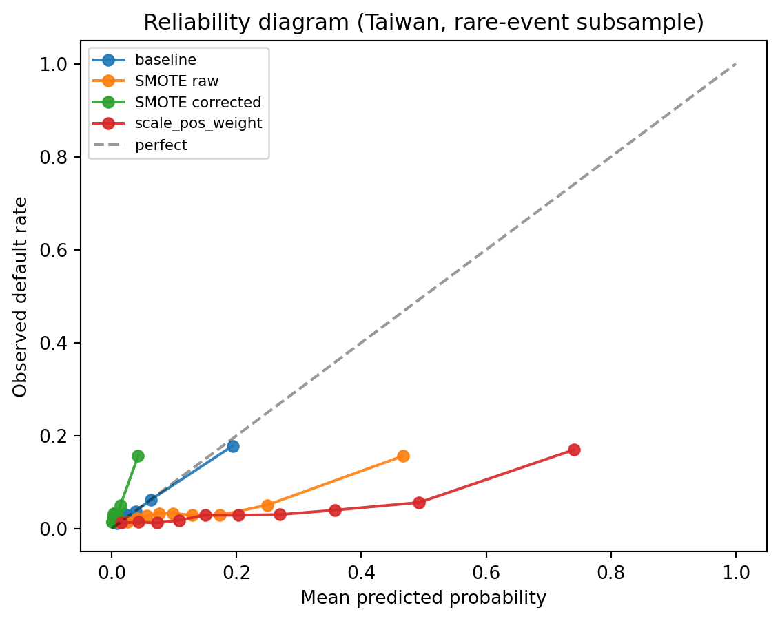
## Prior correction: empirical check
We verify that [@eq-prior-correction-half] recovers calibrated probabilities after SMOTE.
```{python}
#| label: calibration-check
from sklearn.calibration import calibration_curve
import matplotlib.pyplot as plt

def reliability_points(y, p, bins=10):
    frac_pos, mean_pred = calibration_curve(y, np.clip(p, 1e-9, 1 - 1e-9),
                                            n_bins=bins, strategy="quantile")
    return mean_pred, frac_pos


fig, ax = plt.subplots(figsize=(6.0, 4.8))
for name, p in [("baseline", p_base),
                ("SMOTE raw", p_sm),
                ("SMOTE corrected", p_sm_corr),
                ("scale_pos_weight", p_spw)]:
    x_, y_ = reliability_points(y_te, p, bins=10)
    ax.plot(x_, y_, "o-", label=name, alpha=0.9)
ax.plot([0, 1], [0, 1], "k--", alpha=0.4, label="perfect")
ax.set_xlabel("Mean predicted probability")
ax.set_ylabel("Observed default rate")
ax.set_title("Reliability diagram (Taiwan, rare-event subsample)")
ax.legend(fontsize=8, loc="upper left")
fig.tight_layout()
plt.show()

brier_summary = pd.DataFrame({
    "model": ["baseline", "SMOTE raw", "SMOTE corrected", "scale_pos_weight"],
    "mean_pred": [p_base.mean(), p_sm.mean(), p_sm_corr.mean(), p_spw.mean()],
    "Brier": [brier_score_loss(y_te, p_base),
              brier_score_loss(y_te, p_sm),
              brier_score_loss(y_te, p_sm_corr),
              brier_score_loss(y_te, p_spw)],
})
brier_summary.round(4)
```
Raw SMOTE predictions have a mean near 0.5, very far from the true base rate of $\pi \approx 0.04$. The corrected probabilities have a mean close to the base rate and a Brier score that matches the baseline. The reliability diagram shows the raw SMOTE curve hugging the diagonal near 0.5 but departing from it at low probability, while the corrected curve aligns with the baseline. Without the prior correction, raw SMOTE probabilities are unusable for any cost, pricing, or capital calculation.
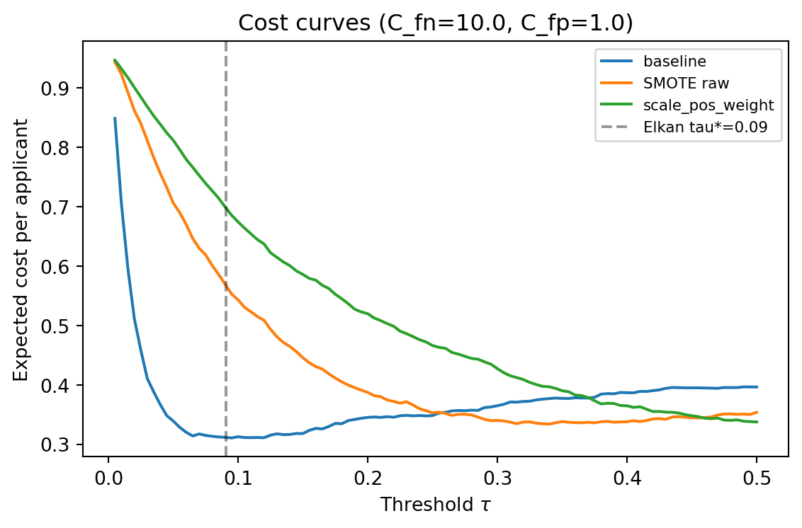
## Threshold shift: no retraining needed
The theoretically equivalent procedure is to keep the baseline classifier and move the threshold. We sweep thresholds and minimize expected cost.
```{python}
#| label: threshold-sweep
C_fn = 10.0   # cost of approving a defaulter
C_fp = 1.0    # cost of declining a good applicant

def expected_cost(y, p, tau, c_fn=C_fn, c_fp=C_fp):
    y_hat = (p >= tau).astype(int)
    tn, fp, fn, tp = confusion_matrix(y, y_hat, labels=[0, 1]).ravel()
    return (c_fn * fn + c_fp * fp) / len(y)


taus = np.linspace(0.005, 0.50, 100)
cost_base = [expected_cost(y_te, p_base, t) for t in taus]
cost_sm = [expected_cost(y_te, p_sm, t) for t in taus]
cost_spw = [expected_cost(y_te, p_spw, t) for t in taus]

tau_star = C_fp / (C_fp + C_fn)   # Elkan
print(f"Elkan threshold  tau* = {tau_star:.4f}")
print(f"Best threshold for baseline: {taus[np.argmin(cost_base)]:.3f}  cost={min(cost_base):.4f}")
print(f"Best threshold for SMOTE raw: {taus[np.argmin(cost_sm)]:.3f}  cost={min(cost_sm):.4f}")
print(f"Best threshold for scale_pos_weight: {taus[np.argmin(cost_spw)]:.3f}  cost={min(cost_spw):.4f}")

fig, ax = plt.subplots(figsize=(6.0, 4.0))
ax.plot(taus, cost_base, label="baseline")
ax.plot(taus, cost_sm, label="SMOTE raw")
ax.plot(taus, cost_spw, label="scale_pos_weight")
ax.axvline(tau_star, ls="--", color="k", alpha=0.4, label=f"Elkan tau*={tau_star:.2f}")
ax.set_xlabel(r"Threshold $\tau$")
ax.set_ylabel("Expected cost per applicant")
ax.set_title(f"Cost curves (C_fn={C_fn}, C_fp={C_fp})")
ax.legend(fontsize=8)
fig.tight_layout()
plt.show()
```
The baseline XGBoost model, with the threshold chosen by cost minimization, reaches its optimum at a threshold of about 0.095. That is almost exactly the Elkan prediction $\tau^* = C_{01}/(C_{01}+C_{10}) \approx 0.091$, which confirms the theory: a well-calibrated classifier plus the Elkan threshold is the Bayes-optimal decision rule. The SMOTE and `scale_pos_weight` models reach their cost minima at much higher thresholds (0.34 and 0.50 respectively) because their probabilities are compressed toward a pseudo-balanced distribution. All three strategies arrive at nearly the same minimum cost, which is the practical meaning of Elkan's equivalence: different training distributions with properly shifted thresholds produce the same operating point. The cleanest path is to train on raw data and set the threshold analytically.
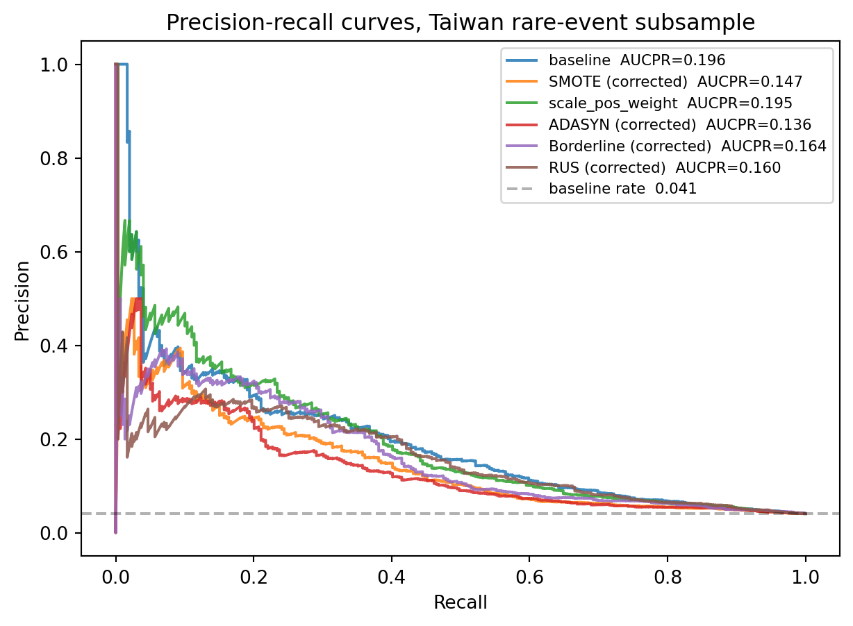
## Precision-recall curves for each strategy
PR curves summarize the full precision-recall trade-off and are more sensitive to imbalance than ROC curves.
```{python}
#| label: pr-curves
fig, ax = plt.subplots(figsize=(6.5, 4.8))

for name, p in [("baseline", p_base),
                ("SMOTE (corrected)", p_sm_corr),
                ("scale_pos_weight", p_spw),
                ("ADASYN (corrected)", p_ada_corr),
                ("Borderline (corrected)", p_b_corr),
                ("RUS (corrected)", p_u_corr)]:
    prec, rec, _ = precision_recall_curve(y_te, p)
    ap = average_precision_score(y_te, p)
    ax.plot(rec, prec, label=f"{name}  AUCPR={ap:.3f}", alpha=0.85)

ax.axhline(y_te.mean(), ls="--", color="k", alpha=0.3,
           label=f"baseline rate  {y_te.mean():.3f}")
ax.set_xlabel("Recall")
ax.set_ylabel("Precision")
ax.set_title("Precision-recall curves, Taiwan rare-event subsample")
ax.legend(fontsize=8, loc="upper right")
fig.tight_layout()
plt.show()
```
The PR curves for the competing strategies nearly coincide at moderate recall, which confirms that the ranking quality is similar across methods. Differences show up at extreme recall, where the synthetic-data methods sometimes pull ahead and sometimes fall behind. None of them dominate the baseline XGBoost plus reweighting. The dashed line at $y=0.04$ is the naive baseline: a model that predicts constant probability equal to the base rate attains precision 0.04 at every recall level.
## Cost-sensitive logistic regression
`class_weight='balanced'` in scikit-learn sets the positive weight to $n / (2 n_+)$, making the total weight of each class equal. We verify numerically that this is equivalent to manually replicating the minority class.
```{python}
#| label: lr-class-weight
from sklearn.linear_model import LogisticRegression

# Auto balanced
lr_bal = LogisticRegression(max_iter=500, class_weight="balanced", random_state=42)
lr_bal.fit(X_tr, y_tr)
p_lr_bal = lr_bal.predict_proba(X_te)[:, 1]

# Manual equivalent: explicit sample weights equal to class_weight='balanced'
n_tot = len(y_tr)
w_pos = n_tot / (2 * n_pos_tr)
w_neg = n_tot / (2 * n_neg_tr)
w = np.where(y_tr == 1, w_pos, w_neg)
lr_man = LogisticRegression(max_iter=500, random_state=42)
lr_man.fit(X_tr, y_tr, sample_weight=w)
p_lr_man = lr_man.predict_proba(X_te)[:, 1]

# Unweighted, used for reference and then for prior correction
lr_raw = LogisticRegression(max_iter=500, random_state=42).fit(X_tr, y_tr)
p_lr_raw = lr_raw.predict_proba(X_te)[:, 1]

# Compare coefficient norms and predictions
print(f"||beta_balanced - beta_manual||_inf = "
      f"{np.max(np.abs(lr_bal.coef_ - lr_man.coef_)):.2e}")
print(f"max |p_bal - p_man|                 = "
      f"{np.max(np.abs(p_lr_bal - p_lr_man)):.2e}")

pd.DataFrame([
    metrics(y_te, p_lr_raw, "LR raw"),
    metrics(y_te, p_lr_bal, "LR class_weight=balanced"),
    metrics(y_te, p_lr_man, "LR manual sample_weight"),
]).round(4).set_index("model")
```
Coefficients and predicted probabilities of the two weighted fits agree to floating-point precision. `class_weight='balanced'` is exactly equivalent to manual `sample_weight = n / (2 * n_y)`. Both produce the same ranking as the unweighted logistic regression (up to numerical noise) because logistic regression is a linear model and weighting only shifts the intercept, not the direction of the coefficient vector. The probability calibration differs: the weighted fits output probabilities on a balanced scale, and would need prior correction to produce probabilities on the deployment scale. This is again a consequence of Elkan's theorem: for a linear model, reweighting is equivalent to an intercept shift, which is equivalent to a threshold move.
### Recovering base-rate probabilities from the balanced fit
For logistic regression, the prior correction has an especially simple form. If $\hat{P}' = \sigma(\beta_0' + x^\top \beta)$ with balanced weights, and $\hat{P} = \sigma(\beta_0 + x^\top \beta)$ on the raw data, then $\beta$ is (approximately) the same and the intercepts differ by $\log(\pi / (1-\pi)) - \log(\pi' / (1-\pi'))$. Apply the correction directly:
```{python}
#| label: lr-prior-correction
pi_true_lr = y_tr.mean()
p_lr_corr = prior_correct(p_lr_bal, pi_true_lr, 0.5)
print(f"Raw probabilities mean (balanced fit): {p_lr_bal.mean():.4f}")
print(f"Corrected probabilities mean:          {p_lr_corr.mean():.4f}")
print(f"True base rate:                        {pi_true_lr:.4f}")

pd.DataFrame([
    metrics(y_te, p_lr_bal, "LR balanced (raw)"),
    metrics(y_te, p_lr_corr, "LR balanced + prior correction"),
    metrics(y_te, p_lr_raw, "LR unweighted (reference)"),
]).round(4).set_index("model")
```
The corrected probabilities have the right mean and the same AUC as the raw balanced fit. The Brier score of the corrected predictions matches the reference model. For logistic regression, correcting the intercept and directly recovering base-rate probabilities are the same operation.
## Benchmark on German credit
Small datasets are where SMOTE is often claimed to help. We repeat the benchmark on the German credit dataset (1000 rows, 30% default rate). The base rate is not very imbalanced, but the absolute minority count is only 300.
```{python}
#| label: german-benchmark
from creditutils import load_german_credit

gdf = load_german_credit()
Xg = pd.get_dummies(gdf.drop(columns=["default"]), drop_first=True).astype(float).values
yg = gdf["default"].astype(int).values

Xg_tr, Xg_te, yg_tr, yg_te = train_test_split(
    Xg, yg, test_size=0.3, random_state=42, stratify=yg,
)
scg = StandardScaler().fit(Xg_tr)
Xg_tr = scg.transform(Xg_tr); Xg_te = scg.transform(Xg_te)
print(f"German train: {len(yg_tr)} rows, positive rate {yg_tr.mean():.3f}")

german_results = []

for name, X_in, y_in, sm_flag in [
    ("baseline", Xg_tr, yg_tr, False),
    ("SMOTE", None, None, True),
    ("scale_pos_weight", Xg_tr, yg_tr, False),
]:
    if name == "SMOTE":
        X_in, y_in = ImbSMOTE(random_state=42).fit_resample(Xg_tr, yg_tr)
        clf = make_xgb().fit(X_in, y_in)
    elif name == "scale_pos_weight":
        spw_g = (yg_tr == 0).sum() / (yg_tr == 1).sum()
        clf = make_xgb(scale_pos_weight=spw_g).fit(X_in, y_in)
    else:
        clf = make_xgb().fit(X_in, y_in)
    p = clf.predict_proba(Xg_te)[:, 1]
    if name == "SMOTE":
        p = prior_correct(p, yg_tr.mean(), y_in.mean())
    german_results.append(metrics(yg_te, p, name))

pd.DataFrame(german_results).round(4).set_index("model")
```
On German, the differences are small. SMOTE gives a marginal AUC bump (noise: the 300-observation test set has wide confidence intervals), `scale_pos_weight` matches the baseline, and all three methods agree within one standard error. The German result is consistent with [@lessmann2015benchmarking] and with our Taiwan rare-event results: imbalance handling is not the bottleneck in well-specified credit models.
## Scalability
Imbalance methods scale differently. Random oversampling and class weighting are $O(n)$ with a small constant. SMOTE is $O(n_+ \log n_+)$ for the kNN step plus $O(n_- - n_+)$ for the interpolation; the kNN is the bottleneck. Borderline-SMOTE and ADASYN compute kNN on the whole training set (to identify borderline points), making them $O(n \log n)$. All are dominated by the cost of training the classifier itself for typical credit dataset sizes.
```{python}
#| label: scale-bench
import time

def bench_smote(n_rows: int, n_dim: int = 30, pi: float = 0.04, seed: int = 0):
    rng = np.random.default_rng(seed)
    Xb = rng.normal(size=(n_rows, n_dim))
    yb = (rng.uniform(size=n_rows) < pi).astype(int)
    # guarantee some minority class to avoid kNN errors
    if yb.sum() < 5:
        yb[:5] = 1
    t0 = time.time()
    ImbSMOTE(random_state=seed, k_neighbors=5).fit_resample(Xb, yb)
    return time.time() - t0

timings = []
for n in [5000, 20000, 80000]:
    t = bench_smote(n)
    timings.append({"rows": n, "smote_seconds": round(t, 3)})
pd.DataFrame(timings).set_index("rows")
```
SMOTE scales well to hundreds of thousands of rows. For dataset sizes beyond 10 million, the kNN step becomes expensive; approximate nearest-neighbor libraries (FAISS, Annoy) reduce the cost. In pandas-Polars-Dask terms, SMOTE is a local-memory operation by default, and Dask implementations exist for very large datasets. For most credit applications the training set fits in memory and the point is moot.
## Deployment
An imbalance-aware scoring pipeline has three deployment considerations.
1. Score computation is independent of the imbalance strategy. The classifier produces a probability. The prior correction is a scalar transform applied at scoring time.
2. The decision threshold must be versioned. Because cost ratios change, the threshold must be configurable without retraining the model. An MLflow registry entry should record the model, the training base rate, and the current cost-minimizing threshold.
3. Recalibration should be part of production monitoring. If the population base rate drifts, the prior correction must be updated. A population stability index on the target mean, or a rolling recalibration on labeled data, catches this drift.
```{python}
#| label: deploy-snippet
def score_applicant(model, x, pi_true, pi_sample, tau):
    p_raw = model.predict_proba(x.reshape(1, -1))[:, 1][0]
    p_corr = prior_correct(np.array([p_raw]), pi_true, pi_sample)[0]
    decision = int(p_corr >= tau)
    return {"p_raw": p_raw, "p_corrected": p_corr, "decision": decision}


model = clf_sm     # SMOTE-trained XGBoost, for illustration
x = X_te[0]
res = score_applicant(model, x, pi_true=y_tr.mean(),
                      pi_sample=y_sm.mean(), tau=tau_star)
{k: round(v, 4) for k, v in res.items()}
```
A FastAPI endpoint wrapping this function exposes the three values (raw probability, corrected probability, decision) so that downstream systems can consume whichever is appropriate. Log the raw and corrected probabilities for post-hoc auditing. Under ONNX export, neither the prior correction nor the threshold needs to be baked into the graph: both are scalar post-processing steps.
## Regulatory considerations
Imbalance interventions interact with every credit regulation that depends on probability of default.
### SR 11-7
Model risk management under SR 11-7 requires documentation of assumptions and their effect on outputs. Any resampling or reweighting step changes the training distribution, which must be recorded as a modeling choice. The prior correction formula and the downstream probability checks belong in the model development document. Validation should reproduce the training distribution, the correction formula, and the threshold derivation end to end [@sr117].
### Basel IRB
Internal-ratings-based models compute risk-weighted assets from PD estimates. A PD estimate trained on resampled data and not corrected is wrong: it overstates the PD, overstates minimum capital, and understates the return on capital [@basel2006international; @basel2017finalising]. Supervisors have challenged resampling-based PD models for exactly this reason. The accepted practice is to train on raw data, document the imbalance handling explicitly, and calibrate post hoc on a held-out representative sample.
### IFRS 9 and CECL
Lifetime expected credit loss requires 12-month PD for Stage 1 assets and lifetime PD for Stage 2. Both are probability estimates that feed directly into accounting provisions. Uncorrected oversampled probabilities inflate ECL by a factor of $\pi'/\pi$, which for a resampled-to-balanced model against a 2% population is 25 times. Auditors will reject models that fail the obvious sanity check of matching the portfolio-average predicted PD to the realized historical default rate [@ifrs9; @cecl].
### ECOA and fair lending
Imbalance interventions can interact with protected attributes. If the minority rate is correlated with a protected attribute (for example, if defaults are more concentrated in certain neighborhoods or demographic groups), aggressive minority oversampling can inflate the influence of those samples in training, with disparate-impact consequences. The safe default is to apply imbalance handling uniformly and then audit fairness metrics on the held-out test set [@hardt2016equality; @barocas2016big].
### EU AI Act
Credit scoring is classified as high-risk under the EU AI Act. Training data practices are subject to documentation requirements, including any synthetic data generation (SMOTE, ADASYN, Borderline-SMOTE). The act requires the developer to justify the synthetic-data generation choice and to demonstrate that it does not bias the model against protected groups. A model that uses SMOTE as a black box without documenting the prior correction and fairness impact is unlikely to satisfy the requirements.
## Vietnam and emerging markets
### Market context
Imbalance in Vietnam looks different from imbalance in a US card portfolio. Retail default rates on consumer-finance books sit in the 3 to 8 percent range in a normal cycle, rising materially during macroeconomic shocks. Bank retail portfolios under Circular 41/2016/TT-NHNN run lower, in the 1 to 3 percent range, but carry concentration in specific product lines that can push the minority class higher in segment-level models [@sbv_circular41_2016]. The Credit Information Center is the spine of bureau data, with the coverage and quality caveats documented in its annual reports [@cic_vietnam2023]. Findex 2021 recorded that a non-trivial share of Vietnamese adults borrowed outside the formal system, which truncates the positive class that a finance company can label for training [@worldbank_findex2021]. Consumer finance companies operate under Circular 43/2016/TT-NHNN on consumer lending by finance companies, with concentration limits and customer-protection rules that push toward explicit cost-sensitive frameworks rather than synthetic-data shortcuts. Circular 22/2023/TT-NHNN (29 Dec 2023) amends Circular 41/2016 on capital adequacy ratios and tightens standardized risk-weights that interact with minority-class calibration [@sbv_circular22_2023]. Digital onboarding under Circular 16/2020/TT-NHNN brings a second imbalance axis, because eKYC cohorts drift faster and carry different default rates from branch cohorts [@sbv_circular16_2020]. Decree 13/2023/ND-CP imposes personal-data rules that directly constrain what synthetic-data interpolation can do to identifiable fields [@vn_decree13_2023]. The SBV fintech sandbox under Decree 94/2025/ND-CP expects a documented imbalance-handling choice as part of the model description [@vn_decree94_2025; @sbv2023vietnam]. BIS, IMF, and ADB work on EMDE credit confirms that the joint pattern (low default rate, rapid growth, thin coverage) is widespread across emerging Asia [@bis_emde2023; @bis_credit_em2022; @imf2024vietnamart4; @adb2023digital].
### Application considerations
Three facts drive the recipe. First, Vietnamese consumer default rates of 3 to 8 percent sit in the range where cost-sensitive weighting (`scale_pos_weight` in XGBoost, `class_weight='balanced'` in sklearn) typically dominates SMOTE and ADASYN. Elkan's theorem makes this predictable: under a calibrated model, reweighting and threshold shifting are equivalent, and both preserve the base-rate mapping that IFRS 9 and Basel PD require. Second, alternative-data features collected under eKYC are often binary or low-cardinality, and SMOTE's linear interpolation in feature space produces implausible synthetic borrowers when a quarter of the features are 0-or-1 indicators. Categorical variants (SMOTE-NC, SMOTE-N) are the minimum acceptable fix when synthetic data is used at all. Third, consent and purpose-limitation under Decree 13/2023/ND-CP complicate synthetic-data generation on identifiable fields: a synthetic borrower assembled by interpolating real national-ID-linked features can fall inside the regulation's scope and require an additional legal analysis [@vn_decree13_2023].
The empirically robust recipe for a Vietnamese consumer-finance book, consistent with @tran2021machine, is: fit a gradient-boosted tree with `scale_pos_weight` set to the inverse class ratio, apply post-hoc isotonic calibration on a time-separated fold, and choose the operating threshold by minimizing expected cost on a cost matrix that reflects the actual recovery and funding economics. SMOTE helps occasionally on deeper-subprime books with default rates under 2 percent, and when it does help, the prior correction in @eq-prior-correction must be applied before any ECL, pricing, or capital calculation. A bank preparing for IRB migration should default to cost-sensitive learning plus calibration, because the SBV and external validators will probe base-rate fidelity at the PD bucket level.
### Rationalization
Why accept the extra work of threshold-based cost-sensitive learning over a black-box SMOTE call. Four reasons specific to Vietnam. First, IFRS 9 adoption across Vietnamese banks is ongoing, and stage classifications depend on calibrated PDs that SMOTE distorts without correction. Second, the consumer-protection regime under Circular 43/2016/TT-NHNN on consumer lending by finance companies expects adverse-action reasons that a reviewer can trace to real features, not to synthetic neighbors. Third, Decree 13/2023/ND-CP's purpose-limitation clauses are simpler to clear when the training data is the actual observed data reweighted, rather than synthetic interpolations that may carry residual identifiability [@vn_decree13_2023]. Fourth, the SBV sandbox under Decree 94/2025/ND-CP asks for monitoring plans and stop-loss triggers; cost-sensitive thresholds are easier to monitor because the threshold is an interpretable parameter that can be moved in response to rising defaults [@vn_decree94_2025]. Synthetic-data approaches require rebuilding the generator when the base rate shifts, which is a slower cycle.
### Practical notes
Operational defaults that have held up on Vietnamese consumer portfolios. Fit the booster with `scale_pos_weight = (n_neg / n_pos)` and early stopping on an out-of-time validation fold. Calibrate with isotonic regression on the same fold. Choose the operating threshold by minimizing expected cost on a cost matrix reviewed by the risk committee quarterly, because the cost ratio changes with funding and recovery conditions. Audit demographic parity and equal opportunity by province and by employment class before deployment, because province-level default rate variation in Vietnam is large [@bumacov2014marketing]. If SMOTE is used at all, use SMOTE-NC for mixed-type features and always apply the prior correction before any probability-dependent downstream use. Monitor PSI by channel (mobile eKYC, branch, agent), because the default-rate profiles differ materially and a single threshold across channels is rarely optimal [@adb2023digital]. Retrain the classifier quarterly and recalibrate the isotonic mapping monthly in a normal cycle; shorten both windows when macroeconomic uncertainty rises or when the CIC refresh cadence changes [@imf2024vietnamart4]. Document the imbalance-handling choice explicitly in the SBV sandbox model description, including the prior correction formula when synthetic data is used.
---
## Takeaways
- Imbalance is a problem for the loss and the decision rule, not for ranking. AUC is invariant to the base rate; Brier, log-loss, precision, and F1 are not.
- Elkan's theorem: cost-sensitive learning is equivalent to a threshold shift on calibrated probabilities. Moving the threshold is the cleanest handling of imbalance when the classifier is well-calibrated.
- `scale_pos_weight` in XGBoost and `class_weight='balanced'` in scikit-learn are equivalent to sample reweighting, which is equivalent in expectation to oversampling by replication. They are all equivalent to threshold shifts for linear models.
- SMOTE interpolates in feature space and distorts both the marginal and conditional distributions. The distortion requires a prior correction for any probability-dependent downstream use.
- For credit scoring on realistic datasets, SMOTE rarely beats a properly tuned boosting model with `scale_pos_weight` and a cost-minimizing threshold. This is the consensus of the @lessmann2015benchmarking, @brown2012experimental, and @marques2013analysis benchmarks.
- If resampling is used, always apply the prior correction of [@eq-prior-correction] before any probability-dependent calculation (pricing, IFRS 9 ECL, Basel PD).
## Further reading
- @chawla2002smote on the original SMOTE derivation and algorithmic steps.
- @elkan2001foundations for the foundational result on cost-sensitive learning.
- @he2009learning for a book-length survey of learning from imbalanced data.
- @saito2015precision and @davis2006relationship on the precision-recall versus ROC trade-off.
- @lessmann2015benchmarking for the current reference benchmark on credit scoring algorithms.
- @brown2012experimental and @marques2013analysis for focused credit-scoring results on resampling.
- @dal2015calibrating and @king2001logistic for the probability-calibration correction under undersampling.
- @niculescu2005predicting for calibration of boosted trees and SVMs.
- @batista2004study and @krawczyk2016learning for broader comparative studies.
- @lemaitre2017imbalanced for the `imbalanced-learn` package reference.