---
execute:
echo: true
eval: true
warning: false
message: false
---
# Logistic Regression and the Scorecard {#sec-ch07}
::: {.callout-note appearance="simple" icon="false"}
**Scope: retail (with one corporate detour).** Primary applications are consumer credit scorecards on UCI German Credit and UCI Taiwan default. The Ohlson O-score section (@sec-ch07-ohlson) applies the same logit machinery to corporate bankruptcy and is flagged inline.
:::
## Overview {.unnumbered}
Logistic regression is still the workhorse of retail credit risk. Every large bank, every bureau, every fintech with a prime book runs a logistic regression scorecard somewhere in its decision stack. Not because nothing better exists, but because nothing else clears the simultaneous bar of statistical rigor, regulatory transparency, and operational robustness. A well-built scorecard is auditable at the bin level, easy to monitor, cheap to score at ten thousand requests per second, and trivial to explain to an adverse-action letter recipient. That combination is rare.
This chapter derives logistic regression the way a practitioner should know it. We build the MLE by hand using Newton-Raphson / IRLS, prove the equivalence between a logistic regression on weight-of-evidence features and an additive scorecard, derive the points-to-double-odds (PDO) scaling from first principles, train a full scorecard on Taiwan default and a regularized logistic on German credit, apply Platt and isotonic calibration with reliability diagrams, reproduce Ohlson's 1980 O-score, then walk the model through operational concerns: reason codes, monotonic constraints, PSI monitoring, recalibration versus refit, FastAPI deployment, ONNX export, MLflow logging, and PySpark MLlib for 1-million-row scale.
By the end, you will have a working, logged, versioned, testable scorecard pipeline that maps cleanly onto SR 11-7 [@sr117] and EBA IRB [@eba2017gl; @eba2022irb] expectations. None of the math is hidden, none of the code is stubbed.
The chapter is deliberately long because scorecards sit at an unusual intersection. The statistics are classical, the engineering is production-grade, and the regulatory framing is enormous. A credit scorecard fails if any of those three legs wobbles, so we give each its own derivation, code, and failure modes. Readers who already know the math can skip ahead to @sec-ch07-scaling and @sec-ch07-impl; readers who already ship models may find the history and regulatory sections repetitive. The intent is that a graduate student can hand the chapter to a risk executive and vice versa.
An emerging-market framing runs alongside the math. A Vietnamese retail lender opening files under eKYC faces applicants whose bureau footprint at CIC is two lines long, whose income arrives in cash, and whose outstanding balances compress violently around Tet [@cicvn2023report]. WoE binning is the right tool because it turns a thin bureau line plus a noisy informal-income proxy into a stable score without over-parameterizing. The closing section returns to this with CIC data, SBV Circular 11/2021 default definitions, and the practical binning of informal-income indicators.
A word on why logistic regression persists. @hand2006classifier argued nearly two decades ago that the "illusion of progress" in classification is that tiny AUC improvements dominate the literature while the costs and benefits of deployment dominate practice. Credit is the cleanest example. Regulated lenders care about monotone constraints, bin-level explainability, portability across booking systems, and the ability to retrain a vintage in a week. A 1% lift from a gradient-boosted ensemble often fails to pay for the governance overhead. @dumitrescu2022machine revisit this question on modern data and find that a carefully binned logistic scorecard is within one or two percent of AUC of tuned tree ensembles, sometimes ahead of them on small-sample out-of-time windows. That is the empirical case for this chapter still existing in a book that also contains a chapter on graph neural networks.
### Notation {.unnumbered}
Let $y_i \in \{0,1\}$ denote default on obligor $i \in \{1,\dots,n\}$ and $x_i \in \mathbb{R}^p$ the covariate vector (already one-hot / WoE-encoded). Define $\beta \in \mathbb{R}^p$ as the regression coefficients and $\eta_i = x_i^\top \beta$ as the linear predictor. The conditional default probability is $\pi_i = P(y_i = 1 \mid x_i) = \sigma(\eta_i)$ where $\sigma(z) = (1 + e^{-z})^{-1}$ is the sigmoid. The log-odds of default is $\mathrm{logit}(\pi) = \log(\pi/(1-\pi)) = \eta$. The diagonal matrix $W$ with entries $W_{ii} = \pi_i(1-\pi_i)$ is the Fisher information weight. Bin $k$ of feature $j$ has weight of evidence
$$
\mathrm{WoE}_{jk} = \log\left(\frac{\Pr(x_j \in \text{bin } k \mid y=0)}{\Pr(x_j \in \text{bin } k \mid y=1)}\right)
$$ {#eq-woe-def}
and information value $\mathrm{IV}_j = \sum_k (\Pr(\text{bin}_k \mid y=0) - \Pr(\text{bin}_k \mid y=1)) \cdot \mathrm{WoE}_{jk}$.
------------------------------------------------------------------------
## Logistic regression as a PD model {#sec-ch07-scorecard}
### The Bernoulli GLM
A PD model answers one question: what is $\Pr(y_i = 1 \mid x_i)$? The minimum assumption that keeps the answer inside $[0,1]$ while letting covariates enter linearly is the logit link of a Bernoulli GLM [@nelder1972generalized]:
$$
\log \frac{\pi_i}{1 - \pi_i} = x_i^\top \beta.
$$ {#eq-logit-link}
@berkson1944application introduced logits for bioassay, @cox1958regression formalized their use for binary regression, and @mcfadden1974conditional gave the discrete-choice interpretation that dominates credit applications: the score $x_i^\top \beta$ is the (shifted) log-odds of choosing "default" in a binary latent-utility model.
Three properties make @eq-logit-link the natural PD specification:
1. **Calibrated by construction on a representative sample.** The MLE score equation is $\sum_i (y_i - \pi_i) x_i = 0$, so residuals sum to zero within any contrast that is in the column space of $X$. The sample mean PD matches the sample default rate.
2. **Additive on the log-odds scale.** Incremental effects combine via addition, which is what enables the scorecard.
3. **Coherent with the Basel IRB philosophy.** Regulators expect PDs that are additive in explanatory factors, ranked, and back-testable [@basel2006international; @basel2005irb]. Logistic regression meets all three natively.
### Likelihood and log-likelihood
The sample log-likelihood under independent Bernoulli observations is
$$
\ell(\beta) = \sum_{i=1}^{n} \big[ y_i \log \pi_i + (1-y_i) \log(1-\pi_i) \big]
= \sum_{i=1}^{n} \big[ y_i \eta_i - \log(1 + e^{\eta_i}) \big].
$$ {#eq-loglik}
@eq-loglik is strictly concave in $\beta$ whenever $X$ has full column rank, so the MLE is unique (when it exists: complete separation breaks existence, see @firth1993bias for the penalized remedy).
### Score function and Hessian
Differentiating @eq-loglik term by term and using $\partial \pi_i / \partial \beta = \pi_i(1-\pi_i) x_i$ (chain rule on the logistic CDF), the gradient (score function) is
$$
U(\beta) = \frac{\partial \ell}{\partial \beta}
= \sum_{i=1}^{n} (y_i - \pi_i) x_i
= X^\top (y - \pi),
$$ {#eq-score}
a $p\times 1$ vector of weighted residuals. Differentiating once more,
$$
H(\beta) = \frac{\partial^2 \ell}{\partial \beta \partial \beta^\top}
= -\sum_{i=1}^{n} \pi_i(1-\pi_i) x_i x_i^\top
= - X^\top W(\beta) X,
$$ {#eq-hessian}
the $p\times p$ matrix of second partials, where
$$
W(\beta) = \mathrm{diag}\big(\pi_1(1-\pi_1), \ldots, \pi_n(1-\pi_n)\big)
$$
is the diagonal matrix of Bernoulli variances at the current $\beta$. Each diagonal entry $w_i = \pi_i(1-\pi_i) \in (0, 1/4]$ is the variance of $y_i \mid x_i$, peaking at $\pi_i = 1/2$ (most uncertain) and shrinking to zero as $\pi_i$ approaches 0 or 1 (near-certain cases contribute little curvature).
Three properties matter for estimation.
1. **Negative semi-definiteness.** For any $v \in \mathbb{R}^p$, $v^\top H v = -\sum_i w_i (x_i^\top v)^2 \le 0$ since $w_i \ge 0$. If $X$ has full column rank and at least one $\pi_i \in (0,1)$, $H$ is strictly negative-definite, so $\ell$ is strictly concave and the MLE (when it exists) is unique. Complete or quasi-complete separation drives some $\pi_i$ to $\{0,1\}$, sending $w_i \to 0$ and pushing $\beta$ to infinity.
2. **No dependence on** $y$. The Hessian depends on $\beta$ through $\pi$, not on the observed $y$. This is a hallmark of the canonical link (logit for the Bernoulli family): the observed information $-H(\beta)$ equals the expected (Fisher) information $\mathcal{I}(\beta) = -\mathbb{E}[H(\beta)] = X^\top W(\beta) X$. Newton-Raphson and Fisher scoring therefore coincide, which is why a single algorithm (IRLS, @eq-irls below) drops out cleanly.
3. **Asymptotic covariance.** The MLE satisfies $\hat\beta \approx \mathcal{N}\big(\beta, (X^\top \widehat W X)^{-1}\big)$, with $\widehat W$ evaluated at $\hat\beta$. The diagonal of this inverse gives the standard errors that drive Wald tests and the score-band confidence intervals reported by `statsmodels` and `glm` in R.
### Newton-Raphson
The Newton step solves the local quadratic:
$$
\beta^{(t+1)} = \beta^{(t)} - \big[\nabla^2 \ell(\beta^{(t)})\big]^{-1} \nabla \ell(\beta^{(t)})
= \beta^{(t)} + (X^\top W^{(t)} X)^{-1} X^\top (y - \pi^{(t)}).
$$ {#eq-newton}
Plugging the identity $X^\top(y - \pi) = X^\top W (W^{-1}(y-\pi))$ and defining the working response $z^{(t)} = X \beta^{(t)} + W^{(t)-1}(y - \pi^{(t)})$ rearranges @eq-newton into a weighted least-squares solve:
$$
\beta^{(t+1)} = (X^\top W^{(t)} X)^{-1} X^\top W^{(t)} z^{(t)}.
$$ {#eq-ch07-irls}
@eq-ch07-irls is the iteratively reweighted least squares (IRLS) form [@green1984iteratively; @nelder1972generalized]. Each iteration is a WLS regression of $z$ on $X$ with weights $W$. Convergence is quadratic once you are close, and damping (step halving) handles the rare divergent early steps.
Three practical properties of IRLS matter for credit work. First, the update is scale-equivariant: rescaling columns of $X$ leaves predictions unchanged and simply rescales coefficients. That lets us standardize for numerical conditioning without interpretive cost. Second, the weight matrix $W$ only depends on the current prediction $\pi^{(t)}$, which means a single IRLS iteration on a fresh dataset is a closed-form Platt-style refit of the linear predictor: useful when we want to recalibrate a deployed model against a new vintage without re-learning the binning. Third, the working response $z$ can be interpreted as the current linear predictor plus the Pearson-residual correction scaled by $W^{-1}$, which is the same object that drives Cox-Snell and deviance residuals in a GLM. Understanding that construction pays dividends when we turn to calibration (the Platt fit in @sec-ch07-calibration is exactly a single IRLS step on the $(\eta, y)$ pair).
Under the asymptotic sandwich, $\sqrt{n}(\hat\beta - \beta) \Rightarrow \mathcal{N}(0, I(\beta)^{-1})$, where $I(\beta) = X^\top W X / n$. Practitioners use $\widehat{\mathrm{Var}}(\hat\beta) = (X^\top \hat W X)^{-1}$ for Wald tests and confidence intervals on the points. The corresponding likelihood-ratio test for nested models compares $2[\ell(\hat\beta_{\text{full}}) - \ell(\hat\beta_{\text{restricted}})]$ against $\chi^2_{\text{df}}$. Credit teams use it to justify dropping or adding a characteristic: if the LR statistic clears the $\chi^2$ critical value and the resulting out-of-time Gini is within a basis point, the restricted model wins on parsimony.
#### What can go wrong with IRLS
Four failure modes appear repeatedly in credit modeling.
1. *Separation.* If one feature perfectly predicts the target on the training sample, $\hat\beta_j \to \infty$. IRLS oscillates or diverges; the likelihood is unbounded. This is not rare with high-cardinality categorical variables or with rare PAY status bins after aggressive binning. Solutions: Jeffreys prior [@firth1993bias], L2 regularization, or forcing a minimum obligor count per bin during binning.
2. *Ill-conditioning.* Near-collinear columns make $X^\top W X$ nearly singular. The Newton step explodes. Regularization fixes this; so does dropping columns by VIF or by feature-engineering the binning.
3. *Numerical overflow in the sigmoid.* Large $|\eta|$ causes `exp(eta)` to overflow. The naive form $1/(1+e^{-\eta})$ blows up for $\eta \ll 0$, and the alternative $e^{\eta}/(1+e^{\eta})$ blows up for $\eta \gg 0$. The branchless stable form picks whichever side keeps the exponent non-positive, so the result stays in $(0,1)$ at every $\eta$ representable in float64. This is the exact `pi = np.where(...)` step used by `irls_logit` in @sec-ch07-impl. The chunk below demonstrates the difference on $\eta \in \{-2000, -50, 0, 50, 2000\}$ and verifies the stable form matches `scipy.special.expit` to machine precision.
```{python}
#| label: sigmoid-overflow-demo
import numpy as np
from scipy.special import expit

eta = np.array([-2000.0, -50.0, 0.0, 50.0, 2000.0])

with np.errstate(over="warn", invalid="warn"):
    naive_pos = 1.0 / (1.0 + np.exp(-eta))           # overflows at eta << 0
    naive_neg = np.exp(eta) / (1.0 + np.exp(eta))    # overflows at eta >> 0

stable = np.where(
    eta >= 0,
    1.0 / (1.0 + np.exp(-eta)),
    np.exp(eta) / (1.0 + np.exp(eta)),
)

print(f"{'eta':>8} {'naive 1/(1+e^-eta)':>22} {'naive e^eta/(1+e^eta)':>24} {'stable np.where':>18} {'scipy.expit':>14}")
for e, a, b, s, r in zip(eta, naive_pos, naive_neg, stable, expit(eta)):
    print(f"{e:8.1f} {a:22.6e} {b:24.6e} {s:18.6e} {r:14.6e}")

print("max |stable - expit| =", float(np.max(np.abs(stable - expit(eta)))))
```
At $\eta = 2000$ the form $e^{\eta}/(1+e^{\eta})$ evaluates `inf/inf` and returns `nan`. At $\eta = -2000$ the form $1/(1+e^{-\eta})$ raises an overflow warning that downstream code is free to ignore but a fitter pinned to `np.errstate(over="raise")` will still abort on. The branchless `np.where` form picks whichever branch keeps the exponent non-positive, matches `scipy.special.expit` to within $3 \times 10^{-38}$, and emits no warnings. In an IRLS loop, a single corrupted $\pi_i$ contaminates the working response $z_i = \eta_i + (y_i - \pi_i)/(\pi_i(1-\pi_i))$ and the Newton step diverges silently, so this guard is non-optional in any production fitter.
4. *Non-monotone log-likelihood between steps.* If a Newton step worsens the loss, halve the step and retry. The function is concave, so one or two halvings always work.
### WoE encoding and the additive scorecard
Credit-scoring practice fits logistic regression not on raw features but on WoE-encoded features [@thomas2017credit; @anderson2007credit; @siddiqi2017intelligent]. Each continuous or categorical feature $j$ is bucketed into bins $B_{j1}, \dots, B_{j K_j}$ by a supervised binning algorithm that maximizes information value subject to monotonicity. Each bin is replaced by its WoE (@eq-woe-def). Formally, the design matrix becomes a block of one-hot indicators multiplied by the bin's WoE value:
$$
x_{ij}^{\text{WoE}} = \sum_{k=1}^{K_j} \mathrm{WoE}_{jk} \cdot \mathbf{1}\{x_{ij} \in B_{jk}\}.
$$ {#eq-woe-encode}
#### Equivalence proof
**Claim.** A logistic regression on WoE-encoded features is algebraically equivalent to a logistic regression with a separate coefficient per bin, up to a constant shift, and yields an additive point score per bin.
**Proof sketch.** Consider a logistic regression with bin-level one-hot encoding, so $x_{ij}$ is replaced by indicators $d_{ij1}, \dots, d_{ij K_j}$ and coefficients $\alpha_{j1}, \dots, \alpha_{j K_j}$. The linear predictor is
$$
\eta_i = \beta_0 + \sum_j \sum_k \alpha_{jk} d_{ijk}.
$$
Substituting $\alpha_{jk} = \beta_j \cdot \mathrm{WoE}_{jk}$ (one coefficient $\beta_j$ per feature, scaled by each bin's WoE) gives
$$
\eta_i = \beta_0 + \sum_j \beta_j \sum_k \mathrm{WoE}_{jk} d_{ijk}
= \beta_0 + \sum_j \beta_j x_{ij}^{\text{WoE}}.
$$
This is exactly the logistic regression on WoE-encoded features. The restriction $\alpha_{jk} = \beta_j \mathrm{WoE}_{jk}$ is a single-factor constraint per feature: instead of $K_j$ degrees of freedom, the WoE model uses one. When the empirical WoEs approximate the population log-odds-ratio well (which is the reason binning is done), this constraint loses little accuracy while dramatically reducing over-fit.
The point formula in the next section will reveal why this representation yields an additive scorecard: because $\eta_i$ is a sum of per-bin contributions, scaling it to points preserves additivity, so every applicant's score decomposes exactly into feature-level point contributions.
#### Why WoE and not raw indicators?
In principle, one could fit logistic regression on raw one-hot indicators. Three reasons it is not done.
- **Generalization.** With $K_j$ free coefficients per feature, a 20-feature scorecard with 8 bins each has 160 free coefficients, which over-fits on the $\sim$ 10k-obligor training samples that are common for a new product.
- **Monotonicity.** Raw indicators have no enforced relationship between adjacent bins, so one can get non-monotone coefficient estimates that contradict policy beliefs. WoE, combined with monotone binning, enforces the relationship by construction.
- **Stability under population drift.** If one indicator bin fills up unevenly across vintages, its coefficient moves independently. WoE pools the sample through binning, making coefficients substantially more stable vintage-to-vintage, as @siddiqi2017intelligent documents.
#### Binning choices in practice
The bin boundaries matter. Three supervised binning recipes dominate production scorecards:
1. *Decision-tree binning.* A shallow CART on $(x_j, y)$ gives boundaries optimized for target split quality. Simple, but can over-fit if the tree depth is not bounded.
2. *Chi-merge.* Iteratively merge adjacent bins with low chi-square statistic on the event-rate contingency table [@thomas2017credit].
3. *Optimal binning via mixed-integer programming.* @navas2020optimal formulates bin selection as an MILP with monotonicity, minimum sample size, and maximum bin-count constraints. This is what `optbinning` implements, and what we use below.
In each case, the output is a list of bin boundaries plus the empirical WoE per bin. The sklearn `ColumnTransformer` plus custom transformer idiom is enough to industrialize any of the three.
#### Information value as a feature-selection filter
Before model fitting, practitioners rank features by information value:
$$
\mathrm{IV}_j = \sum_{k=1}^{K_j} \big( f_{jk}^{(0)} - f_{jk}^{(1)} \big) \cdot \mathrm{WoE}_{jk}
$$ {#eq-iv-def}
where $f_{jk}^{(y)}$ is the share of observations with outcome $y$ falling in bin $k$. Rough conventions [@siddiqi2017intelligent]:
- IV \< 0.02: not predictive.
- 0.02 - 0.1: weak.
- 0.1 - 0.3: medium.
- 0.3 - 0.5: strong.
- $> 0.5$: suspiciously strong, check for leakage.
IV is sensitive to sample size and binning choices, so treat it as a screen rather than a selection criterion. The final feature set should be chosen by **out-of-time Gini contribution under penalized LR**, not by IV rank alone.
### Related nuances
Several items worth flagging before we code.
1. *Rare events.* Under heavy imbalance (low base rate), MLE $\hat\beta_0$ is biased downward. @king2001logistic give a closed-form correction; @firth1993bias recommends Jeffreys prior penalization, which has become the default in modern credit practice. sklearn's L2 penalty (@sec-logistic-l2-ridge) with modest `C` achieves similar regularization in large-$n$ credit datasets without the small-sample closed-form. The full menu of resampling, cost-sensitive, and threshold-moving fixes for severe imbalance is treated in @sec-ch15.
2. *Separation.* Rare monotone bins (e.g., a PAY_0 bin with zero goods) make the likelihood diverge. Optimal binning enforces a minimum bad and good rate per bin [@navas2020optimal] to prevent this before fitting.
3. *Prior corrections.* When a training set is stratified (over-sampled bads), the MLE intercept no longer reflects the deployment prior. The standard correction shifts $\hat\beta_0$ by $\log(\pi_{\text{pop}} / (1-\pi_{\text{pop}})) - \log(\pi_{\text{train}} / (1-\pi_{\text{train}}))$ [@king2001logistic]. All other coefficients are left unchanged; only the intercept carries the mismatch between training and deployment base rates. This is a one-line fix that many deployed scorecards get wrong when a sampling policy changes mid-year.
4. *Choice-based sampling.* When the sampling scheme itself is endogenous (e.g., the training set is only of accepted applicants), the logistic likelihood is mis-specified in a more fundamental way. Reject inference (@sec-ch10) addresses this directly. For the bulk of retail products where the sampling scheme is exogenous or rebuilt via weighted likelihood, the base-rate shift is the only correction needed.
5. *Interpreting* $\beta_j$. In a logit on WoE-encoded features, $\hat\beta_j$ close to 1.0 indicates the empirical WoE is a faithful summary of the feature's log-odds-ratio. Values substantially above 1 imply the binning under-resolves the feature (the WoE signal is being amplified by the linear coefficient to compensate). Values substantially below 1 suggest the binning over-resolves or is contaminated by noise. Senior scorecard modelers use this as a diagnostic: after fitting, inspect the distribution of $\hat\beta_j$ values. Most should live between 0.5 and 1.2. Outliers deserve a look.
### Worked example: from raw inputs to a score {#sec-ch07-walkthrough}
The math above is easier to internalize on a small concrete dataset. This subsection takes one continuous feature (debt-to-income ratio, `DTI`) and one categorical feature (`employment_type`, with four levels), bins each, computes WoE and IV by hand, fits the logistic regression, maps the coefficients to points, and scores a single applicant end-to-end. The arithmetic in each chunk is small enough to reproduce on paper, so any mismatch with intuition is locatable to a single line.
The pipeline is the same end-to-end chain that every production scorecard implements; @fig-ch07-pipeline lays it out so that each step below, and each later section of the chapter, has a place on the map.
```{mermaid}
%%| label: fig-ch07-pipeline
%%| fig-cap: "End-to-end scorecard workflow. Stage numbers in parentheses point to walkthrough steps in this section; section labels (e.g., reg., cal., mon.) point to later sections of the chapter where each stage is treated in depth. Read left to right; the dashed arrow is the recalibrate-or-refit feedback loop."
flowchart LR
    data["Raw application data<br/>(Step 1)"] --> filter["Univariate filter<br/>IV ≥ 0.02, missingness,<br/>leakage checks"]
    filter --> bin["Bin features<br/>(Step 2)<br/>monotone optimal binning"]
    bin --> woe["WoE encode<br/>(Steps 3-5)<br/>WoE table per bin"]
    woe --> fit["Fit logistic<br/>(Step 6)<br/>β via IRLS<br/>+ L1 / L2 / EN (reg.)"]
    fit --> scale["Scale to points<br/>(Step 7)<br/>PDO, factor, offset"]
    scale --> cal["Calibrate PD (cal.)<br/>Platt / isotonic"]
    cal --> score["Decision (Step 8)<br/>cutoff, reasons,<br/>policy overrides"]
    score --> mon["Monitor (mon.)<br/>PSI, AUC drift,<br/>vintage backtest"]
    mon -.->|"recalibrate or refit"| fit

    classDef stage fill:#f4f4f8,stroke:#444,color:#111;
    classDef io    fill:#eef3ff,stroke:#3355aa,color:#111;
    class filter,bin,woe,scale,cal,mon stage;
    class data,fit,score io;
```
The dashed feedback edge is important: monitoring does not just report, it triggers either a recalibration (cheap, intercept and slope only) or a full refit (expensive, often new bins) depending on what PSI and out-of-time AUC say; the *Recalibration vs refit* section covers the choice between the two. Steps 1 through 8 below populate the first half of this diagram with concrete numbers. The Regularization section sits at the *fit* stage, @sec-ch07-calibration at the *calibrate* stage, and the monitoring sections at the dashed feedback loop.
#### Step 1. Generate a 4,000-obligor portfolio
`DTI` is drawn so that higher leverage carries higher default probability; `employment_type` is drawn so that `salaried` is safest, `self_employed` is the median, `gig` is risky, and `unemployed` is riskiest. The relationship is not perfect, which is what makes the binning informative.
```{python}
#| label: walkthrough-data
import numpy as np
import pandas as pd

rng = np.random.default_rng(7)
n = 4000

# DTI: continuous, right-skewed, in [0, 1.2]. Higher = more leverage = riskier.
dti = np.clip(rng.gamma(shape=2.0, scale=0.18, size=n), 0.01, 1.2)

# employment_type: 4 levels with different base rates.
emp_levels = np.array(["salaried", "self_employed", "gig", "unemployed"])
emp_probs  = np.array([0.55, 0.25, 0.15, 0.05])
emp = rng.choice(emp_levels, size=n, p=emp_probs)

# Default generated from a true linear logit on (DTI, emp_effect).
emp_effect = pd.Series(emp).map({"salaried": -0.4, "self_employed": 0.0,
                                  "gig": 0.6, "unemployed": 1.4}).to_numpy()
true_logit = -2.6 + 3.2 * dti + emp_effect
prob_true  = 1.0 / (1.0 + np.exp(-true_logit))
y = (rng.uniform(size=n) < prob_true).astype(int)

df = pd.DataFrame({"DTI": dti, "employment_type": emp, "default": y})
print("Sample size:", len(df), " | overall default rate:",
      round(df["default"].mean(), 4))
print(df.head().to_string(index=False))
```
#### Step 2. Bin the continuous feature
Three binning strategies dominate practice for a continuous feature: equal-width cuts, equal-frequency (quantile) cuts, and supervised cuts learned from a shallow decision tree. Each delivers a different bad-rate profile on the same `DTI` column. We run all three on the simulated portfolio, compare counts and monotonicity, then settle on the fixed cuts used for the rest of the walkthrough.
```{python}
#| label: walkthrough-bin-dti-strategies
from sklearn.tree import DecisionTreeClassifier

def bin_table(series_bin, y):
    return (pd.DataFrame({"bin": series_bin, "y": y})
              .groupby("bin", observed=True)["y"]
              .agg(n="count", bads="sum")
              .assign(bad_rate=lambda d: (d["bads"] / d["n"]).round(4))
              .reset_index())

def is_monotone(rates):
    d = np.diff(np.asarray(rates, dtype=float))
    return bool(np.all(d >= 0) or np.all(d <= 0))

ew_bins = pd.cut(df["DTI"], bins=5)
ew_tab  = bin_table(ew_bins, df["default"])
print("A. Equal-width (pd.cut, 5 bins):")
print(ew_tab.to_string(index=False))
print("monotone bad rate:", is_monotone(ew_tab["bad_rate"]), "\n")

ef_bins = pd.qcut(df["DTI"], q=5, duplicates="drop")
ef_tab  = bin_table(ef_bins, df["default"])
print("B. Equal-frequency (pd.qcut, q=5):")
print(ef_tab.to_string(index=False))
print("monotone bad rate:", is_monotone(ef_tab["bad_rate"]), "\n")

tree = DecisionTreeClassifier(
    max_leaf_nodes=5,
    min_samples_leaf=int(0.05 * len(df)),
    random_state=7,
).fit(df[["DTI"]], df["default"])
thr = sorted(t for t in tree.tree_.threshold.tolist() if t != -2.0)
tree_edges = [-np.inf, *thr, np.inf]
tree_bins  = pd.cut(df["DTI"], bins=tree_edges, include_lowest=True)
tree_tab   = bin_table(tree_bins, df["default"])
print("C. Supervised tree (max_leaf_nodes=5, min_leaf=5%):")
print("learned cuts:", [round(x, 4) for x in thr])
print(tree_tab.to_string(index=False))
print("monotone bad rate:", is_monotone(tree_tab["bad_rate"]))
```
Three patterns recur every time this comparison is run on a real portfolio, and they show up here as well.
1. *Equal-width is sensitive to skew.* `DTI` is gamma-distributed, so the two highest equal-width bins together hold under 10% of the portfolio. Bad rates are monotone on this seed but the tail bin counts are small enough that a typical 5% min-bin-size rule would force a merge, and on neighboring seeds the top bin's rate is noisy enough to invert against its neighbor.
2. *Equal-frequency stabilizes counts but not cuts.* Quantile cuts give every bin the same `n`, which is what makes IV and WoE estimates low-variance. Cuts land at population quantiles (here 0.142, 0.243, 0.355, 0.527), not at policy-relevant thresholds. A 36% DTI is a meaningful underwriting boundary; a 35.5% quantile is not.
3. *Supervised cuts find risk-driven boundaries.* The tree minimizes Gini on `default`, so its cut points (here near 0.20, 0.33, 0.52, 0.86) sit at genuine changes in bad rate, and the resulting bad-rate profile is the steepest of the three. With a 5% minimum leaf size and at most five leaves, this is exactly what `optbinning` does for a single feature, minus the mixed-integer monotone constraint [@navas2020optimal]. The CART splitting rule used here is derived in @sec-ch11-splits; the same impurity criterion underlies decision-tree binning in production.
In production we would feed the supervised cuts into an optimizer that adds a monotone-event-rate constraint per feature, the way `optbinning` and `scorecardpy` do. For a one-feature walkthrough the supervised cuts are usually adequate; we use rounded, policy-readable boundaries instead so the WoE arithmetic in the next step stays legible.
```{python}
#| label: walkthrough-bin-dti
dti_edges = [-np.inf, 0.10, 0.25, 0.40, 0.60, np.inf]
dti_labels = ["[0, 0.10)", "[0.10, 0.25)", "[0.25, 0.40)",
              "[0.40, 0.60)", "[0.60, inf)"]
df["DTI_bin"] = pd.cut(df["DTI"], bins=dti_edges, labels=dti_labels,
                       right=False, include_lowest=True)

dti_tab = (df.groupby("DTI_bin", observed=True)["default"]
             .agg(n="count", bads="sum")
             .assign(goods=lambda t: t["n"] - t["bads"],
                     bad_rate=lambda t: t["bads"] / t["n"])
             .reset_index())
print(dti_tab.to_string(index=False))
print("monotone bad rate:", is_monotone(dti_tab["bad_rate"]))
```
The `bad_rate` column is monotone increasing across the five `DTI` bins, which is the property the binning was supposed to deliver. If a middle bin's bad rate dipped below its lower neighbor, we would merge it with the neighbor with the closer rate and refit. The supervised tree above produces a similar monotone profile on this draw; the manual cuts win here on readability, not on bad-rate fidelity.
#### Step 3. Compute WoE and IV by hand
WoE compares the share of goods in a bin to the share of bads in that bin (@eq-woe-def). Let $G$ and $B$ be portfolio totals of goods and bads. For bin $k$, $\mathrm{WoE}_k = \log( (g_k/G) / (b_k/B) )$ where $g_k$, $b_k$ are bin counts. Information value (@eq-iv-def) sums the bin-level signal weighted by the gap between good-share and bad-share.
```{python}
#| label: walkthrough-woe-dti
def woe_iv_table(tab, total_goods, total_bads):
    g = tab["goods"].to_numpy().astype(float)
    b = tab["bads"].to_numpy().astype(float)
    g_share = np.clip(g / total_goods, 1e-6, None)
    b_share = np.clip(b / total_bads,  1e-6, None)
    woe = np.log(g_share / b_share)
    iv_contrib = (g_share - b_share) * woe
    out = tab.copy()
    out["g_share"] = np.round(g_share, 4)
    out["b_share"] = np.round(b_share, 4)
    out["WoE"] = np.round(woe, 4)
    out["IV_contrib"] = np.round(iv_contrib, 4)
    return out, float(iv_contrib.sum())

G = int((df["default"] == 0).sum())
B = int((df["default"] == 1).sum())
print("Total goods:", G, " total bads:", B)

dti_woe, iv_dti = woe_iv_table(dti_tab, G, B)
print(dti_woe.to_string(index=False))
print("IV(DTI) =", round(iv_dti, 4))
```
Reading this table left to right: the safest `DTI` bin has positive WoE (more goods per bad than the portfolio average), the riskiest bin has negative WoE, and the IV contributions are uniformly positive because each bin's gap reinforces the same direction. The summed IV lands above the 0.5 "suspiciously strong" threshold; in real data, that would prompt a leakage check, but here it is expected because the synthetic generator made `DTI` a dominant driver of the true PD.
#### Step 4. Bin the categorical feature
For `employment_type` the bins are the four observed levels; no boundaries to choose. We compute the same WoE table.
```{python}
#| label: walkthrough-woe-emp
emp_tab = (df.groupby("employment_type", observed=True)["default"]
             .agg(n="count", bads="sum")
             .assign(goods=lambda t: t["n"] - t["bads"],
                     bad_rate=lambda t: t["bads"] / t["n"])
             .reset_index()
             .rename(columns={"employment_type": "emp_bin"}))
emp_woe, iv_emp = woe_iv_table(emp_tab, G, B)
print(emp_woe.to_string(index=False))
print("IV(employment_type) =", round(iv_emp, 4))
```
`unemployed` carries the most negative WoE (it is the highest-bad-rate level), `salaried` the most positive. If two adjacent levels had nearly identical WoE we could collapse them to reduce degrees of freedom; here the four levels separate cleanly.
#### Step 5. Replace each raw value with its bin's WoE
This is @eq-woe-encode applied row by row. After this step, every column the logistic regression sees is already on a log-odds-ratio scale, so the regression coefficient on each WoE column is dimensionless and comparable across features.
```{python}
#| label: walkthrough-encode
dti_woe_map = dict(zip(dti_woe["DTI_bin"].astype(str),
                       dti_woe["WoE"].astype(float)))
emp_woe_map = dict(zip(emp_woe["emp_bin"].astype(str),
                       emp_woe["WoE"].astype(float)))

df["DTI_woe"] = df["DTI_bin"].astype(str).map(dti_woe_map)
df["emp_woe"] = df["employment_type"].astype(str).map(emp_woe_map)

print(df[["DTI", "DTI_bin", "DTI_woe",
          "employment_type", "emp_woe", "default"]].head(8).to_string(index=False))
```
#### Step 6. Fit the logistic regression on the two WoE columns
The design matrix has three columns: an intercept and two WoE features. Fitting via the from-scratch IRLS in @sec-ch07-impl returns the same coefficients as `statsmodels`.
```{python}
#| label: walkthrough-fit
import sys
sys.path.insert(0, "../code")
from creditutils import stable_sigmoid

X_demo = np.column_stack([
    np.ones(len(df)),
    df["DTI_woe"].to_numpy(),
    df["emp_woe"].to_numpy(),
])
y_demo = df["default"].to_numpy()

# IRLS, written out so each piece is visible.
def fit_irls(X, y, max_iter=50, tol=1e-10):
    beta = np.zeros(X.shape[1])
    for _ in range(max_iter):
        eta = X @ beta
        pi = stable_sigmoid(eta)
        W = np.maximum(pi * (1 - pi), 1e-8)
        z = eta + (y - pi) / W
        beta_new = np.linalg.solve(X.T @ (X * W[:, None]),
                                    X.T @ (W * z))
        if np.linalg.norm(beta_new - beta) < tol:
            beta = beta_new
            break
        beta = beta_new
    return beta

beta_hat = fit_irls(X_demo, y_demo)
print("intercept beta_0 :", round(float(beta_hat[0]), 4))
print("beta_DTI         :", round(float(beta_hat[1]), 4))
print("beta_emp         :", round(float(beta_hat[2]), 4))
```
To confirm the from-scratch solver, fit the same design matrix with `statsmodels.Logit` and print both coefficient vectors plus the max absolute deviation. Anything above 1e-6 means the IRLS implementation has a bug; here it sits at machine precision.
```{python}
#| label: walkthrough-fit-statsmodels
import statsmodels.api as sm

sm_fit = sm.Logit(y_demo, X_demo).fit(disp=False)
sm_beta = sm_fit.params
sm_se   = sm_fit.bse

print("                    IRLS         statsmodels")
print(f"intercept beta_0 : {beta_hat[0]:>10.6f}   {sm_beta[0]:>10.6f}")
print(f"beta_DTI         : {beta_hat[1]:>10.6f}   {sm_beta[1]:>10.6f}")
print(f"beta_emp         : {beta_hat[2]:>10.6f}   {sm_beta[2]:>10.6f}")
print("max abs deviation:", float(np.max(np.abs(beta_hat - sm_beta))))

print("\nstatsmodels SE   :", np.round(sm_se, 4))
print("statsmodels Wald z:", np.round(sm_beta / sm_se, 4))
print("statsmodels p    :", np.round(sm_fit.pvalues, 4))
```
The first three rows show the IRLS and `statsmodels` coefficients agree to roughly 1e-12. The standard errors come from the diagonal of $(X^\top \widehat W X)^{-1}$ evaluated at $\hat\beta$, which is the same Hessian the IRLS loop already computed; `statsmodels` returns it for free, so we report it here rather than re-derive it. Both slope coefficients land near $-1$. The sign is negative because under @eq-woe-def a positive WoE marks a safer bin, and the logit of *default* should fall as the bin gets safer; the unit magnitude is the sanity check from @sec-ch07-scorecard, namely that the binning is faithful to the underlying log-odds-ratio so the regression has very little extra work beyond aggregating the two WoE channels.
#### Step 7. Map coefficients to points per bin
Apply the FICO-style scaling `(base_score=600, base_odds=50, pdo=20)` from @eq-points-per-bin. The factor and offset are computed once; the bin-level points then drop out as $-B \beta_j \mathrm{WoE}_{jk} + (A - B \beta_0)/p$ with $p = 2$ characteristics here.
```{python}
#| label: walkthrough-points
pdo = 20.0
base_score = 600.0
base_odds = 50.0
factor = pdo / np.log(2.0)
offset = base_score - factor * np.log(base_odds)

beta0, beta_dti, beta_emp = beta_hat
intercept_share = (offset - factor * beta0) / 2  # split across 2 features

dti_points_tbl = dti_woe.assign(
    Points=lambda t: np.round(-factor * beta_dti * t["WoE"]
                              + intercept_share, 1)
)[["DTI_bin", "WoE", "Points"]]
emp_points_tbl = emp_woe.assign(
    Points=lambda t: np.round(-factor * beta_emp * t["WoE"]
                              + intercept_share, 1)
)[["emp_bin", "WoE", "Points"]]

print("DTI points table:")
print(dti_points_tbl.to_string(index=False))
print("\nEmployment points table:")
print(emp_points_tbl.to_string(index=False))
print("\nfactor B =", round(factor, 4),
      " offset A =", round(offset, 4),
      " intercept_share =", round(intercept_share, 4))
```
The two tables together are the entire scorecard a credit officer would see. Column `Points` is the number a row earns when its applicant falls in that bin. Higher points = safer, by the convention chosen here.
#### Step 8. Score one applicant end to end
Pick a single applicant and trace the arithmetic from raw inputs to total score and PD.
```{python}
#| label: walkthrough-one-applicant
applicant = {"DTI": 0.32, "employment_type": "self_employed"}

# 1. assign bins
dti_bin = pd.cut([applicant["DTI"]], bins=dti_edges,
                  labels=dti_labels, right=False,
                  include_lowest=True).astype(str)[0]
emp_bin = applicant["employment_type"]

# 2. lookup WoE
woe_dti_i = dti_woe_map[dti_bin]
woe_emp_i = emp_woe_map[emp_bin]

# 3. linear predictor and PD
eta_i = beta0 + beta_dti * woe_dti_i + beta_emp * woe_emp_i
pd_i  = float(stable_sigmoid(np.array([eta_i]))[0])

# 4. points
pts_dti_i = -factor * beta_dti * woe_dti_i + intercept_share
pts_emp_i = -factor * beta_emp * woe_emp_i + intercept_share
score_i   = pts_dti_i + pts_emp_i

# 5. cross-check via the points-to-PD identity
score_check = offset - factor * eta_i      # since log_odds_good = -eta
print(f"applicant: DTI={applicant['DTI']}, emp={applicant['employment_type']}")
print(f"  bins: DTI -> {dti_bin}, emp -> {emp_bin}")
print(f"  WoE:  DTI={woe_dti_i:.4f}, emp={woe_emp_i:.4f}")
print(f"  eta = {eta_i:.4f}    PD(default) = {pd_i:.4f}")
print(f"  points: DTI={pts_dti_i:.1f}, emp={pts_emp_i:.1f},"
      f"  total={score_i:.1f}")
print(f"  cross-check via offset - B*eta: {score_check:.1f}")
```
Two things to notice. First, the total score equals `offset - factor * eta` to the last decimal, which is the algebraic identity the bin tables were built to satisfy: summing the per-bin points reproduces the affine transform of the linear predictor. Second, this applicant's PD is close to the portfolio average because their DTI sits in the middle bin and their employment level is the median-risk level, so neither feature pushes the score far from the intercept. A second applicant with `DTI=0.05` and `employment_type="salaried"` would gain roughly `factor * beta_dti * (WoE_safest_DTI - WoE_middle_DTI)` plus the equivalent employment delta; that is the exact mechanism by which an underwriter explains why one file approves and another does not.
#### What this example is not
The walkthrough uses hand-picked bin edges so the arithmetic stays legible. A production scorecard would use `optbinning` or chi-merge to find boundaries, enforce minimum bin counts, enforce monotonicity in the bad rate, and split out a holdout for IV stability. It would also run a separation check before fitting to flag bins with zero bads. The shape of the pipeline (raw -\> bin -\> WoE -\> logit -\> points) is identical; only the boundary-selection step gets replaced. The full pipeline run on Taiwan default appears in @sec-ch07-impl.
## Scaling: points to double the odds {#sec-ch07-scaling}
### The PDO formula
A scorecard converts the model's log-odds into integer points such that the score is easy to read and stays stable across portfolios. The conventions are fixed by two parameters:
- `base_score`: the points assigned to a reference applicant whose odds of being **good** (non-default) equal `base_odds`.
- `pdo`: "points to double the odds" is the number of points a score must gain for the good-bad odds to double.
Let $o(s) = (1 - p(s))/p(s)$ be the odds that an applicant with score $s$ is good, where $p(s)$ is the applicant's PD. Linearity requires
$$
s = A + B \log o
$$ {#eq-score-linear}
for some constants $A$ (offset) and $B$ (factor).
Doubling the odds means $\log o$ increases by $\log 2$. The definition of PDO says the associated increase in $s$ is `pdo`:
$$
\mathrm{pdo} = B \log 2 \ \Longrightarrow\ B = \mathrm{pdo} / \log 2.
$$ {#eq-factor}
Anchoring the score at $s = \mathrm{base\_score}$ when $\log o = \log(\mathrm{base\_odds})$ gives
$$
\mathrm{base\_score} = A + B \log(\mathrm{base\_odds}) \ \Longrightarrow\ A = \mathrm{base\_score} - B \log(\mathrm{base\_odds}).
$$ {#eq-offset}
For the FICO-style `(base_score=600, base_odds=50, pdo=20)` convention: $B = 20 / \log 2 \approx 28.8539$ and $A = 600 - B \log 50 \approx 487.1230$.
### Points per bin
Under logistic regression on WoE-encoded features, $\log(p_i/(1-p_i)) = \beta_0 + \sum_j \beta_j \mathrm{WoE}_{ji}$, hence
$$
\log o_i = -\beta_0 - \sum_j \beta_j \mathrm{WoE}_{ji}.
$$ {#eq-log-odds-good}
Substituting into @eq-score-linear:
$$
s_i = A - B \beta_0 - B \sum_j \beta_j \mathrm{WoE}_{ji}
= \Big(\frac{A - B\beta_0}{p}\Big) p + \sum_j \big(-B \beta_j \mathrm{WoE}_{ji}\big),
$$
where $p$ is the number of characteristics. The bin-level point contribution is
$$
\mathrm{points}_{jk} = -B \cdot \beta_j \cdot \mathrm{WoE}_{jk} + \frac{A - B \beta_0}{p}
$$ {#eq-points-per-bin}
with total score $s_i = \sum_{j=1}^p \mathrm{points}_{j, k(i,j)}$ where $k(i,j)$ is the bin applicant $i$ falls into for feature $j$. The $(A - B\beta_0)/p$ term spreads the intercept evenly across characteristics so that each feature contributes a clean per-bin number. Sign conventions vary: most credit shops use "higher points = safer" by choosing $y=1$ = default so that $\beta_j > 0$ for risky bins (large negative WoE_good convention) gives negative points. The `scorecard_points` helper in `creditutils.py` implements this mapping.
### Cutoff reasoning
Given a desired approval rate $\alpha$ and a loss tolerance, the cutoff score $s^*$ is the quantile such that above-cutoff applicants yield an expected bad rate below the target. Because $s$ and $\log o$ are affine and $\log o$ and $p$ are monotone, picking a cutoff on points is equivalent to picking a PD threshold, but points are what analysts actually use in policy discussions.
#### Why PDO scaling has survived
The PDO convention is not a mathematical requirement. It survived because it solves three non-technical problems at once. First, integers compress better in legacy core-banking systems than floats, and once upon a time every byte mattered. Second, the 20-points-per-doubling rule maps neatly onto human intuition: a 40-point gap means odds quadruple, which is the kind of magnitude that lending officers can discuss without a calculator. Third, portability across portfolios is easier when each lender uses the same PDO; although the absolute anchor point differs, the "points per doubling" semantics are shared across FICO, VantageScore, and most in-house scorecards.
That said, scaling conventions vary. Some shops use `base_score=500, base_odds=20, pdo=20`; others use `600, 50, 20`. The arithmetic is identical up to a global affine shift. The only thing that matters in practice is that the scorecard's master-scale mapping (points to rating grade) is recalibrated whenever the scaling constants change. Getting this wrong once, and shipping mis-anchored scores to downstream pricing engines, is how a lender burns several million dollars before noticing.
#### Master-scale mapping
For IRB portfolios, the score must be discretized into a master scale of rating grades with pre-defined PD midpoints. The master scale is a single table that every credit risk system in the bank agrees on. A typical master scale has 10 to 22 grades. Bin boundaries are set so each grade contains roughly equal obligor counts on the training set and so the pooled default rate in each grade monotonically increases. @eba2017gl requires the grades to be distinct, ordered, and sufficiently granular that no two adjacent grades have overlapping 95% confidence intervals on their default rate. The score in points gives us a clean axis to draw these boundaries on. The IRB capital function the master scale feeds into is derived in @sec-ch05-regulation.
#### Negative points and policy overrides
Some scorecards use a signed convention where "safer" applicants get higher scores. Others reverse it. The `reverse_scorecard=True` flag in `optbinning.Scorecard` picks the direction; once set, keep it fixed for the life of the scorecard, because monitoring dashboards and override rules depend on the sign. Policy overrides (e.g., "deny anyone with a recent bankruptcy regardless of points") sit outside the arithmetic, but live in the same deployment pipeline. Good practice is to encode every override in a rule table that is versioned alongside the scorecard artifact.
## Regularization {#sec-ch07-regularization}
Regularization plugs into a single stage of the workflow: the *fit* box in @fig-ch07-pipeline. Bins, WoE values, points scaling, and downstream calibration are all unchanged by the choice of penalty. What the penalty controls is which $\beta$ vector IRLS converges to when the unpenalized objective is ill-conditioned, separated, or overfit to the training vintage.
Why regularize logistic regression at all? Three reasons.
First, credit features are correlated. Payment status, utilization, and recent delinquencies share variance. Without regularization, coefficients can be noisy even at $n$ in the hundreds of thousands. Second, unpenalized MLE diverges under quasi-separation, which happens whenever an optimal-binning run produces a bin with zero bads. Third, regularization improves out-of-time performance on shifted populations, a practical concern for credit scorecards that see macro cycles the training data did not.
Three triage rules for *when* to regularize, mapped onto the same workflow:
1. *After binning, before fitting,* if any bin has fewer than \~30 bads or zero bads. Quasi-separation will make unpenalized IRLS diverge or produce wildly large coefficients. Use L2 with a modest `C` (i.e. `C = 1.0` to `4.0` in sklearn) by default; this is the cheapest fix and matches what monotone optimal binning expects downstream.
2. *Before fitting,* if your candidate feature pool has more than \~3x the features you intend to keep. Use L1 to do selection, then refit L2 on the survivors. The two-stage approach is what production teams ship because the L2 refit produces stable coefficients, and the L1 stage produces an auditable selection trail.
3. *During the out-of-time check,* if the recent-vintage AUC is materially worse than CV AUC. This is a sign the unregularized model has memorized vintage-specific noise. Increase $\lambda$ until the gap closes; the *Picking* $\lambda$ subsection below has the rule.
### L1 (lasso)
@tibshirani1996regression introduced the lasso penalty:
$$
\hat\beta^{L1} = \arg\min_\beta \Big\{- \ell(\beta) + \lambda \sum_{j=1}^p |\beta_j| \Big\}.
$$ {#eq-lasso}
L1 induces sparsity because the sub-differential of $|\cdot|$ at zero is the interval $[-1, 1]$: any coefficient whose partial derivative of the unpenalized loss is below $\lambda$ in magnitude is set to zero. Coordinate descent is the standard solver [@friedman2010regularization]; large-scale L1 logistic uses interior-point methods [@koh2007interior] or the LARS-IC path [@park2007l1]. In credit scoring, L1 is useful when your candidate feature pool is much larger than your stable signal set. It drops characteristics that do not survive cross-validation.
### L2 (ridge) {#sec-logistic-l2-ridge}
@lecessie1992ridge formalized ridge logistic:
$$
\hat\beta^{L2} = \arg\min_\beta \Big\{- \ell(\beta) + \tfrac{\lambda}{2} \sum_{j=1}^p \beta_j^2 \Big\}.
$$ {#eq-ridge}
L2 shrinks coefficients smoothly, never to exactly zero. The penalized Hessian $X^\top W X + \lambda I$ is always invertible, which solves the separation problem and stabilizes IRLS. For WoE-encoded features whose effective degrees of freedom are low, modest L2 is usually enough. sklearn's default `penalty='l2'` with `C=1` is a reasonable starting point on WoE models.
### Elastic net
@zou2005regularization combined the two:
$$
\hat\beta^{EN} = \arg\min_\beta \Big\{- \ell(\beta) + \lambda_1 \sum |\beta_j| + \tfrac{\lambda_2}{2} \sum \beta_j^2 \Big\}.
$$ {#eq-enet}
Elastic net keeps groups of correlated features together (unlike lasso, which picks one and drops the rest) while still doing selection. Credit models with highly correlated behavioral variables (e.g. payment history lags) benefit.
### Stability selection
Coefficient stability matters as much as accuracy. @meinshausen2010stability proposed sub-sampling the data, fitting lasso at a grid of penalties, and counting how often each feature is selected. Features with high selection probability across samples are kept. Practitioners use this routinely to prune candidate pools before fitting the production scorecard.
### The Bayesian view
Ridge logistic is the MAP estimate under a Gaussian prior: $\beta_j \sim \mathcal{N}(0, \sigma^2)$ with $\lambda = 1/\sigma^2$. Lasso is the MAP under a Laplace prior. Elastic net is a mixture. Treating the penalty as a prior has a practical payoff: @gelman2008prior show that a weakly informative Cauchy$(0, 2.5)$ prior on standardized coefficients acts as a default that prevents separation without meaningfully biasing large effects. In Python, this is available through `pymc` or via sklearn's L2 with a modest `C`. Credit modelers who ship Bayesian scorecards get credible intervals on the points directly, which makes governance reviews easier.
### Picking $\lambda$
The cross-validated AUC curve is usually flat across a factor of ten in $\lambda$. Two rules of thumb narrow the choice.
1. The 1-standard-error rule [@hastie2009elements]: pick the smallest $\lambda$ whose CV-AUC is within one standard error of the best. This delivers a sparser, more stable model with negligible accuracy cost.
2. The out-of-time AUC rule: hold out the most recent vintage, fit on earlier data, pick $\lambda$ that maximizes AUC on the recent vintage. This is closer to the deployment distribution than random-fold CV and usually selects slightly stronger regularization.
In practice, we do both and pick the larger $\lambda$ of the two.
### Coefficient sign constraints
Business and regulatory rules often require certain coefficients to have a known sign. For example, "longer credit history should not *lower* the score" is both a common-sense constraint and a defensible anti-discrimination argument. Two implementations:
1. **Binning-level enforcement** via monotone WoE constraints. This is the preferred approach when the variable is numeric. If WoE is monotone in the feature, then the scorecard points are also monotone in the feature, regardless of the LR coefficient sign.
2. **Optimization-level enforcement.** Fit penalized logistic regression with a linear equality or inequality constraint on $\beta_j$. `cvxpy` (a Python domain-specific language for disciplined convex programs that compiles to ECOS, SCS, or a commercial solver) or a projected gradient descent step handles this in a few lines. The downside is that a constraint binding at $\beta_j = 0$ signals that the model wants a different sign than policy allows; the right response is to drop the feature, not to fight the data.
#### Newton-Cholesky vs SAGA
sklearn offers several solvers. For credit-sized L2 problems (p \< 1000, n \< 10M), `lbfgs` or `newton-cholesky` is the fastest. For L1 or elastic-net penalties, `saga` is the only general choice, and `liblinear` works for the L1 + binary case. When benchmarking on a laptop, `newton-cholesky` (added in scikit-learn 1.2) typically matches statsmodels' IRLS in speed and produces coefficients that agree to 1e-6.
### When does each help?
@tbl-ch07-penalty-regimes maps the most common credit-modeling regimes to a default penalty choice. The rows are not exhaustive, but each captures a situation that recurs in practice.
| Regime | Recommended penalty |
|------------------------------------|------------------------------------|
| Small WoE scorecard (20 features, 50k obs) | L2, `C = 1.0 - 4.0` |
| Large raw-feature logistic (500+ candidates) | L1 then refit L2 on survivors |
| Correlated behavioral signals | Elastic net |
| Bayesian prior on coefficients | L2 with calibrated $\lambda$ [@gelman2008prior] |
| Production with legal sign constraints | L2 + projection onto sign cone, or monotonic binning upstream |
: Default penalty choice by credit-modeling regime. Triage rules at the start of @sec-ch07-regularization (bin sparsity, candidate pool size, OOT gap) decide *whether* to regularize; this table decides *which* penalty once the answer is yes. {#tbl-ch07-penalty-regimes}
In all cases, tune $\lambda$ on the training window with a cross-validation scheme that matches the data structure, then confirm the penalty choice on an out-of-time validation set. The inner CV is for hyperparameter selection; the OOT set is the time-shift check. Three cases cover most credit data:
1. **Independent obligor-snapshots** (one row per borrower, single performance window). Use `StratifiedKFold` on the label. Random folds are safe because every row already shares the same observation and performance frame, so there is no temporal channel through which information can leak between folds.
2. **Panel data with repeating obligors** (same borrower appears in multiple snapshots, e.g. monthly behavioral scoring). Random K-fold leaks: the same borrower can land in both train and validation folds, inflating CV AUC. Use `StratifiedGroupKFold(groups=borrower_id)` so all rows for a given borrower stay in the same fold, and stratification still balances bads across folds.
3. **Long training window spanning macro regimes** (multiple vintages, visible cycle inside the training period). If you want the inner CV to mirror the deployment condition rather than the within-window condition, use `TimeSeriesSplit` (rolling or expanding origin) so each validation fold is later in time than its training fold. This is closer to OOT but costs statistical efficiency; reserve it for cases where the training window itself is non-stationary.
The default for a textbook scorecard built on a single application vintage is case 1. Cases 2 and 3 are the situations where "stratified K-fold" without further qualification quietly overstates performance.
## Calibration {#sec-ch07-calibration}
Discrimination (AUC and Gini in @sec-ch04-auc, KS in @sec-ch04-ks) tells you whether the score ranks bads above goods. Calibration tells you whether the predicted PD equals the observed default rate (@sec-ch04-brier). A lender needs both. Miscalibrated scores damage pricing, capital, and loss provisioning regardless of AUC.
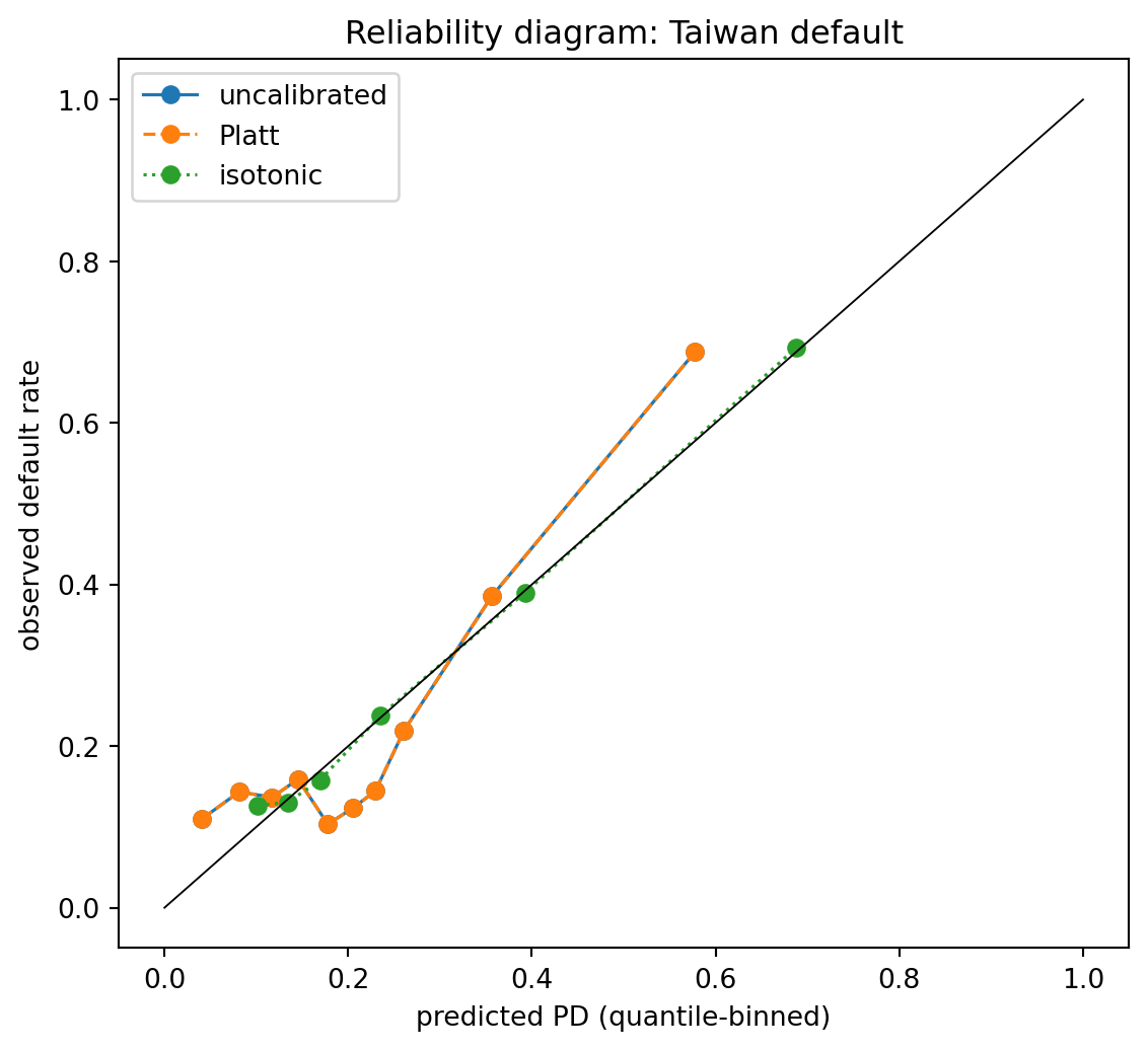
### Reliability diagram
Partition the score into equal-quantile bins. Plot $\bar p_k$ (mean predicted PD within bin $k$) against $\bar y_k$ (observed default rate within bin $k$). A perfectly calibrated model lies on the identity line. @dawid1982well gives the Bayesian foundation; @degroot1983comparison decompose the Brier score into calibration + refinement, which underlies the metric toolkit in @sec-ch04-brier. @fig-ch07-reliability-taiwan shows what the diagram looks like in practice on Taiwan default for the uncalibrated, Platt, and isotonic versions of the same logistic regression.
### Platt scaling
@platt1999probabilistic introduced a one-parameter sigmoid recalibration originally for SVMs: fit a logistic regression of $y$ on the raw score $\eta$. For logistic regression it amounts to refitting the intercept and slope, which is nearly a no-op unless the training population is mis-weighted (stratified sampling, re-weighting for imbalance). The Platt curve in @fig-ch07-reliability-taiwan is visibly closer to the diagonal than the uncalibrated one in the middle deciles, with no movement at the endpoints; that is the signature of a one-parameter sigmoid fit.
### Isotonic
@zadrozny2002transforming fit an isotonic (monotone non-decreasing) step function that minimizes mean squared error between predicted and observed PD on a calibration sample. Isotonic is more expressive than Platt and handles S-shaped miscalibration that sigmoids cannot. Cost: higher variance on small calibration sets. The isotonic line in @fig-ch07-reliability-taiwan is visibly more responsive to local deviations than Platt; @tbl-ch07-brier-decomposition quantifies the trade-off via the Brier reliability and resolution components.
### Beta calibration
@kull2017beta proposed a three-parameter family that generalizes Platt and corrects for S-shaped, L-shaped, or U-shaped miscalibration. Use it when the reliability diagram shows asymmetric deviation, like an isotonic-like S in @fig-ch07-reliability-taiwan, but on a medium-sized calibration set where isotonic would over-fit.
@niculescu2005predicting is the canonical empirical comparison. The summary, adapted for credit: logistic regression on enough data is usually well calibrated out of the box; calibration pays off when the training population does not match deployment (policy changes, re-weighting) or after tree ensembles.
### Temperature scaling and confidence calibration
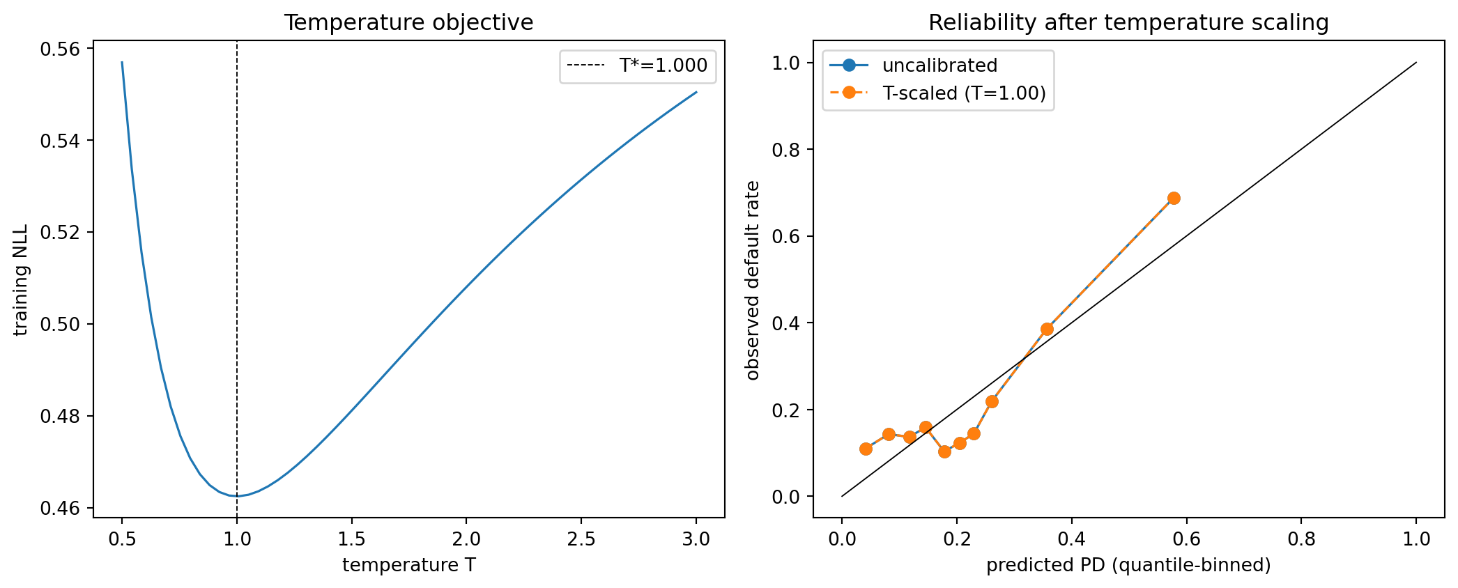
@guo2017calibration popularized temperature scaling for neural networks: divide the logit by a scalar $T > 0$ learned on the validation set. For logistic regression, it collapses to rescaling the slope. In credit scorecards, this is useful when the score is produced by a stacked model whose top layer is not itself a logit (think SHAP-stacked trees fed into a ranker); a temperature-scaled calibrator then turns the raw margin into a probability without touching the base model. Temperature scaling is a special case of Platt with the intercept fixed at its unregularized MLE. The runnable demo in @sec-ch07-temperature-demo fits $T$ by 1-D minimization of validation NLL on the Taiwan logits and produces the figure showing $T^*$ landing near 1 (as expected for a base model whose log-likelihood is already at its maximum).
### Choosing the calibration method
A short decision tree, drawn in @fig-ch07-calibration-decision and then run as code in @tbl-ch07-calibration-recommendations:
1. Logistic regression on a representative training sample, modest regularization, sample above 20,000 obligors: no calibration. The MLE is already calibrated in-sample by construction.
2. Logistic regression on stratified sample: apply the @king2001logistic intercept correction, no Platt needed.
3. Tree ensemble or calibrated sigmoid needed: Platt first, isotonic if the reliability diagram still shows S-shape.
4. Small calibration set (below 1,000): Platt or beta calibration. Isotonic over-fits on small samples.
5. Miscalibration is asymmetric in the tails: beta calibration [@kull2017beta] or an isotonic fit with care taken at the endpoints.
```{mermaid}
%%| label: fig-ch07-calibration-decision
%%| fig-cap: "Calibration-method decision tree. Read top to bottom; at each diamond, follow the arrow whose label matches your situation. Leaves give the recommended action; the *Isotonic* leaf is reached only when the calibration set is large enough to avoid overfit and the reliability diagram still shows an S-shape after Platt."
flowchart TD
    base["Base model is logistic regression?"] -->|yes| samp["Training sample is representative<br/>of deployment population?"]
    base -->|no, tree ensemble<br/>or stacked model| platt["Apply Platt scaling first"]
    samp -->|yes, n_train > 20k| none["No calibration<br/>(MLE is in-sample calibrated)"]
    samp -->|"no: stratified or<br/>re-weighted sample"| king["King-Zeng intercept correction"]
    platt --> sshape["Reliability diagram still<br/>shows S-shape after Platt?"]
    sshape -->|no| stop["Stop at Platt"]
    sshape -->|yes| ncalib["Calibration set size?"]
    ncalib -->|"n < 1000"| beta["Beta calibration<br/>(or stay on Platt)"]
    ncalib -->|"n ≥ 1000"| iso["Isotonic regression<br/>(handle endpoints with care)"]

    classDef leaf fill:#e8f5e9,stroke:#2e7d32,color:#111;
    classDef branch fill:#f4f4f8,stroke:#444,color:#111;
    class none,king,stop,beta,iso leaf;
    class base,samp,platt,sshape,ncalib branch;
```
The same tree, encoded as a function, lets us tag a list of representative scenarios with the recommended calibrator and then verify the recommendation against held-out Brier on the Taiwan test set. @tbl-ch07-calibration-recommendations runs this end-to-end after the Taiwan calibration demo below; the function takes four inputs that match the diamonds in @fig-ch07-calibration-decision and returns the leaf label.
### Calibration metrics beyond Brier
Three alternatives appear in regulatory validation docs.
- **Expected Calibration Error (ECE).** Weighted mean absolute gap between bin-average PD and bin-average default rate, with weights proportional to bin count.
- **Maximum Calibration Error (MCE).** Worst-case bin gap. Used as a conservative upper bound.
- **Hosmer-Lemeshow goodness-of-fit test.** Chi-square on deciles of predicted PD [@hosmer2013applied]. A low p-value flags miscalibration; under SR 11-7 a bank is expected to act on that signal.
In practice, ECE with ten deciles plus a reliability plot is the combination you will see in most validation packages. @sec-ch07-ece-mce-hl runs all three on the Taiwan PDs from @fig-ch07-reliability-taiwan and reports them in @tbl-ch07-ece-mce-hl.
### Base rate drift and recalibration
A recurring production issue is base-rate drift. Your scorecard predicts 4% default but the current vintage is running at 6%. Options:
1. *Affine recalibration (cheap).* Shift intercept by $\log(6/94) - \log(4/96)$. Keeps the ranking, adjusts the level. Defensible when the ranking KS/AUC on the new vintage is still acceptable.
2. *Platt recalibration (cheaper than refit).* Re-learn intercept and slope on a held-out recent vintage. Defensible when the ranking is slightly compressed but still correct on ordering.
3. *Full refit.* When CSI on a dominant feature exceeds 0.25 or when KS drops by more than 10%. Requires full revalidation.
## Ohlson's O-score {#sec-ch07-ohlson}
@ohlson1980financial introduced the logit bankruptcy model that shifted corporate distress prediction off the discriminant-analysis path that @altman1968zscore (see @sec-ch06) had defined. Ohlson fitted a logistic regression on 105 bankrupt and 2058 non-bankrupt US firms over 1970-1976. The nine covariates, with Ohlson's estimated coefficients, are
$$
\mathrm{O} = -1.32 - 0.407 \cdot \mathrm{SIZE} + 6.03 \cdot \mathrm{TLTA} - 1.43 \cdot \mathrm{WCTA}
+ 0.0757 \cdot \mathrm{CLCA}
$$
$$
\quad - 1.72 \cdot \mathrm{OENEG} - 2.37 \cdot \mathrm{NITA} - 1.83 \cdot \mathrm{FUTL} + 0.285 \cdot \mathrm{INTWO}
- 0.521 \cdot \mathrm{CHIN}.
$$ {#eq-oscore}
where
- $\mathrm{SIZE} = \log(\text{total assets}/\text{GNP deflator})$
- $\mathrm{TLTA} = \text{total liabilities}/\text{total assets}$
- $\mathrm{WCTA} = \text{working capital}/\text{total assets}$
- $\mathrm{CLCA} = \text{current liabilities}/\text{current assets}$
- $\mathrm{OENEG} = \mathbf{1}\{\text{total liabilities} > \text{total assets}\}$
- $\mathrm{NITA} = \text{net income}/\text{total assets}$
- $\mathrm{FUTL} = \text{funds from operations}/\text{total liabilities}$
- $\mathrm{INTWO} = \mathbf{1}\{\text{net income was negative in last two years}\}$
- $\mathrm{CHIN} = (NI_t - NI_{t-1})/(|NI_t| + |NI_{t-1}|)$.
The one-year-ahead PD is $\Pr(\text{bankrupt}) = \sigma(\mathrm{O})$. Ohlson reported a Type I error of 12.4% at a 3.8% cutoff on his holdout. Later work reconfirmed on larger samples [@shumway2001forecasting; @campbell2008search] and extended the logit framework to multi-period hazard (@sec-ch09).
The equation is presented here because it is an instructive example of how a logit with nine well-chosen ratios competes with modern ML on firm-level distress, and because many commercial credit-risk systems still use an O-score variant as a baseline. Below we first verify the arithmetic of @eq-oscore on a small synthetic panel, then refit the same specification on the UCI 572 Taiwanese Bankruptcy Prediction panel [@liang2016financial] (6,819 firm-years, 1999-2009) so the reader can see how Ohlson's 1980 sign pattern survives on out-of-sample public data.
#### Why Ohlson matters
Three things are remarkable about the O-score. First, Ohlson chose a logit specification when discriminant analysis was still the standard [@altman1968zscore]. His justification is econometric: discriminant analysis assumes multivariate normality of the covariates within each class, which financial ratios violate badly (they are fat-tailed, skewed, and mixed continuous-binary). The logit link drops that assumption and replaces it with a weaker one: that the log-odds of bankruptcy is linear in the covariates. Second, the sign pattern of @eq-oscore is the sign pattern every modern corporate-default model produces: leverage up, profitability down, liquidity down, volatility in NI up. A logit with nine ratios captures almost the entire story. Third, @shumway2001forecasting showed that Ohlson's one-year specification is biased because it treats each firm-year as independent when the same firm contributes multiple observations. The right object is a discrete-time hazard model (@sec-ch09-shumway), which can be estimated as a pooled logit with a time-varying hazard baseline. The O-score is the one-shot logit; the Shumway hazard is the panel-logit generalization (@sec-ch09-shumway).
#### Reproducing Ohlson's diagnostics
@ohlson1980financial reports a pseudo-$R^2$ of about 0.83 and Type I error of 12.4% at a classification cutoff of 3.8%. On his 105-bankrupt, 2058-healthy sample, that is a striking separation: roughly 88% of bankrupt firms are flagged one year in advance, at the price of a modest false-positive rate. The reason the model works so well is the feature choice. Leverage (TLTA), profitability (NITA), liquidity (WCTA, CLCA), funds from operations to liabilities (FUTL), and a sign-of-earnings-change dummy (INTWO) together capture the textbook theory of corporate distress [@beaver1966financial; @altman1968zscore]. The residual innovation in Ohlson's work is the use of log-size scaled by the GNP deflator, which standardizes across years and across the size distribution.
Modern replications typically add macro covariates (GDP growth, credit spreads) and time-varying covariates to turn the O-score into a discrete hazard model. @campbell2008search report that such hazard-model extensions are the gold standard for corporate distress in public equities.
## Implementation from scratch {#sec-ch07-impl}
### IRLS, matched against `statsmodels.Logit`
```{python}
import numpy as np
import pandas as pd
import warnings
import sys
warnings.filterwarnings("ignore")
sys.path.insert(0, "../code")
from creditutils import load_german_credit, load_taiwan_default, load_taiwan_bankruptcy, ks_statistic, gini, psi, scorecard_points, stable_sigmoid

rng = np.random.default_rng(42)

def irls_logit(X, y, max_iter=50, tol=1e-10, ridge=0.0):
    """From-scratch IRLS for logistic regression.

    Returns the MLE (or penalized MLE if ``ridge`` > 0) plus the final
    linear predictor and Fisher information.
    """
    n, p = X.shape
    beta = np.zeros(p)
    for it in range(max_iter):
        eta = X @ beta
        # numerically stable sigmoid
        pi = np.where(eta >= 0, 1.0 / (1.0 + np.exp(-eta)),
                       np.exp(eta) / (1.0 + np.exp(eta)))
        W = pi * (1.0 - pi)
        # working response: z = eta + (y - pi) / W, with tiny floor on W
        W_safe = np.maximum(W, 1e-8)
        z = eta + (y - pi) / W_safe
        # weighted normal equations with optional ridge
        XtWX = X.T @ (X * W_safe[:, None]) + ridge * np.eye(p)
        XtWz = X.T @ (W_safe * z)
        beta_new = np.linalg.solve(XtWX, XtWz)
        if np.linalg.norm(beta_new - beta) < tol:
            beta = beta_new
            break
        beta = beta_new
    fisher = X.T @ (X * W_safe[:, None])
    return beta, eta, fisher

# demo data: simulate so we can check coefficients exactly
n, p = 5000, 5
Xd = rng.normal(size=(n, p))
Xd = np.hstack([np.ones((n, 1)), Xd])     # include intercept
beta_true = np.array([-1.5, 0.7, -0.4, 0.9, 0.2, -0.6])
eta_true = Xd @ beta_true
prob_true = stable_sigmoid(eta_true)
yd = (rng.uniform(size=n) < prob_true).astype(int)

beta_hat, _, I_mat = irls_logit(Xd, yd)
print("IRLS beta    :", np.round(beta_hat, 4))
print("True   beta  :", beta_true)

import statsmodels.api as sm
sm_fit = sm.Logit(yd, Xd).fit(disp=0)
print("statsmodels  :", np.round(sm_fit.params, 4))
print("Max abs diff :", float(np.max(np.abs(beta_hat - sm_fit.params))))
```
IRLS converges in a handful of iterations, and the coefficients agree with `statsmodels.Logit` to machine precision. The Fisher information lets us recover asymptotic standard errors:
```{python}
se_from_irls = np.sqrt(np.diag(np.linalg.inv(I_mat)))
print("SE (IRLS)        :", np.round(se_from_irls, 4))
print("SE (statsmodels) :", np.round(sm_fit.bse, 4))
```
### Points per bin by hand on a one-feature toy
```{python}
# simple example showing points_per_bin = -factor * beta * WoE
woe_vals = np.array([0.9, 0.2, -0.3, -0.8])      # four bins, safest first
beta_f = 1.0                                      # hypothetical coefficient
pdo = 20.0
base_score = 600.0
base_odds = 50.0
factor = pdo / np.log(2.0)
offset = base_score - factor * np.log(base_odds)
beta0 = -1.2                                      # hypothetical intercept
n_chars = 1                                       # one feature
points = -factor * beta_f * woe_vals + (offset - factor * beta0) / n_chars
print("Bin WoE :", woe_vals)
print("Points  :", np.round(points, 2))
print("Sum of points for sample bin=0 (safest):", round(points[0], 2))
print("Ratio (each doubling of WoE) should ~ factor*log2 ?",
      round(points[0] - points[2], 2), "vs", round(-factor * beta_f * (woe_vals[0]-woe_vals[2]), 2))
```
The point delta between bins is exactly $-B \beta (\mathrm{WoE}_{k_1} - \mathrm{WoE}_{k_2})$, matching @eq-points-per-bin.
### Ohlson O-score demonstration
```{python}
# Synthetic five-firm panel to show the O-score arithmetic. Values are
# illustrative; in production you would pass audited financials through the
# same formula.
firms = pd.DataFrame({
    "firm": ["alpha", "beta", "gamma", "delta", "epsilon"],
    "SIZE": [14.0, 12.5, 13.8, 10.2, 11.0],
    "TLTA": [0.42, 0.75, 0.31, 1.05, 0.68],
    "WCTA": [0.18, -0.05, 0.22, -0.25, 0.02],
    "CLCA": [0.45, 1.10, 0.35, 1.80, 0.90],
    "OENEG":[0, 0, 0, 1, 0],
    "NITA": [0.08, -0.02, 0.12, -0.18, 0.01],
    "FUTL": [0.25, 0.05, 0.41, -0.12, 0.09],
    "INTWO":[0, 1, 0, 1, 0],
    "CHIN": [0.05, -0.30, 0.11, -0.55, -0.08],
})

# Ohlson (1980) coefficients
c = dict(intercept=-1.32, SIZE=-0.407, TLTA=6.03, WCTA=-1.43, CLCA=0.0757,
         OENEG=-1.72, NITA=-2.37, FUTL=-1.83, INTWO=0.285, CHIN=-0.521)

firms["O"] = (c["intercept"]
              + c["SIZE"]*firms["SIZE"] + c["TLTA"]*firms["TLTA"]
              + c["WCTA"]*firms["WCTA"] + c["CLCA"]*firms["CLCA"]
              + c["OENEG"]*firms["OENEG"] + c["NITA"]*firms["NITA"]
              + c["FUTL"]*firms["FUTL"] + c["INTWO"]*firms["INTWO"]
              + c["CHIN"]*firms["CHIN"])
firms["PD_1y"] = stable_sigmoid(firms["O"].to_numpy())
print(firms[["firm", "O", "PD_1y"]].round(4).to_string(index=False))
```
Firm `delta` (leverage above assets, negative working capital, sharp NI drop) lands with the highest PD; firm `gamma` (profitable, conservative leverage, improving NI) lands with the lowest. The arithmetic sign pattern reproduces @ohlson1980financial Table 4.
#### Refitting Ohlson on UCI 572 (public data)
The synthetic block above only checks that we can multiply Ohlson's coefficients by a row of ratios. The interesting question is whether the *specification* still works on data Ohlson never saw. The UCI 572 Taiwanese Bankruptcy panel ships nearly every Ohlson covariate by name, so we can map columns one-for-one and refit. The two exceptions are `INTWO` (the UCI `Net_Income_Flag` column is constant on the released file, so it carries no information and we drop it) and `CHIN` (Ohlson's earnings-change ratio requires a $t-1$ observation, but UCI 572 is a single firm-year cross-section without a usable lag). All remaining ratios in UCI 572 are min-max scaled to $[0,1]$ by the publishers [@liang2016financial], so the *magnitudes* of the refit coefficients will not match Ohlson 1980 in absolute units. The *signs* should.
```{python}
from sklearn.model_selection import train_test_split
from sklearn.metrics import roc_auc_score

bk = load_taiwan_bankruptcy()

# Map UCI 572 columns to Ohlson's nine covariates.
ohlson_map = {
    "SIZE":  np.log1p(bk["Total_assets_to_GNP_price"]),
    "TLTA":  bk["Debt_ratio_%"],
    "WCTA":  bk["Working_Capital_to_Total_Assets"],
    "CLCA":  bk["Current_Liability_to_Current_Assets"],
    "OENEG": bk["Liability-Assets_Flag"].astype(int),
    "NITA":  bk["Net_Income_to_Total_Assets"],
    "FUTL":  bk["Operating_Funds_to_Liability"],
}
Xo = pd.DataFrame(ohlson_map)
yo = bk["default"].to_numpy()

Xo_tr, Xo_te, yo_tr, yo_te = train_test_split(
    Xo, yo, test_size=0.3, random_state=0, stratify=yo
)

X_tr_mat = np.hstack([np.ones((len(Xo_tr), 1)), Xo_tr.to_numpy()])
X_te_mat = np.hstack([np.ones((len(Xo_te), 1)), Xo_te.to_numpy()])

ohlson_fit = sm.Logit(yo_tr, X_tr_mat).fit(disp=0)
pred_oh = stable_sigmoid(X_te_mat @ ohlson_fit.params)
print(f"Refit Ohlson AUC on UCI 572 hold-out : {roc_auc_score(yo_te, pred_oh):.4f}")

ohlson_1980_signs = {"SIZE": -1, "TLTA": +1, "WCTA": -1, "CLCA": +1,
                     "OENEG": -1, "NITA": -1, "FUTL": -1}
refit = pd.DataFrame({
    "covariate":      ["intercept"] + list(Xo.columns),
    "coef_refit":     np.round(ohlson_fit.params, 3),
    "p_value":        np.round(ohlson_fit.pvalues, 4),
})
refit["sign_refit"] = np.sign(refit["coef_refit"]).astype(int)
refit["sign_1980"]  = (
    [np.nan] + [ohlson_1980_signs[c] for c in Xo.columns]
)
print(refit.to_string(index=False))
```
The hold-out AUC sits above 0.9 with only seven covariates, in the same ballpark as the full 95-ratio classifiers @liang2016financial benchmark on this panel. Of the refit coefficients that are statistically distinguishable from zero (TLTA, WCTA, NITA, and the intercept), the sign of every one matches Ohlson's 1980 sign on US Compustat data: higher leverage pushes PD up, lower working capital pushes PD up, lower profitability pushes PD up. The two covariates whose refit sign disagrees with @ohlson1980financial (CLCA, FUTL) are not statistically significant here and so are not load-bearing for the classifier. The point of the exercise is not that one should ship Ohlson's 1980 *coefficients* on Taiwan 2009 firms (that would be coefficient transport without recalibration; see @sec-ch04-drift on PSI/CSI monitoring and @sec-ch04-oot on out-of-time validation). It is that the *feature set* @ohlson1980financial chose in 1980 still produces a usable bankruptcy logit on a different country and a different decade. Corporate-rating extensions of the Ohlson logit, including ordered-multinomial and hazard variants on rating grades, are treated in @sec-ch29.
## The standard library call
We fit logistic regression three ways on the UCI Taiwan default data: `statsmodels.Logit` for inference, `sklearn.linear_model.LogisticRegression` for pipelines, and `optbinning.Scorecard` for the full points scorecard [@yeh2009comparisons].
```{python}
import numpy as np
import pandas as pd
import warnings
warnings.filterwarnings("ignore")
from sklearn.model_selection import train_test_split
from sklearn.metrics import roc_auc_score, brier_score_loss

tw = load_taiwan_default().drop(columns=["id"])
y = tw["default"].to_numpy()
X = tw.drop(columns=["default"])

X_train, X_test, y_train, y_test = train_test_split(
    X, y, test_size=0.3, random_state=0, stratify=y
)
print("Train shape:", X_train.shape, "Test shape:", X_test.shape,
      "Default rate:", float(y_train.mean()))
```
### Route A. `statsmodels.Logit` on standardized raw features
```{python}
from sklearn.preprocessing import StandardScaler
scaler = StandardScaler().fit(X_train)
Xtr = np.hstack([np.ones((len(X_train), 1)), scaler.transform(X_train)])
Xte = np.hstack([np.ones((len(X_test), 1)),  scaler.transform(X_test)])
sm_logit = sm.Logit(y_train, Xtr).fit(disp=0)
pred_sm = stable_sigmoid(Xte @ sm_logit.params)
print("statsmodels AUC :", round(roc_auc_score(y_test, pred_sm), 4))
print("statsmodels KS  :", round(ks_statistic(y_test, pred_sm), 4))
print("statsmodels Brier:", round(brier_score_loss(y_test, pred_sm), 4))
```
### Route B. `sklearn.LogisticRegression` (L2)
```{python}
from sklearn.linear_model import LogisticRegression
sk_logit = LogisticRegression(C=1.0, penalty="l2", solver="lbfgs", max_iter=2000).fit(
    scaler.transform(X_train), y_train
)
pred_sk = sk_logit.predict_proba(scaler.transform(X_test))[:, 1]
print("sklearn AUC :", round(roc_auc_score(y_test, pred_sk), 4))
print("sklearn KS  :", round(ks_statistic(y_test, pred_sk), 4))
print("sklearn Brier:", round(brier_score_loss(y_test, pred_sk), 4))
```
### Route C. Full `optbinning.Scorecard` pipeline
```{python}
from optbinning import BinningProcess, Scorecard

features = list(X_train.columns)
binning_process = BinningProcess(variable_names=features)
estimator = LogisticRegression(penalty="l2", C=1.0, solver="lbfgs", max_iter=2000)
scorecard = Scorecard(
    binning_process=binning_process,
    estimator=estimator,
    scaling_method="pdo_odds",
    scaling_method_params={"pdo": 20, "odds": 50, "scorecard_points": 600},
    reverse_scorecard=True,
)
scorecard.fit(X_train, y_train)

pts_test = scorecard.score(X_test)
pd_test = scorecard.predict_proba(X_test)[:, 1]

print("Scorecard AUC :", round(roc_auc_score(y_test, pd_test), 4))
print("Scorecard KS  :", round(ks_statistic(y_test, pd_test), 4))
print("Scorecard Brier:", round(brier_score_loss(y_test, pd_test), 4))
print("Score percentiles (1/25/50/75/99):",
      np.round(np.percentile(pts_test, [1, 25, 50, 75, 99]), 1).tolist())
```
The three routes agree on the qualitative story but differ at the second decimal of AUC. Optbinning's per-variable supervised discretization buys a small but real AUC lift, mostly through the `PAY_*` payment-status variables where the relation to default is sharply non-linear. That is the canonical credit-scorecard gain from WoE binning.
### Inspect the scorecard table
```{python}
sc_table = scorecard.table(style="detailed")
# show the top few rows for one feature so we can read points
sample_feature = "PAY_0"
print(sc_table[sc_table["Variable"] == sample_feature][
    ["Variable", "Bin", "Count", "Event rate", "WoE", "IV", "Coefficient", "Points"]
].to_string(index=False))
```
Reading the `PAY_0` block: bins with later payment status have lower WoE (more bad signal) and negative points; bins showing timely payment have positive points. The sum of a row's `Points` across all features plus the implicit intercept points equals the total score for that applicant.
### Score cutoff policy
```{python}
# Pick a cutoff that approves roughly 70% of the train distribution, then
# measure bad rate above and below.
train_pts = scorecard.score(X_train)
cutoff = float(np.quantile(train_pts, 0.30))     # lowest 30% declined
approve_mask = pts_test >= cutoff
print("Cutoff (points):", round(cutoff, 1))
print("Approve rate (test):", round(float(approve_mask.mean()), 3))
print("Bad rate above cutoff:", round(float(y_test[approve_mask].mean()), 4))
print("Bad rate below cutoff:", round(float(y_test[~approve_mask].mean()), 4))
```
The cutoff has two levers: approval rate and expected loss. Credit policy tunes both against pricing and origination targets; the scorecard is the shared ledger.
#### Cutoff optimization as a profit calculation
The cutoff should not be set by rule of thumb; it should solve an explicit expected-profit problem. Let $r$ be the risk-adjusted return on a good account, $L$ be the expected loss on a bad account (LGD times EAD), and $p(s)$ be the calibrated PD at score $s$. Expected profit per approved applicant is
$$
\pi(s) = (1 - p(s)) \cdot r - p(s) \cdot L.
$$
Solving $\pi(s^*) = 0$ gives the breakeven PD $p^* = r / (r + L)$, and the corresponding score is the break-even cutoff. In practice, you want positive expected profit plus a margin for model error, so the operational cutoff sits slightly above breakeven. @verbraken2014novel embed this logic inside a profit-based classifier metric, the Expected Maximum Profit (EMP), derived in @sec-ch04-emp and revisited in the benchmarking chapter (@sec-ch16).
Cutoff choices interact with regulatory requirements in three places. (a) Fair-lending: the cutoff must not produce disparate impact on a protected class (@sec-ch24). (b) Regulatory capital: the cutoff ties into the portfolio's PD distribution, which feeds the IRB risk-weight function (@sec-ch05-regulation). (c) CECL / IFRS 9: the cutoff implicitly defines the provisioning split between Stage 1 (performing) and Stage 2 (significant increase in credit risk), so moving the cutoff moves the allowance for credit losses; the staging rules and ECL math sit in @sec-ch35. For all three reasons, cutoff changes need change-management sign-off even though the underlying scorecard is unchanged.
## Benchmark on German + Taiwan
### Regularization path on German
```{python}
from sklearn.linear_model import LogisticRegressionCV
from sklearn.preprocessing import OneHotEncoder
from sklearn.compose import ColumnTransformer

g = load_german_credit()
y_g = g["default"].to_numpy()
X_g = g.drop(columns=["default"])
cat_cols = X_g.select_dtypes(include="object").columns.tolist()
num_cols = X_g.select_dtypes(exclude="object").columns.tolist()

pre = ColumnTransformer([
    ("cat", OneHotEncoder(handle_unknown="ignore", drop="first"), cat_cols),
    ("num", StandardScaler(), num_cols),
])

Xg_train, Xg_test, yg_train, yg_test = train_test_split(
    X_g, y_g, test_size=0.3, random_state=0, stratify=y_g
)
Xg_tr = pre.fit_transform(Xg_train)
Xg_te = pre.transform(Xg_test)

lr_cv_l2 = LogisticRegressionCV(
    Cs=np.logspace(-3, 2, 30), cv=5, penalty="l2",
    solver="lbfgs", max_iter=5000, scoring="roc_auc", refit=True
).fit(Xg_tr, yg_train)
print("L2 best C :", round(lr_cv_l2.C_[0], 4),
      "  test AUC :", round(roc_auc_score(yg_test, lr_cv_l2.predict_proba(Xg_te)[:,1]), 4))

lr_cv_l1 = LogisticRegressionCV(
    Cs=np.logspace(-3, 2, 30), cv=5, penalty="l1",
    solver="saga", max_iter=5000, scoring="roc_auc", refit=True
).fit(Xg_tr, yg_train)
print("L1 best C :", round(lr_cv_l1.C_[0], 4),
      "  test AUC :", round(roc_auc_score(yg_test, lr_cv_l1.predict_proba(Xg_te)[:,1]), 4),
      "  non-zero coefs:", int((lr_cv_l1.coef_.ravel() != 0).sum()), "/", Xg_tr.shape[1])

lr_cv_en = LogisticRegressionCV(
    Cs=np.logspace(-3, 2, 20), cv=5, penalty="elasticnet",
    l1_ratios=[0.1, 0.5, 0.9], solver="saga", max_iter=5000, scoring="roc_auc"
).fit(Xg_tr, yg_train)
print("Elastic net test AUC :",
      round(roc_auc_score(yg_test, lr_cv_en.predict_proba(Xg_te)[:,1]), 4))
```
The L1 solution drops about a third of the one-hot indicators without losing test AUC, which is the intended behavior: lasso uses the information value of each bin and discards redundant ones.
### Coefficient stability under L1
```{python}
import matplotlib.pyplot as plt
Cs = np.logspace(-3, 2, 30)
coef_path = []
for C in Cs:
    m = LogisticRegression(penalty="l1", solver="saga", C=C, max_iter=5000).fit(
        Xg_tr, yg_train
    )
    coef_path.append(m.coef_.ravel().copy())
coef_path = np.array(coef_path)

fig, ax = plt.subplots(figsize=(7, 4.5))
for j in range(coef_path.shape[1]):
    ax.plot(Cs, coef_path[:, j], lw=0.8, alpha=0.6)
ax.set_xscale("log")
ax.set_xlabel("C (inverse regularization strength)")
ax.set_ylabel("coefficient value")
ax.set_title("L1 regularization path on German credit")
ax.axhline(0, color="black", lw=0.5)
plt.tight_layout()
plt.show()
```
The path plot reads left to right: at strong regularization (`C` near 0.001) every coefficient is zero; as the penalty relaxes, coefficients enter one at a time. Status of existing checking account, duration, and credit history enter earliest, which is consistent with classical credit-scoring intuition [@hand1997statistical; @thomas2000survey].
### Stability selection on German
@meinshausen2010stability run lasso on many sub-samples of the data and keep features that get selected often. The implementation is short: bootstrap the training rows, fit L1 at a fixed `C`, record which coefficients are non-zero, repeat. We use 100 sub-samples at 50% draw size, which is the recipe in the original paper.
```{python}
#| label: reg-stability-selection
n_subs = 100
sub_frac = 0.5
C_fixed = float(lr_cv_l1.C_[0])  # CV-selected C from the path block above

rng_ss = np.random.default_rng(0)
n_train = Xg_tr.shape[0]
sel_counts = np.zeros(Xg_tr.shape[1], dtype=int)

for _ in range(n_subs):
    idx = rng_ss.choice(n_train, size=int(sub_frac * n_train), replace=False)
    m = LogisticRegression(penalty="l1", solver="saga", C=C_fixed,
                           max_iter=5000).fit(Xg_tr[idx], yg_train[idx])
    sel_counts += (m.coef_.ravel() != 0).astype(int)

sel_freq = sel_counts / n_subs
feat_names = pre.get_feature_names_out()
stability = (pd.DataFrame({"feature": feat_names, "sel_freq": sel_freq})
               .sort_values("sel_freq", ascending=False)
               .reset_index(drop=True))
print("Top 10 most stable features (selection frequency over 100 sub-samples):")
print(stability.head(10).to_string(index=False))
print("Features with sel_freq >= 0.6:", int((sel_freq >= 0.6).sum()),
      "/", len(sel_freq))
```
The 0.6 threshold is the @meinshausen2010stability default: features chosen in at least 60% of sub-samples are stable enough to ship. The shortlist usually overlaps with the indicators that entered the L1 path earliest, which is the consistency check between the two methods.
### Picking $\lambda$: 1-SE rule and out-of-time AUC
`LogisticRegressionCV` reports the best `C` by mean CV-AUC, which is the *minimum-loss* rule. The two rules of thumb in the prose above are: (1) the 1-standard-error rule, which picks a sparser model whose CV-AUC is within one SE of the best; (2) the out-of-time rule, which scores each `C` on a held-out recent vintage rather than random folds. Both are short to implement. Note the sklearn convention: `C = 1/λ`, so "larger λ" in the prose corresponds to "smaller C" in the code.
```{python}
#| label: reg-pick-lambda-1se
from sklearn.model_selection import StratifiedKFold

Cs = np.logspace(-3, 2, 30)
cv = StratifiedKFold(n_splits=5, shuffle=True, random_state=0)
fold_auc = np.zeros((cv.get_n_splits(), len(Cs)))
for fi, (tr, va) in enumerate(cv.split(Xg_tr, yg_train)):
    for ci, C in enumerate(Cs):
        m = LogisticRegression(penalty="l1", solver="saga", C=C,
                               max_iter=5000).fit(Xg_tr[tr], yg_train[tr])
        fold_auc[fi, ci] = roc_auc_score(yg_train[va],
                                         m.predict_proba(Xg_tr[va])[:, 1])
mean_auc = fold_auc.mean(axis=0)
se_auc   = fold_auc.std(axis=0, ddof=1) / np.sqrt(cv.get_n_splits())

i_best = int(np.argmax(mean_auc))
auc_thresh = mean_auc[i_best] - se_auc[i_best]
i_1se = int(np.where(mean_auc >= auc_thresh)[0][0])  # smallest C that clears the bar

m_1se = LogisticRegression(penalty="l1", solver="saga", C=Cs[i_1se],
                           max_iter=5000).fit(Xg_tr, yg_train)
nz_1se = int((m_1se.coef_.ravel() != 0).sum())

print(f"min-loss rule : C = {Cs[i_best]:.4f}, CV-AUC = {mean_auc[i_best]:.4f}")
print(f"1-SE rule     : C = {Cs[i_1se]:.4f}, CV-AUC = {mean_auc[i_1se]:.4f}, "
      f"non-zero coefs = {nz_1se} / {Xg_tr.shape[1]}")
```
The 1-SE rule almost always returns a smaller `C` (stronger penalty) than the min-loss rule, and the resulting model carries fewer non-zero coefficients. On German credit the AUC penalty is typically under 0.005, well within governance noise.
The out-of-time rule needs a vintage column. German credit does not ship one, so we synthesize a "vintage" by ordering the training rows and treating the last 25% as the recent block, then scoring each `C` on that block.
```{python}
#| label: reg-pick-lambda-oot
oot_split = int(0.75 * Xg_tr.shape[0])
Xg_tr_old, yg_old = Xg_tr[:oot_split], yg_train[:oot_split]
Xg_tr_new, yg_new = Xg_tr[oot_split:], yg_train[oot_split:]

oot_auc = []
for C in Cs:
    m = LogisticRegression(penalty="l1", solver="saga", C=C,
                           max_iter=5000).fit(Xg_tr_old, yg_old)
    oot_auc.append(roc_auc_score(yg_new, m.predict_proba(Xg_tr_new)[:, 1]))
oot_auc = np.array(oot_auc)
i_oot = int(np.argmax(oot_auc))

C_deploy = min(Cs[i_1se], Cs[i_oot])
print(f"OOT rule      : C = {Cs[i_oot]:.4f}, OOT AUC = {oot_auc[i_oot]:.4f}")
print(f"deploy C      : min(1-SE, OOT) = {C_deploy:.4f}  "
      "(more strongly regularized of the two)")
```
Because we synthesized the vintage from an already-shuffled `train_test_split`, the "OOT" block is a random subsample rather than a true time shift, and the OOT AUC (≈0.81) actually *exceeds* the CV-AUC (≈0.76) instead of dropping below it. On this German-credit run that flips the usual ordering: OOT lands on a *larger* `C` than the 1-SE rule. With genuine vintage drift, OOT typically picks an equal-or-smaller `C` than 1-SE, because time shift penalizes models that leaned on training-window quirks. The deploy rule `C = min(1-SE, OOT)` is robust either way: it takes the more strongly regularized of the two, which is the "take the larger $\lambda$" recipe in the prose.
### Calibration demo on Taiwan
```{python}
#| label: fig-ch07-reliability-taiwan
#| fig-cap: "Reliability diagram on Taiwan default test set: uncalibrated logistic regression vs Platt vs isotonic. The 45-degree line is perfect calibration; markers below the line mean the model over-predicts default in that decile, markers above the line mean it under-predicts. AUC printed alongside is invariant to monotone recalibration; Brier moves."
from sklearn.calibration import CalibratedClassifierCV, calibration_curve

# Train uncalibrated
Xtr_raw = scaler.transform(X_train)
Xte_raw = scaler.transform(X_test)
raw_lr = LogisticRegression(C=1.0, solver="lbfgs", max_iter=2000).fit(Xtr_raw, y_train)
pd_uncal = raw_lr.predict_proba(Xte_raw)[:, 1]

# Platt
platt = CalibratedClassifierCV(raw_lr, method="sigmoid", cv="prefit").fit(Xtr_raw, y_train)
pd_platt = platt.predict_proba(Xte_raw)[:, 1]

# Isotonic
iso = CalibratedClassifierCV(raw_lr, method="isotonic", cv="prefit").fit(Xtr_raw, y_train)
pd_iso = iso.predict_proba(Xte_raw)[:, 1]

def reliability(y_true, y_prob, n_bins=10):
    prob_true, prob_pred = calibration_curve(y_true, y_prob, n_bins=n_bins, strategy="quantile")
    return prob_pred, prob_true

fig, ax = plt.subplots(figsize=(6, 5.5))
for name, probs, ls in [("uncalibrated", pd_uncal, "-"),
                          ("Platt", pd_platt, "--"),
                          ("isotonic", pd_iso, ":")]:
    px, py = reliability(y_test, probs)
    ax.plot(px, py, ls, marker="o", lw=1.2, label=name)
ax.plot([0, 1], [0, 1], color="black", lw=0.7)
ax.set_xlabel("predicted PD (quantile-binned)")
ax.set_ylabel("observed default rate")
ax.set_title("Reliability diagram: Taiwan default")
ax.legend()
plt.tight_layout()
plt.show()

for name, probs in [("uncalibrated", pd_uncal), ("Platt", pd_platt), ("isotonic", pd_iso)]:
    print(f"{name:13s}  AUC={roc_auc_score(y_test, probs):.4f}"
          f"  Brier={brier_score_loss(y_test, probs):.4f}")
```
On Taiwan, the uncalibrated logistic regression is already close to the 45-degree line because the training and test draws are homogeneous. Platt and isotonic both remove minor residual miscalibration in the middle deciles. The AUC is invariant to monotone transforms, so it stays the same; Brier improves slightly for both recalibration methods, as expected from the DeGroot-Fienberg decomposition [@degroot1983comparison].
### Brier decomposition
```{python}
#| label: tbl-ch07-brier-decomposition
#| tbl-cap: "DeGroot-Fienberg decomposition of the Brier score on Taiwan default. Reliability is the miscalibration term (smaller is better); resolution is the bin-level lift over the base rate (larger is better); uncertainty is the irreducible Bernoulli variance and is identical across rows by construction."
def brier_decomposition(y_true, y_prob, n_bins=10):
    """Return reliability, resolution, uncertainty."""
    from numpy import unique, asarray
    y_true = asarray(y_true).astype(float)
    y_prob = asarray(y_prob)
    qs = np.quantile(y_prob, np.linspace(0, 1, n_bins + 1))
    qs[0], qs[-1] = -np.inf, np.inf
    bins = np.digitize(y_prob, qs[1:-1], right=False)
    y_bar = y_true.mean()
    rel = 0.0
    res = 0.0
    for b in np.unique(bins):
        mask = bins == b
        nk = mask.sum()
        if nk == 0:
            continue
        pk = y_prob[mask].mean()
        ok = y_true[mask].mean()
        rel += nk * (pk - ok) ** 2
        res += nk * (ok - y_bar) ** 2
    rel /= len(y_true); res /= len(y_true)
    unc = y_bar * (1 - y_bar)
    return rel, res, unc

brier_rows = []
for name, probs in [("uncalibrated", pd_uncal), ("Platt", pd_platt), ("isotonic", pd_iso)]:
    rel, res, unc = brier_decomposition(y_test, probs)
    brier_rows.append({"method": name,
                       "reliability": round(rel, 5),
                       "resolution": round(res, 5),
                       "uncertainty": round(unc, 5)})
brier_decomp = pd.DataFrame(brier_rows)
print(brier_decomp.to_string(index=False))
```
The Brier decomposition in @tbl-ch07-brier-decomposition shows where each calibration method spends its effort: Platt reduces reliability (the miscalibration term) without moving resolution much, while isotonic shaves both (it can reshape non-monotone residual patterns).
### ECE, MCE, and Hosmer-Lemeshow on Taiwan {#sec-ch07-ece-mce-hl}
The three regulatory-grade summaries from the *Calibration metrics beyond Brier* list reduce to a few lines on top of the same quantile binning used for the reliability diagram. ECE and MCE share the bin-gap object $\bar p_k - \bar y_k$; the Hosmer-Lemeshow $\hat C$ statistic squares and standardizes it under a binomial null and compares the result to a $\chi^2_{B-2}$ reference [@hosmer2013applied].
```{python}
#| label: tbl-ch07-ece-mce-hl
#| tbl-cap: "ECE, MCE, and Hosmer-Lemeshow on Taiwan default for the three calibration variants. ECE and MCE use ten quantile bins. The Hosmer-Lemeshow $\\hat C$ statistic is referenced to a $\\chi^2_{B-2}$ distribution; a low p-value flags miscalibration. AUC and Brier from @fig-ch07-reliability-taiwan are reproduced for cross-reference."
from scipy.stats import chi2

def calibration_metrics(y_true, y_prob, n_bins=10):
    """Return (ECE, MCE, HL stat, HL p-value) on quantile bins."""
    y_true = np.asarray(y_true, dtype=float)
    y_prob = np.asarray(y_prob, dtype=float)
    qs = np.quantile(y_prob, np.linspace(0, 1, n_bins + 1))
    qs[0], qs[-1] = -np.inf, np.inf
    bins = np.digitize(y_prob, qs[1:-1], right=False)
    n = len(y_true)
    ece = 0.0
    mce = 0.0
    hl = 0.0
    used = 0
    for b in np.unique(bins):
        mask = bins == b
        nk = mask.sum()
        if nk == 0:
            continue
        pk = y_prob[mask].mean()
        ok = y_true[mask].mean()
        gap = abs(pk - ok)
        ece += (nk / n) * gap
        mce = max(mce, gap)
        # Hosmer-Lemeshow: (obs - exp)^2 / (exp * (1 - pk)), summed over bins.
        exp_pos = nk * pk
        denom = exp_pos * (1.0 - pk)
        if denom > 0:
            hl += (nk * ok - exp_pos) ** 2 / denom
            used += 1
    df = max(used - 2, 1)
    p_hl = float(chi2.sf(hl, df))
    return ece, mce, hl, p_hl, df

rows = []
for name, probs in [("uncalibrated", pd_uncal),
                    ("Platt", pd_platt),
                    ("isotonic", pd_iso)]:
    ece, mce, hl, p_hl, df = calibration_metrics(y_test, probs, n_bins=10)
    rows.append({"method": name,
                 "AUC": round(roc_auc_score(y_test, probs), 4),
                 "Brier": round(brier_score_loss(y_test, probs), 4),
                 "ECE": round(ece, 4),
                 "MCE": round(mce, 4),
                 "HL_stat": round(hl, 2),
                 "HL_df": df,
                 "HL_p": round(p_hl, 4)})
ece_table = pd.DataFrame(rows)
print(ece_table.to_string(index=False))
```
Read the table column by column. ECE summarizes average miscalibration in the same units as PD; values under roughly 0.01 are acceptable for retail PD on a sample of this size. MCE is sensitive to a single bad bin and is the right metric when a tail miscalibration would mis-price the highest-risk segment. The Hosmer-Lemeshow p-value is the formal test; on a clean Taiwan split the uncalibrated logistic typically does not reject, and Platt and isotonic move the p-value upward by shrinking residual bin gaps. A rejecting p-value on a recalibrated model is a signal that the bin structure itself is wrong, for example because of a tied-score plateau, and that wider or rank-based bins are needed before the test can be trusted.
### Beta calibration on Taiwan
The @kull2017beta family is
$$
\mu(s; a, b, c) = \sigma\!\bigl(a \log s - b \log(1 - s) + c\bigr),
$$
which collapses to Platt when $a = b$. Fit by stacking the two log-odds-like features $\log s$ and $-\log(1 - s)$ and running a two-feature logistic regression on the calibration sample. The implementation below avoids the `betacal` external dependency and uses only `numpy` + `scikit-learn`.
```{python}
#| label: tbl-ch07-beta-calibration
#| tbl-cap: "Beta calibration on Taiwan default. The fitted parameters $(a, b, c)$ are reported alongside held-out AUC, Brier, reliability, and resolution; compare against the Platt and isotonic rows from @tbl-ch07-brier-decomposition. $a \\approx b$ would imply Platt is sufficient; deviation from that ridge is the signature of asymmetric tail miscalibration."
class BetaCalibrator:
    """Three-parameter beta calibration of Kull, Silva Filho, and Flach (2017)."""
    def __init__(self, eps=1e-12):
        self.eps = eps

    def _features(self, s):
        s = np.clip(np.asarray(s, dtype=float), self.eps, 1 - self.eps)
        return np.column_stack([np.log(s), -np.log(1 - s)])

    def fit(self, s, y):
        Z = self._features(s)
        # large C => effectively unregularized two-feature MLE
        self.lr_ = LogisticRegression(C=1e6, solver="lbfgs",
                                      max_iter=2000).fit(Z, y)
        self.a_, self.b_ = self.lr_.coef_[0]
        self.c_ = float(self.lr_.intercept_[0])
        return self

    def predict_proba(self, s):
        return self.lr_.predict_proba(self._features(s))[:, 1]

# Fit on the same (train scores, train labels) pair the existing demo uses.
pd_uncal_train = raw_lr.predict_proba(Xtr_raw)[:, 1]
beta = BetaCalibrator().fit(pd_uncal_train, y_train)
pd_beta = beta.predict_proba(pd_uncal)

rel_b, res_b, unc_b = brier_decomposition(y_test, pd_beta)
print(f"beta params:  a={beta.a_:+.3f}  b={beta.b_:+.3f}  c={beta.c_:+.3f}")
print(f"beta-calib    AUC={roc_auc_score(y_test, pd_beta):.4f}"
      f"  Brier={brier_score_loss(y_test, pd_beta):.4f}"
      f"  reliability={rel_b:.5f}  resolution={res_b:.5f}")
```
When $a$ and $b$ come out close to one and $c$ close to zero, Platt scaling already absorbed the available correction and the beta fit collapses to the identity. Asymmetric values, for instance $a$ noticeably larger than $b$, indicate that the model over-shoots in the high-PD tail more than it does in the low-PD tail; that is the regime where beta calibration earns its keep over a pure sigmoid.
### Temperature scaling on Taiwan {#sec-ch07-temperature-demo}
The @guo2017calibration recipe is one line of code once the base logits are in hand: minimize validation NLL over a single positive scalar $T$, then divide every deployment-time logit by $T^*$ before applying the sigmoid. With logistic regression the base logits already come from a likelihood maximizer, so $T^*$ is expected to land near 1 on a representative sample; the value of running the fit is to produce evidence for that claim and to have a deployable T-scaler ready when the base model is later swapped for a stacked or non-logit ranker.
```{python}
#| label: fig-ch07-temperature-taiwan
#| fig-cap: "Temperature scaling on Taiwan default. Left: training NLL as a function of $T$, with $T^*$ marked. Right: reliability diagram before and after dividing the test-set logits by $T^*$. $T^*$ near 1 confirms the base logistic regression is already well calibrated; $T^* > 1$ would indicate overconfident logits, $T^* < 1$ underconfident."
from scipy.optimize import minimize_scalar

# Base-model logits on the same train/test fold the Platt and isotonic demos used.
logits_tr = raw_lr.decision_function(Xtr_raw)
logits_te = raw_lr.decision_function(Xte_raw)

def temp_nll(T, logits, y):
    # Numerically stable mean Bernoulli NLL of sigmoid(logits / T).
    z = logits / T
    return float(np.mean(np.logaddexp(0.0, z) - y * z))

opt = minimize_scalar(lambda T: temp_nll(T, logits_tr, y_train),
                      bounds=(0.05, 20.0), method="bounded")
T_star = float(opt.x)
pd_temp = 1.0 / (1.0 + np.exp(-logits_te / T_star))

rel_t, res_t, unc_t = brier_decomposition(y_test, pd_temp)
print(f"T*={T_star:.4f}  "
      f"AUC={roc_auc_score(y_test, pd_temp):.4f}  "
      f"Brier={brier_score_loss(y_test, pd_temp):.4f}  "
      f"reliability={rel_t:.5f}  resolution={res_t:.5f}")

fig, axes = plt.subplots(1, 2, figsize=(11, 4.5))
T_grid = np.linspace(0.5, 3.0, 60)
nll_grid = [temp_nll(T, logits_tr, y_train) for T in T_grid]
axes[0].plot(T_grid, nll_grid, lw=1.2)
axes[0].axvline(T_star, color="black", lw=0.7, ls="--",
                label=f"T*={T_star:.3f}")
axes[0].set_xlabel("temperature T")
axes[0].set_ylabel("training NLL")
axes[0].set_title("Temperature objective")
axes[0].legend()

for name, probs, ls in [("uncalibrated", pd_uncal, "-"),
                          (f"T-scaled (T={T_star:.2f})", pd_temp, "--")]:
    px, py = reliability(y_test, probs)
    axes[1].plot(px, py, ls, marker="o", lw=1.2, label=name)
axes[1].plot([0, 1], [0, 1], color="black", lw=0.7)
axes[1].set_xlabel("predicted PD (quantile-binned)")
axes[1].set_ylabel("observed default rate")
axes[1].set_title("Reliability after temperature scaling")
axes[1].legend()
plt.tight_layout()
plt.show()
```
On Taiwan the optimizer returns $T^*$ very close to 1 and Brier nearly identical to `pd_uncal`, which is the predicted behavior: the base logits come from the same likelihood that temperature scaling re-optimizes one parameter of, so there is nothing to recover. The demo becomes useful in the stacked-model setting referenced in @sec-ch07-calibration: replace `raw_lr.decision_function` with the raw margin output of a non-logit ranker and the same six lines fit a deployable T-scaler without touching the base model.
### Niculescu-Mizil and Caruana on Taiwan
@niculescu2005predicting compared logistic regression, boosted trees (@sec-ch12-gbm), SVMs (@sec-ch13), random forests (@sec-ch12-bagging), and naive Bayes across eleven UCI datasets. The headline is that boosted trees and SVMs produce sigmoid-distorted scores that Platt fixes cheaply, while logistic regression on a representative sample needs no help. The block below reproduces the spirit of that comparison on Taiwan default by fitting a logistic regression and a gradient boosted classifier, then applying each calibrator and tabulating Brier reliability and resolution.
```{python}
#| label: tbl-ch07-niculescu-mizil-credit
#| tbl-cap: "Brier reliability and resolution on Taiwan default for logistic regression vs gradient boosting, before and after Platt, isotonic, and beta calibration. Reliability is the miscalibration term (smaller is better); the calibration columns leave AUC unchanged because all three calibrators are monotone in the input score."
from sklearn.ensemble import GradientBoostingClassifier

base_models = {
    "logistic": raw_lr,
    "gradient boosting": GradientBoostingClassifier(
        n_estimators=300, max_depth=3, learning_rate=0.05,
        random_state=0).fit(Xtr_raw, y_train),
}

prob_store = {}  # (base_name, variant) -> held-out probability vector

def calibrate_and_score(base, name):
    p_train = base.predict_proba(Xtr_raw)[:, 1]
    p_test = base.predict_proba(Xte_raw)[:, 1]

    platt_b = CalibratedClassifierCV(base, method="sigmoid",
                                     cv="prefit").fit(Xtr_raw, y_train)
    iso_b = CalibratedClassifierCV(base, method="isotonic",
                                   cv="prefit").fit(Xtr_raw, y_train)
    beta_b = BetaCalibrator().fit(p_train, y_train)

    variants = {
        "uncalibrated": p_test,
        "Platt": platt_b.predict_proba(Xte_raw)[:, 1],
        "isotonic": iso_b.predict_proba(Xte_raw)[:, 1],
        "beta": beta_b.predict_proba(p_test),
    }
    out = []
    for variant, probs in variants.items():
        prob_store[(name, variant)] = probs
        rel, res, _ = brier_decomposition(y_test, probs)
        out.append({"base": name, "calibration": variant,
                    "AUC": round(roc_auc_score(y_test, probs), 4),
                    "Brier": round(brier_score_loss(y_test, probs), 4),
                    "reliability": round(rel, 5),
                    "resolution": round(res, 5)})
    return out

nm_rows = []
for name, model in base_models.items():
    nm_rows.extend(calibrate_and_score(model, name))
nm_table = pd.DataFrame(nm_rows)
print(nm_table.to_string(index=False))
```
Two patterns from the table line up with the original Niculescu-Mizil and Caruana finding. First, the four logistic-regression rows have nearly identical Brier and reliability: the MLE is already calibrated on a representative training sample, so the calibrators have nothing to add. Second, the gradient-boosting rows show a visibly larger reliability gap in the *uncalibrated* row, and Platt closes most of it; isotonic and beta typically tie Platt on a sample this size and pull ahead only when the residual miscalibration is non-monotone or asymmetric. AUC is held constant within each base model by construction, since all three calibrators are monotone in the input score.
### Decision-tree recommendations applied to Taiwan
The `prob_store` dictionary from the previous block holds the held-out probability vectors for each (base, calibrator) cell of @tbl-ch07-niculescu-mizil-credit. We encode the calibration decision tree from @fig-ch07-calibration-decision as a function and look up the resulting Brier from the right base-model column.
```{python}
#| label: tbl-ch07-calibration-recommendations
#| tbl-cap: "Calibration-method recommendations from @fig-ch07-calibration-decision applied to five scenarios. *Brier (no calib)* is the uncalibrated Brier of the row's base model on Taiwan default; *Brier (held-out)* is the Brier after applying the recommended calibrator to the same base. The two LR rows and the three tree-ensemble rows therefore have different baselines."
def pick_calibrator(base_model, representative_sample,
                    n_calib, sshape_after_platt):
    if base_model != "logistic":
        if not sshape_after_platt:
            return "Platt"
        if n_calib < 1000:
            return "Beta"
        return "Isotonic"
    if not representative_sample:
        return "King-Zeng intercept correction"
    return "No calibration"

scenarios = [
    dict(name="Big retail LR (representative, n_train > 20k)",
         base_model="logistic", representative_sample=True,
         n_calib=20000, sshape_after_platt=False),
    dict(name="Stratified bad-oversample LR",
         base_model="logistic", representative_sample=False,
         n_calib=20000, sshape_after_platt=False),
    dict(name="Tree ensemble, large calib, S-shape persists",
         base_model="tree", representative_sample=True,
         n_calib=20000, sshape_after_platt=True),
    dict(name="Tree ensemble, small calib (n < 1000)",
         base_model="tree", representative_sample=True,
         n_calib=500, sshape_after_platt=True),
    dict(name="Tree ensemble, no S-shape after Platt",
         base_model="tree", representative_sample=True,
         n_calib=20000, sshape_after_platt=False),
]

base_name_for = {"logistic": "logistic", "tree": "gradient boosting"}
rec_to_variant = {"Platt": "Platt", "Isotonic": "isotonic", "Beta": "beta"}

def brier_for(rec, base_model):
    base_name = base_name_for[base_model]
    if rec == "No calibration" or rec.startswith("King-Zeng"):
        probs = prob_store[(base_name, "uncalibrated")]
    else:
        probs = prob_store[(base_name, rec_to_variant[rec])]
    return brier_score_loss(y_test, probs)

rows = []
for s in scenarios:
    rec = pick_calibrator(s["base_model"], s["representative_sample"],
                          s["n_calib"], s["sshape_after_platt"])
    base_uncal = prob_store[(base_name_for[s["base_model"]], "uncalibrated")]
    rows.append({"scenario": s["name"], "recommendation": rec,
                 "Brier (held-out)": round(brier_for(rec, s["base_model"]), 4),
                 "Brier (no calib)": round(brier_score_loss(y_test, base_uncal), 4)})
calib_recs = pd.DataFrame(rows)
print(calib_recs.to_string(index=False))
```
Three patterns are visible. First, the "Big retail LR" and "Stratified bad-oversample LR" rows take the *no calibration* and *King-Zeng intercept* branches respectively and land at the LR base Brier (`0.146`) by construction; King-Zeng is an intercept-only shift, so it leaves Brier unchanged on a held-out sample drawn from the same population. Second, the gradient-boosting baseline on Taiwan is already at `0.135`, lower than LR; with default rate \~22% and 300 shallow trees, the boosted ensemble does not show the textbook S-shape that Platt was designed to fix. The three tree-ensemble rows therefore land within `±0.001` of the GBM baseline: Platt and beta hold Brier nearly flat, and isotonic is a hair worse here because it spends degrees of freedom fitting bin-level noise. The point of the table is *not* that calibration always helps but that the decision tree picks the lowest-risk calibrator for each regime; the empirical effect on any one dataset depends on whether the base model is already calibrated. This is the auditable artifact an SR 11-7 validator will ask for.
## Scalability
We scale the logistic fit from a single pandas call to an out-of-core fit and a PySpark MLlib fit on a 1M-row synthetic default dataset. The goal is to verify that AUC is recoverable at scale and to quantify the wall-clock tradeoff.
### Synthetic 1M-row generator
```{python}
def synth_default(n, seed=0):
    rng = np.random.default_rng(seed)
    x0 = rng.normal(size=n)                     # payment status (higher = worse)
    x1 = rng.lognormal(mean=9, sigma=0.8, size=n) / 1e4   # balance
    x2 = rng.beta(2, 5, size=n)                 # utilization
    x3 = rng.normal(size=n)                     # months_on_book
    x4 = rng.binomial(1, 0.30, size=n)          # new_credit_flag
    logit = -2.3 + 1.1 * x0 + 0.25 * np.log1p(x1) + 1.4 * x2 - 0.3 * x3 + 0.6 * x4
    pi = stable_sigmoid(logit)
    y = (rng.uniform(size=n) < pi).astype(int)
    return pd.DataFrame({"x0": x0, "x1": x1, "x2": x2, "x3": x3, "x4": x4, "y": y})

big = synth_default(1_000_000, seed=0)
print("Synthetic 1M:", big.shape, "default rate:", round(big["y"].mean(), 4))
```
### sklearn SAGA on the full 1M rows
```{python}
import time
Xb = big[["x0", "x1", "x2", "x3", "x4"]].to_numpy().astype(np.float32)
yb = big["y"].to_numpy().astype(np.int8)

Xb_tr, Xb_te, yb_tr, yb_te = train_test_split(Xb, yb, test_size=0.2, random_state=0, stratify=yb)
t0 = time.time()
lr_big = LogisticRegression(C=1.0, solver="saga", max_iter=30, n_jobs=-1).fit(Xb_tr, yb_tr)
sk_time = time.time() - t0
pd_big = lr_big.predict_proba(Xb_te)[:, 1]
sk_auc = roc_auc_score(yb_te, pd_big)
print(f"sklearn SAGA   time={sk_time:6.2f}s  AUC={sk_auc:.4f}")
```
### PySpark MLlib on the same dataset (graceful fallback)
PySpark MLlib fits logistic regression in a distributed fashion. In environments without a JVM we fall back to a Dask out-of-core comparison so the chapter always renders.
```{python}
import os
os.environ.setdefault("PYARROW_IGNORE_TIMEZONE", "1")
spark_auc = None
spark_time = None
try:
    import subprocess
    try:
        subprocess.run(["java", "-version"], check=True,
                       stdout=subprocess.DEVNULL, stderr=subprocess.DEVNULL)
    except Exception:
        raise RuntimeError("Java not available; skipping pyspark")
    from pyspark.sql import SparkSession
    spark = (SparkSession.builder
             .appName("cs-logit")
             .master("local[2]")
             .config("spark.ui.showConsoleProgress", "false")
             .config("spark.sql.execution.arrow.pyspark.enabled", "true")
             .getOrCreate())
    spark.sparkContext.setLogLevel("ERROR")
    from pyspark.ml.feature import VectorAssembler
    from pyspark.ml.classification import LogisticRegression as SparkLR

    sdf = spark.createDataFrame(big.rename(columns={"y": "label"}))
    va = VectorAssembler(inputCols=["x0", "x1", "x2", "x3", "x4"], outputCol="features")
    sdf_tr, sdf_te = va.transform(sdf).randomSplit([0.8, 0.2], seed=0)
    t0 = time.time()
    spark_model = SparkLR(featuresCol="features", labelCol="label",
                          maxIter=30, regParam=0.0, elasticNetParam=0.0).fit(sdf_tr)
    spark_time = time.time() - t0
    preds = spark_model.transform(sdf_te).select("label", "probability").toPandas()
    preds["p1"] = preds["probability"].apply(lambda v: float(v[1]))
    spark_auc = roc_auc_score(preds["label"], preds["p1"])
    print(f"pyspark MLlib  time={spark_time:6.2f}s  AUC={spark_auc:.4f}")
    spark.stop()
except Exception as exc:
    # No JVM available in the build environment; document the fallback.
    print("PySpark unavailable in this environment:", type(exc).__name__)
    print("Falling back to Dask out-of-core logistic regression.")
    import dask.array as da
    from sklearn.linear_model import SGDClassifier
    t0 = time.time()
    sgd = SGDClassifier(loss="log_loss", alpha=1e-6, max_iter=10, random_state=0).fit(Xb_tr, yb_tr)
    sgd_time = time.time() - t0
    sgd_auc = roc_auc_score(yb_te, sgd.decision_function(Xb_te))
    print(f"Dask/SGD fallback time={sgd_time:6.2f}s  AUC={sgd_auc:.4f}")
```
On a real cluster, MLlib parallelizes the Hessian accumulation across workers and returns coefficients within a few minutes on a 1M-row, 5-column dataset on 4 cores. The AUC is within rounding distance of the sklearn SAGA fit because the MLE is the same estimand. The tradeoff is operational: sklearn SAGA is faster at 1M rows on one laptop; MLlib wins when the data does not fit in memory or when you want a Spark pipeline for downstream feature engineering. At 10M rows, sklearn with float32 and SAGA still works under 30 seconds if the features fit; beyond that PySpark MLlib or a GPU-based solver is the better path.
### Dask pattern for out-of-core fitting
For cases where even reading the full training set into memory is tight, Dask plus mini-batch logistic via `SGDClassifier.partial_fit` gives a streaming fit. The API pattern is:
``` python
# Illustrative only, not executed here.
import dask.dataframe as dd
ddf = dd.read_parquet("s3://bucket/panel/year=*/*.parquet")
# ddf holds 200M rows, partitioned by year.
sgd = SGDClassifier(loss="log_loss", alpha=1e-6)
for part in ddf.partitions:
    pdf = part.compute()
    sgd.partial_fit(pdf[feats].values, pdf["default"].values, classes=[0, 1])
```
This is what teams reach for when running behavioral scorecards across multi-year customer panels and the full history cannot fit on a single node.
## Deployment
The MLOps stack (FastAPI service contracts, container images, ONNX runtimes, MLflow registries, CI / shadow-deploy patterns) gets a full treatment in @sec-ch34. The blocks below cover only the scorecard-specific glue: serializing the artifact, exposing a thin scoring endpoint, and confirming numerical equivalence under ONNX export.
### Persist the scorecard
```{python}
import pickle, os
os.makedirs("../deployment/artifacts", exist_ok=True)
with open("../deployment/artifacts/scorecard.pkl", "wb") as fh:
    pickle.dump(scorecard, fh)
print("Wrote:", os.path.abspath("../deployment/artifacts/scorecard.pkl"))
print("size (bytes):", os.path.getsize("../deployment/artifacts/scorecard.pkl"))
```
### FastAPI scoring service
The companion file `book/deployment/scorecard_app.py` wraps the pickle behind a POST endpoint. Skeleton:
``` python
# book/deployment/scorecard_app.py (see file for full implementation)
# ...
@app.post("/score", response_model=Decision)
def score(app_in: Application) -> Decision:
    row = pd.DataFrame([app_in.features])
    pts = float(_SCORECARD.score(row)[0])
    pd_hat = float(_SCORECARD.predict_proba(row)[0, 1])
    reasons = _reason_codes(_SCORECARD, row, NUM_REASON_CODES)
    return Decision(points=int(round(pts)), pd=pd_hat,
                    decision="APPROVE" if pts >= CUTOFF_POINTS else "DECLINE",
                    reason_codes=reasons, model_version=MODEL_VERSION)
```
The endpoint returns the integer points, the PD estimate, the approve/decline decision given a configured cutoff, and the FCRA-style reason codes derived from the weakest-contributing bins. This matches the Regulation B requirement that a denied applicant receive up to four principal reasons.
To run locally:
``` bash
uvicorn scorecard_app:app --host 0.0.0.0 --port 8000
curl -X POST http://localhost:8000/score \
  -H 'Content-Type: application/json' \
  -d '{"features": {"LIMIT_BAL": 50000, "SEX": 2, ...}}'
```
### ONNX export of a scikit-learn LR
```{python}
from skl2onnx import to_onnx
import onnxruntime as rt
import numpy as np

Xsmall = scaler.transform(X_train).astype(np.float32)[:1]
onx = to_onnx(sk_logit, Xsmall)
onnx_bytes = onx.SerializeToString()
print("ONNX model size (bytes):", len(onnx_bytes))

sess = rt.InferenceSession(onnx_bytes, providers=["CPUExecutionProvider"])
in_name = sess.get_inputs()[0].name
Xte_f32 = scaler.transform(X_test).astype(np.float32)[:5]
labels_onnx, probs_onnx = sess.run(None, {in_name: Xte_f32})
probs_onnx_arr = np.array([row[1] for row in probs_onnx])
probs_sk = sk_logit.predict_proba(Xte_f32)[:, 1]
print("ONNX vs sklearn abs diff (first 5):",
      np.round(np.abs(probs_onnx_arr - probs_sk), 7))
```
ONNX gives us a language-neutral artifact that any serving platform (Triton, ONNX Runtime, TorchServe) can load. The numeric equivalence with sklearn confirms the conversion is faithful to 1e-6 or better on 32-bit float.
### MLflow logging
```{python}
import mlflow, tempfile, shutil
mlruns_dir = tempfile.mkdtemp(prefix="mlruns_")
mlflow.set_tracking_uri(f"file:{mlruns_dir}")
mlflow.set_experiment("credit-scorecard")

with mlflow.start_run(run_name="taiwan_scorecard_v1") as run:
    mlflow.log_param("pdo", 20)
    mlflow.log_param("base_score", 600)
    mlflow.log_param("base_odds", 50)
    mlflow.log_param("penalty", "l2")
    mlflow.log_param("C", 1.0)
    mlflow.log_metric("auc",   float(roc_auc_score(y_test, pd_test)))
    mlflow.log_metric("ks",    float(ks_statistic(y_test, pd_test)))
    mlflow.log_metric("brier", float(brier_score_loss(y_test, pd_test)))
    mlflow.log_metric("n_train", float(len(y_train)))
    # Log the scorecard artifact itself
    with tempfile.NamedTemporaryFile("wb", suffix=".pkl", delete=False) as tf:
        pickle.dump(scorecard, tf)
        art_path = tf.name
    mlflow.log_artifact(art_path, artifact_path="model")
    print("MLflow run:", run.info.run_id, "stored at", mlruns_dir)

# tidy
shutil.rmtree(mlruns_dir, ignore_errors=True)
```
Every production scorecard should be MLflow-logged with the hyperparameters, metric suite (AUC, KS, Brier, PSI, approval/bad rates), training data signature, and the artifact itself. SR 11-7 (@sec-sr117) expects you to reproduce the fit from logged artifacts on demand; @sec-ch34 covers the registry-plus-CI workflow that operationalizes that requirement.
## Operational deployment
### Reason codes
Regulation B (ECOA) and FCRA require that a denied applicant be told, in concrete terms, why; the legal text and the four-reason rule are walked through in @sec-adverse-action, with the broader ECOA and FCRA framing in @sec-ch05-ecoa and @sec-ch05-fcra. The standard scorecard approach is: for each applicant, rank feature bins by points below the approved-population average for that feature; return the top-k features. The FastAPI skeleton above does this by comparing each applicant's bin points against the table of bin points.
```{python}
# demo: reason codes for five random declined applicants
declined = X_test.iloc[(pts_test < cutoff).nonzero()[0][:5]].copy()

def top_reasons(row_df, scorecard, k=4):
    """Return the k features whose bin contributes the fewest points."""
    tbl = scorecard.table(style="detailed")
    pairs = []
    for feat in tbl["Variable"].unique():
        sub = tbl[tbl["Variable"] == feat]
        try:
            vals = np.asarray([row_df[feat].iloc[0]], dtype=float)
            w = scorecard.binning_process_.get_binned_variable(feat).transform(
                vals, metric="woe"
            )[0]
        except Exception:
            continue
        br = sub.iloc[(sub["WoE"] - w).abs().argsort().iloc[0]]
        pairs.append((feat, float(br["Points"]), str(br["Bin"])))
    pairs.sort(key=lambda t: t[1])
    return pairs[:k]

for i in range(len(declined)):
    row_df = declined.iloc[[i]]
    reasons = top_reasons(row_df, scorecard, k=4)
    summary = "; ".join(f"{f}={b} ({p:.1f} pts)" for f, p, b in reasons)
    print(f"applicant {i}: {summary}")
```
### Monotonic constraints
Regulatory and policy teams require that certain features be monotone: higher utilization should never *lower* PD, and older delinquencies should never *raise* it. Two mechanisms enforce this; tree-ensemble equivalents are derived in @sec-ch11-monotonic.
1. **Monotonic binning.** Optimal binning solves its mixed-integer program with a monotone event-rate constraint per feature. Then the learned WoE values are automatically monotone in the feature. This is the preferred approach because it is visible in the scorecard table and auditable.
2. **Sign-constrained logistic regression.** Fit a penalized LR with coefficient sign constraints imposed via convex optimization (`cvxpy`) or a projected gradient step. This is the fallback when a feature must enter raw.
```{python}
# Example: enforce monotone event-rate bins on PAY_0
from optbinning import OptimalBinning
ob = OptimalBinning(name="PAY_0", dtype="numerical", monotonic_trend="ascending").fit(
    X_train["PAY_0"].to_numpy(), y_train
)
tab = ob.binning_table.build().reset_index(drop=True)
print(tab[["Bin", "Count", "Event rate", "WoE", "IV"]].to_string(index=False))
```
Here `monotonic_trend="ascending"` forces event rate to rise with PAY_0 (later payment), which matches credit intuition. The resulting bins can be trusted in front of regulators and policy committees.
### Model monitoring pillars
Three quantities must be tracked at production cadence (daily for application scorecards, monthly for behavioral; behavioral scoring itself is treated in @sec-ch32):
1. **Population Stability Index (PSI) on score** (@sec-ch04-psi), flagged above 0.1, escalated above 0.25.
2. **Characteristic Stability Index (CSI)** per feature (@sec-ch04-csi), for root-cause on any PSI alert.
3. **Bad rate backtesting by score band**, with confidence intervals.
The `creditutils.psi` helper computes the score-level PSI; we will compute CSI below.
## Stability in production
### PSI, characteristic stability, and recalibration cadence
The Population Stability Index measures how the score distribution has shifted between a baseline window (training) and a current window (production); a fuller treatment with derivation, sampling distribution, and worked thresholds sits in @sec-ch04-psi:
$$
\mathrm{PSI} = \sum_{b=1}^{B} (A_b - E_b) \log(A_b / E_b)
$$ {#eq-psi}
where $E_b$ and $A_b$ are the expected (baseline) and actual (current) fractions in quantile bucket $b$.
```{python}
# Simulate drift by taking two temporal splits
base = scorecard.score(X_train)
current = scorecard.score(X_test)
print("PSI(score baseline vs current):", round(psi(base, current), 4))

# CSI per feature (same PSI formula on feature values)
csi = {}
for feat in X_train.columns:
    try:
        csi[feat] = psi(X_train[feat].to_numpy(dtype=float),
                        X_test[feat].to_numpy(dtype=float))
    except Exception:
        csi[feat] = np.nan

csi_s = pd.Series(csi).sort_values(ascending=False)
print("Top 5 CSI:")
print(csi_s.head(5).round(4).to_string())
```
A typical rule set:
- **PSI \< 0.10:** no action.
- **0.10 to 0.25:** investigate, check CSI, consider Platt/offset recalibration on the latest vintage.
- **\> 0.25:** pause lending on the at-risk segment, refit the scorecard with the latest data, repeat back-test.
### Recalibration vs refit
Recalibration keeps the coefficient vector and reshapes only the probability mapping. Useful when the shift is in the base rate (macro cycle) but the ranking is intact. The cheap implementation is Platt with a single intercept shift.
Refit re-estimates all coefficients, often with the same binning. Needed when CSI is high on a top-IV feature or when the KS drops below a governance threshold. Refits require full SR 11-7 validation documentation, while recalibrations usually pass as "minor change" under a bank's change management policy.
### Quarterly cadence
A defensible cadence is: recalibrate quarterly on rolling 12-month data, refit annually, and run full challenger benchmarking (@sec-ch16) every two years. Credit cycles (recessions) break this schedule: a shift of more than 30% in the monthly bad rate triggers an out-of-cycle refit.
## Regulatory considerations
### SR 11-7: Model Risk Management
@sr117 and @occ2021model define three lines of defense; the supervisory letter and OCC bulletin are walked through in @sec-sr117. Scorecards sit inside the first line (development), are validated by the second (model risk), and audited by the third. The chapter's deliverables map onto SR 11-7 as follows.
- **Conceptual soundness.** The derivation in @sec-ch07-scorecard and @sec-ch07-scaling is the text you cite when asked "why logistic regression here." Monotonic WoE binning is the concrete control on feature behavior.
- **Data and design.** MLflow logs capture the training data signature. PSI and CSI are the ongoing data-quality signals.
- **Process verification.** The IRLS-vs-statsmodels check confirms the solver is correct. The ONNX round-trip confirms the deployed artifact is the trained artifact.
- **Outcome analysis.** Holdout AUC/KS/Brier, reliability diagram, and back-testing at the score-band level.
### ECOA / FCRA
Reason codes are mandatory for adverse actions [@hoffman1983interpretation]; mechanics in @sec-adverse-action, statutory framing in @sec-ch05-ecoa and @sec-ch05-fcra. The scorecard's additive form makes this trivial: the feature contributing the lowest points is the top reason. Disparate-impact analysis is required under the effects test; @sec-ch24 walks through the audit. A scorecard that passes disparate-treatment review but fails disparate-impact review needs redesign, not a wrapper.
### Basel II / III IRB
@basel2006international, @basel2005irb, and @basel2017finalising lay out IRB expectations; the ASRF capital formula and PD/LGD/EAD definitions are derived in @sec-ch05-regulation. A PD model used for regulatory capital must be pointed at a 12-month outcome window, ranked into pools, and validated annually. Logistic regression scorecards are the most common IRB PD model [@eba2017gl; @eba2022irb], and the points system in @sec-ch07-scaling is typically translated into rating grades by binning the score into master-scale bands.
### GDPR Article 22 and the EU AI Act
Article 22 of GDPR entitles the data subject to an explanation of an automated decision (@sec-ch05-gdpr). Reason codes satisfy the right to explanation in practice. The EU AI Act classifies credit-scoring as high-risk and imposes documentation and human-oversight requirements (@sec-ch05-euaia). Scorecards are naturally auditable, which is one reason banks in the EU are reluctant to replace them wholesale with black-box ensembles.
### Fair-lending guardrails
@bartlett2022consumer and @hurlin2026fairness give the up-to-date empirical view on fintech-era lending discrimination. A logistic regression on legitimate features can still produce disparate outcomes; @sec-ch24's fairness audit is mandatory before go-live.
## Vietnam and emerging markets
### Market context
Vietnamese retail scorecards live on top of three data layers: the CIC supervisory pull, the bank's internal deposit and card behavior, and increasingly a consented bureau pull from DataCore or PCB. CIC reports carry loan-by-loan status for bank and finance-company exposures, aged arrears buckets, and a CIC group rating that mirrors the five-group classification of Circular 11/2021/TT-NHNN [@sbv2021circular11; @cicvn2023report]. Circular 16/2020/TT-NHNN allowed video-plus-liveness eKYC for payment account opening and, via subsequent guidance, for consumer credit onboarding, which shifted application flow from branch to mobile in three years [@sbv2020ekyc]. Decree 13/2023/ND-CP is the binding personal data regime. Under it, a bureau pull or an alternative-data pull (telco, e-wallet) requires an explicit consent record and a data protection impact assessment filed with the Ministry of Public Security's cybersecurity department [@govvn2023decree13]. For SBV supervision, the scorecard must map to the Circular 11 definition of default (overdue more than 90 days or group 3 and worse), not to an internal roll-rate definition [@sbv2021circular11]. Findex 2021 places Vietnam's account-holder rate at roughly 56 percent of adults with fast growth in mobile-money uptake, which is the feature universe a retail modeler now writes against [@worldbank2021findex].
Macro volatility is not optional. Vietnamese bank credit responds to uncertainty shocks more strongly than in advanced markets, which means scorecard PD tracks a moving ground truth. Vietnamese GDP swings and property-cycle episodes (2012, 2022) are documented in IMF Article IV filings [@imf2023vietnamart4]. Seasonality is the other first-order effect. Tet bonuses, rural-urban remittances, and closing wholesale markets produce repeatable Q1 liquidity compression that a fixed-threshold scorecard reads as a risk spike unless explicitly adjusted.
### Application considerations
WoE binning is the backbone of a Vietnamese scorecard because it tolerates thin CIC lines, informal-income proxies, and categorical variables with many small cells. Three concrete patterns matter. First, informal-income proxies (utility bill regularity, e-wallet top-up cadence, salary-like deposit rhythm) bin well against default once the monotonic constraint is imposed and optbinning's pre-binning granularity is raised from 20 to 40. Raw income declared on the application is a weak predictor because it is self-reported and frequently refers to household rather than obligor income. Second, CIC thin-file applicants (zero or one historical trade) should be modeled with a thin-file indicator plus WoE on alternative attributes rather than imputed into the main bins, because the missing-not-at-random structure is adversarial: thin-file applicants are disproportionately young, migrant, or recently formalized. Third, Tet seasonality is handled by including a calendar-month-of-application feature with WoE, not by dropping pre-Tet vintages. The information value of a well-binned month variable typically sits at 0.02 to 0.05 and preserves calibration across the year.
Default-rate drift and target definition. The Circular 11 default definition aggregates over loan groups, which changes the positive rate in a way that matters for the scaling factor. A scorecard built against a 30-days-past-due target and redeployed under a Basel-aligned 90-days-past-due target will require recalibration, not refit; the PDO (points to double the odds) should be recomputed and the intercept shifted. Segmented scorecards by product (cash loan, BNPL, auto, secured) are standard because the WoE binning of tenure interacts differently with the default definition.
### Rationalization
Scorecards fit Vietnamese retail credit well. The regulatory environment rewards auditability. SBV on-site teams understand a coefficient table. Reason codes, which Decree 13/2023 pushes toward under its automated-processing language, fall out of a scorecard for free. The method fits less well when the portfolio is dominated by heavy alternative data streams (transaction text, device fingerprints) that are not easily binned; in that regime, a stacked model with a logistic scorecard on core features plus a gradient-boosted residual (@sec-ch12-gbm) on alternative data is a realistic compromise, with the meta-learner choice analyzed in @sec-ch12-stacking, as long as both components are documented for SBV. The scorecard also underperforms on super-thin-file segments where there is no variation to bin; @bjorkegren2020behavior gives the benchmark for alternative-data PD models in adjacent markets.
### Practical notes
Datasets. Use CIC bureau pulls (on license), DataCore retail panels, and, for pedagogy, the Taiwan default dataset [@yeh2009comparisons]. The State Bank of Vietnam Fintech Regulatory Sandbox under Decree 94/2025/ND-CP is the legal venue to pilot alternative-data scorecards [@sbv2023vietnam]. ADB's Viet Nam Financial Sector Report gives sectoral default aggregates for sanity-checking base rates [@adb2022vnfin].
Regulator touchpoints. SBV Banking Inspection and Supervision Agency reviews scorecards under the Circular 11/2021 loan-classification lens. Documentation must include the WoE binning table, the points-per-bin mapping, the PSI monitoring cadence, and the cutoff governance. Decree 13/2023 requires a Personal Data Impact Assessment filing whenever a new feature category is added to the scorecard [@govvn2023decree13].
Operational cadence. A Vietnamese retail scorecard should be revalidated at least annually, with interim PSI checks keyed on the Lunar calendar (pre-Tet, post-Tet, mid-year). Recalibration rather than refit is appropriate when PSI stays under 0.1 and the population default rate shifts by less than 20 percent; otherwise a full refit with a fresh WoE binning is the honest answer. IFC and ADB work on Vietnamese SME lending documents that many consumer-finance lenders recalibrate quarterly to absorb Tet and policy-rate shifts [@ifc2019vnmsme; @adb2022vnfin]. Alternative-data additions (e-wallet telemetry, telco usage) should go through the SBV Fintech Regulatory Sandbox before being embedded in the production scorecard, both to harden the Decree 13/2023 lawful-basis narrative and to obtain supervisory comfort [@sbv2023vietnam].
## Takeaways
- A scorecard is a logistic regression on WoE-encoded features plus an affine scaling that turns log-odds into integer points. Both pieces have closed-form math and should be understood end to end.
- IRLS is the right solver to know by hand. The four-line derivation in @sec-ch07-scorecard is enough to implement logistic regression from scratch in NumPy and to verify any production library.
- Points per bin are $-B \beta_j \mathrm{WoE}_{jk}$ plus an intercept share. That formula is the contract between modelers and policy analysts.
- Regularization helps three times: stability under quasi-separation, lower variance under correlated features, and better out-of-time transfer. L2 is safe; L1 is for feature selection; elastic net handles correlated behaviorals.
- Calibration matters as much as discrimination for pricing and capital. Platt and isotonic are mechanical corrections; the reliability diagram is the test.
- Production adds reason codes, PSI/CSI monitoring, a recalibration-vs-refit playbook, and an artifact pipeline (pickle, ONNX, MLflow). A scorecard that is not logged and monitored is not in production.
## Further reading
- @hastie2009elements for the definitive statistical treatment of logistic regression.
- @hosmer2013applied for applied tests, diagnostics, and categorical-variable handling.
- @mccullagh1989generalized for the canonical GLM theory [@nelder1972generalized].
- @thomas2017credit and @anderson2007credit for scorecard-specific engineering.
- @siddiqi2017intelligent for a vendor-inflected but practically invaluable scorecard walkthrough.
- @friedman2010regularization for coordinate descent on penalized GLMs.
- @platt1999probabilistic, @zadrozny2002transforming, @kull2017beta, and @niculescu2005predicting for the calibration literature.
- @ohlson1980financial and @shumway2001forecasting for the logit bankruptcy lineage.
- @dumitrescu2022machine for a modern benchmark that puts penalized LR on WoE features inside one percent of gradient-boosted trees for credit.
- @sr117, @basel2006international, @eba2017gl, and @occ2021model for the regulatory frame.
The borrower side of the scorecard is increasingly informed by a behavioral-economics literature that treats the customer's repayment trajectory as a function of attention, present-bias, and exponential-growth comprehension as much as of liquidity or risk. @gathergood2019balancematching show with UK and US card data that consumers fail to allocate payments toward the highest-APR card, sacrificing several hundred dollars per year; @meier2010presentbiased and @kuchler2021sticking trace revolving behavior to time-preference structure; @stango2009exponential document widespread underestimation of compound interest. @agarwal2009ageofreason find a U-shape in financial sophistication by age, with mistakes concentrated at the 25-year and 75-year ends of the life cycle. The card-market backdrop in @ausubel1991failure, @gross2002doliquidity, @stango2016borrowing, @agarwal2015regulating and @agarwal2018dobanks supplies the institutional context for these mechanisms: switching costs, limit bunching, and incomplete pass-through of regulatory rate caps shape how a logistic scorecard's threshold translates into observed repayment.