---
execute:
echo: true
eval: true
warning: false
cache: true
---
# Digital Footprints and Behavioral Data {#sec-ch17}
::: {.callout-note appearance="simple" icon="false"}
**Scope: retail.** Digital-footprint signals (device, browser, time-of-day) for thin-file consumer applicants, replicating Berg, Burg, Gombovic, Puri (2020) and extending to LendingClub.
:::
## Overview {.unnumbered}
A thin-file borrower sits down at a laptop, opens an e-commerce checkout page at 1:14am on an Android tablet, pastes a Yahoo address with a typo in the local part, and places the order on installments. A traditional scorecard has very little to work with. The credit bureau returns a thin record, the internal behavioral file is empty, and the applicant has never touched the lender before. Yet the lender already knows a lot. The device is a tablet not a phone, the operating system is Android not iOS, the hour of day is just after 1am, the email provider is not a corporate domain, the address field was auto-filled in the wrong case, and the traffic source was an affiliate link. Those seven facts, before a single bureau pull, carry enough predictive information to rival a bureau score. This chapter is about why.
Berg, Burg, Gombovic, and Puri [@berg2020rise] assembled an e-commerce lending dataset from a German furniture retailer that offered a buy-now-pay-later product. Their central empirical finding is blunt: ten simple digital footprint variables, individually trivial, collectively match or beat a credit bureau score on discriminatory power. Their dataset is proprietary, but the mechanism is well understood, reproducible in simulation, and actively shapes the lending stack at every fintech that underwrites a thin-file borrower. This chapter formalizes the digital footprint as a high-dimensional indicator vector (@sec-ch17), frames the predictive content in information-theoretic terms, replicates the Berg et al. finding on a synthetic dataset (@sec-ch17-berg-et-al-2020-on-a-simulated-dataset), extends the setup to psychometric scoring (Lenddo, EFL/Entrepreneurial Finance Lab, Tala) (@sec-ch17-psychometric) and financial inclusion (@sec-ch17-financial-inclusion-for-thin-file-borrow), and finishes with the privacy and regulatory ceiling (@sec-ch17-privacy) that bounds the whole approach.
### Notation {.unnumbered}
We keep the notation from @sec-ch02. The response $Y \in \{0, 1\}$ indicates default inside a fixed performance window. Each applicant is represented by two feature vectors: a bureau/application vector $X^{\mathrm{b}} \in \mathbb{R}^{p_b}$ and a digital footprint vector $X^{\mathrm{d}} \in \{0,1\}^{p_d} \times \mathbb{R}^{q_d}$, where the binary part encodes one-hot categorical signals (device type, OS family, email provider bucket, hour of day bucket, traffic channel, do-not-track flag, typographic anomaly flags) and the continuous part encodes timings (checkout seconds, time on page). We treat $p_d$ as moderate to large with sparse support per observation, because at any given session only one device, one OS, one hour bucket is active.
## The digital footprint {#sec-ch17-digital}
### What counts as a footprint
A digital footprint is everything the lender can observe about an applicant without asking the applicant. It is passive, cheap, and almost always legal to collect when the applicant completes a web form on the lender's own site. A non-exhaustive taxonomy.
1. Device signals. User-agent parsed device class (desktop, phone, tablet), manufacturer, model generation, screen resolution, pixel ratio, battery level where exposed. The device tells the lender a lot about income and sophistication.
2. Operating system and browser. iOS vs Android, Chrome vs Safari vs Edge, browser locale, time zone offset, major and minor version. Operating system family is strongly correlated with income, especially in cross-sectional data from a single country.
3. Channel. How did the user arrive at the page. Referrer URL, UTM tags (source, medium, campaign), affiliate network, paid-search query when available.
4. Email signals. Provider bucket (corporate, Gmail, Outlook/Hotmail, Yahoo/AOL/Hotmail-era, ISP, generic free provider, disposable). Local-part features: contains name, contains birth year, contains digits, all lower case, starts with lower case. Syntactic validity. Deliverability check result.
5. Temporal signals. Local hour of day at form submission, day of week, time since page load, time since account creation, dwell time on checkout, inter-click intervals.
6. Input telemetry. Mouse movement entropy, keystroke dynamics, scroll depth, autofill usage, typing error rate, number of back-button presses, number of failed form validations.
7. Identity hygiene. Lower-case/upper-case anomalies in name and address fields, character-set anomalies (non-ASCII where unexpected), formatting consistency, match between billing and shipping geography.
8. Pre-purchase behavior. Number of pages viewed before checkout, time on product detail, cart modifications, coupon code entered, price-range segment, return history.
9. Network. IP geography, proxy/VPN detection, hosting-provider ASN flag, TOR exit node detection.
10. Behavioral history inside the lender's platform. Prior applications, prior sessions, prior device fingerprints. Relevant once the lender has been running for more than a few months.
Each of these is a pixel. Alone it tells you little. Stacked, it draws a face. Berg et al. [@berg2020rise] make the sharpest version of this point. Ten pixels are enough.
The Vietnamese market makes this concrete. Smartphone penetration exceeds 70 percent of adults, super-apps Zalo, MoMo, and VNPay each report tens of millions of monthly actives, and @worldbank2021findex records rapid growth of digital payments alongside a bureau that still leaves a large thin-file tail [@cicvn2023report, @adb2022vnfin]. No peer-reviewed Vietnam-specific digital-footprint default study exists at the time of writing. The mechanism in @berg2020rise, however, is structural and should carry across. The Vietnam-and-EM section at the end of this chapter sets out what a local replication would look like.
### Formalization
Let $\mathcal{D}$ denote the digital footprint space. For an applicant $i$ observed on the lender's platform we collect a session feature vector
$$
\begin{aligned}
X^{\mathrm{d}}_i = \bigl(\,
& \mathbf{1}[\text{email} = e_1], \ldots, \mathbf{1}[\text{email} = e_{E}], \\
& \mathbf{1}[\text{device} = d_1], \ldots, \mathbf{1}[\text{os} = o_1], \ldots, \\
& \mathbf{1}[\text{tod} = h_1], \ldots, t_i, \tau_i, \ldots \bigr) \in \mathcal{D},
\end{aligned}
$$ {#eq-footprint-vector}
where the binary blocks are exclusive within block (exactly one email-provider indicator is 1, etc.) and $t_i, \tau_i$ are continuous timings. The support of $X^{\mathrm{d}}_i$ is sparse: if there are $E$ email buckets, $D$ device classes, $O$ OS classes, $H$ hour buckets, $C$ channel classes, each observation activates exactly one indicator per block, so the binary Hamming weight is bounded by the number of blocks, which is $O(1)$ in the length of the vector.
We then write the lender's joint feature vector as $X_i = (X^{\mathrm{b}}_i, X^{\mathrm{d}}_i)$, and the scoring function as $s: \mathcal{X} \to [0,1]$, $s(x) = \Pr(Y = 1 \mid X = x)$. The empirical question is how much predictive information $X^{\mathrm{d}}$ carries on top of $X^{\mathrm{b}}$, or even without $X^{\mathrm{b}}$ at all.
### Information content
The right language for this question is information theory [@shannon1948mathematical, @cover1999elements]. Let $Y \in \{0,1\}$ be the default indicator and $Z$ be a single footprint variable with finite support $\mathcal{Z}$. The mutual information between $Y$ and $Z$ is
$$
I(Y; Z) = \sum_{y \in \{0,1\}} \sum_{z \in \mathcal{Z}} \Pr(Y=y, Z=z) \log \frac{\Pr(Y=y, Z=z)}{\Pr(Y=y)\Pr(Z=z)}.
$$ {#eq-ch17-mi}
Credit practitioners rarely report $I(Y; Z)$ directly. The workhorse is the Information Value (IV), defined for a discrete or binned $Z$ as
$$
\mathrm{IV}(Z) = \sum_{z \in \mathcal{Z}} \bigl( \Pr(Z = z \mid Y = 0) - \Pr(Z = z \mid Y = 1) \bigr)
\log \frac{\Pr(Z = z \mid Y = 0)}{\Pr(Z = z \mid Y = 1)}.
$$ {#eq-iv}
IV is a symmetrized Kullback-Leibler divergence between the class-conditional distributions of $Z$, closely related to $I(Y; Z)$. If $\Pr(Y)$ is balanced, IV and mutual information are monotonically related. See Hand and Adams [@hand2002choice] for the scorecard tradition and Siddiqi [@siddiqi2017intelligent] for operational thresholds (IV below 0.02 uninformative, 0.02 to 0.1 weak, 0.1 to 0.3 medium, 0.3 to 0.5 strong, above 0.5 suspicious).
The information-theoretic bound on achievable AUC is
$$
\mathrm{AUC}(s^*) \le \tfrac{1}{2} + \tfrac{1}{2}\sqrt{1 - \exp\bigl(-2 I(Y; X)\bigr)},
$$ {#eq-auc-mi}
a consequence of Fano's inequality and the Pinsker bound. The bound is loose in practice but serves as a sanity check: you cannot extract more discrimination from a feature vector than its mutual information with the target allows. A digital footprint vector carrying $I(Y; X^{\mathrm{d}}) \approx 0.15$ nats is enough, in principle, to reach an AUC around 0.73, which is exactly in the range Berg et al. document.
### Why simple indicators work
Email provider carries information because email choice is a tagged signal of consumer type. Corporate addresses reveal employment. Paid-domain addresses reveal willingness to pay for small conveniences, which correlates with income and conscientiousness. The choice of Gmail over Hotmail correlates with cohort and digital sophistication, which correlate with income volatility. None of these correlations are causal. They are sorting in the classical Akerlof sense [@akerlof1970lemons]: types sort themselves into observable categories, and the lender exploits the sort.
Time of day works for a similar reason. A 1am submission on a Tuesday is not a random draw from the distribution of default-relevant circumstances. It correlates with liquidity shocks, impulse behavior, and shift-work irregularity. Device type works because mobile-first users differ in income distribution and in the friction cost of the application, which filters different types. Browsing telemetry works because care in filling forms, a low typographic error rate, and consistent casing are proxies for conscientiousness, which Klinger, Khwaja, and del Carpio [@klinger2013enterprising] document as strongly predictive of loan repayment in thin-file microenterprise lending.
## Berg et al. 2020 on a simulated dataset {#sec-ch17-berg-et-al-2020-on-a-simulated-dataset}
### What Berg, Burg, Gombovic, and Puri showed
Berg et al. [@berg2020rise] received records from a German e-commerce furniture retailer that offered a buy-now-pay-later financing product. The dataset contains roughly 270,000 transactions from October 2015 to December 2016. The digital footprint variables used in the paper are device type (desktop, tablet, mobile), operating system (Windows, iOS, Android, Macintosh, other), email host (Gmx, Web, T-online, Gmail, Yahoo, Hotmail, others), channel (paid, affiliate, direct, other), check-out time (day vs evening vs night), do-not-track setting, name in email, number in email, lower-case name, and typographic error flags. Ten variables in total. The outcome is default on the installment loan within the observed performance window (roughly a year).
Their headline numbers: (i) the ten digital footprints have individually modest but jointly strong discriminatory power, (ii) the AUC from a logistic regression on these ten variables equals or slightly exceeds the AUC from the local bureau score (Schufa), (iii) combining digital footprints with the bureau score improves the AUC by roughly 3 to 4 percentage points above bureau alone, (iv) the digital signal is especially strong for applicants that the bureau rates as safe, meaning it refines the tail. The paper also establishes that the digital footprint predicts default above and beyond the bureau score across subsamples defined by income, age, and loan size.
We cannot publish the Berg et al. sample. We can reproduce the spirit: a simulated e-commerce dataset with (a) the same rough feature set, (b) a plausible generative process with provider-, device-, and time-of-day-conditional default rates calibrated to the signs and magnitudes reported in the paper, (c) a bureau score correlated with default at roughly the same level as Schufa in Berg et al.
### Simulation
```{python}
#| label: setup
#| echo: true
import sys, warnings, os
sys.path.insert(0, '../code')
warnings.filterwarnings("ignore")
os.environ["PYTHONHASHSEED"] = "17"

import numpy as np
import pandas as pd
from scipy.special import expit
from sklearn.linear_model import LogisticRegression
from sklearn.model_selection import train_test_split
from sklearn.metrics import roc_auc_score, brier_score_loss, roc_curve
from sklearn.preprocessing import OneHotEncoder
import xgboost as xgb
import matplotlib.pyplot as plt
from creditutils import ks_statistic

SEED = 17
rng = np.random.default_rng(SEED)
```
```{python}
#| label: simulate-footprints
def simulate_footprints(n=30_000, seed=17):
    """Simulate an e-commerce digital footprint dataset in the style of
    Berg et al. (2020). Returns a DataFrame with binary target `y`."""
    rng = np.random.default_rng(seed)
    email = rng.choice(
        ["gmail", "yahoo", "hotmail", "tmail_generic", "company"],
        size=n, p=[0.38, 0.12, 0.10, 0.15, 0.25],
    )
    device = rng.choice(
        ["desktop", "android", "ios", "tablet"],
        size=n, p=[0.32, 0.38, 0.22, 0.08],
    )
    os_type = np.where(
        device == "ios", "iOS",
        np.where(device == "android", "Android",
                 rng.choice(["Windows", "Mac", "Linux"], size=n, p=[0.75, 0.20, 0.05])),
    )
    tod = rng.choice(
        ["morning", "afternoon", "evening", "night"],
        size=n, p=[0.22, 0.30, 0.32, 0.16],
    )
    channel = rng.choice(
        ["paid", "organic", "affiliate", "direct"],
        size=n, p=[0.20, 0.40, 0.25, 0.15],
    )
    do_not_track = rng.binomial(1, 0.12, n)
    email_err = rng.binomial(1, 0.05, n)
    lower_name_err = rng.binomial(1, 0.30, n)
    checkout_sec = rng.lognormal(mean=5.0, sigma=0.4, size=n)
    bureau = rng.normal(660, 70, size=n).clip(300, 850)

    def w(arr, d):
        return np.array([d[a] for a in arr])
    logit = (
        -2.45
        + w(email, {"gmail": -0.10, "yahoo": 0.90, "hotmail": 1.20,
                     "tmail_generic": 1.45, "company": -0.95})
        + w(device, {"desktop": -0.15, "android": 0.30, "ios": -0.45, "tablet": 0.60})
        + w(tod, {"morning": -0.15, "afternoon": -0.10, "evening": 0.00, "night": 0.60})
        + w(channel, {"paid": 0.25, "organic": -0.10, "affiliate": 0.60, "direct": -0.20})
        + 0.80 * do_not_track + 1.30 * email_err + 0.40 * lower_name_err
        + 0.0035 * (checkout_sec - 150)
        + 0.80 * ((tod == "night") & (device == "android")).astype(float)
        + 0.70 * ((channel == "affiliate") & np.isin(email, ["tmail_generic", "yahoo"])).astype(float)
        - 0.50 * ((channel == "direct") & (email == "company")).astype(float)
        - 0.018 * (bureau - 660)
    )
    p = expit(logit)
    y = rng.binomial(1, p)
    return pd.DataFrame({
        "email": email, "device": device, "os": os_type,
        "tod": tod, "channel": channel,
        "do_not_track": do_not_track, "email_err": email_err,
        "lower_name_err": lower_name_err, "checkout_sec": checkout_sec,
        "bureau": bureau, "y": y,
    })

df = simulate_footprints(n=30_000, seed=SEED)
print(f"n = {len(df):,}   default rate = {df['y'].mean():.3f}")
df.head(3)
```
The generative process encodes three facts intentionally. First, email provider is the single strongest lever: a corporate address cuts the log-odds by about 1 point, a generic free provider raises it by roughly 1.4 points. Second, a late-night session on an Android phone is a coincident signal of trouble (the interaction term). Third, bureau carries a continuous, roughly linear effect with a scale that makes bureau-only AUC land around 0.75, near the Schufa-only AUC reported by Berg et al.
### Information Value per footprint variable
We bin continuous variables by deciles and compute the IV exactly as in @eq-iv, with a Jeffreys prior of 0.5 per bin to stabilize empty cells.
```{python}
#| label: iv-computation
def _iv_from_bins(bins, y):
    tab = pd.DataFrame({"b": bins, "y": np.asarray(y)})
    agg = tab.groupby("b")["y"].agg(["sum", "count"])
    bad = agg["sum"].values.astype(float)
    good = (agg["count"] - agg["sum"]).values.astype(float)
    tot_b = bad.sum(); tot_g = good.sum()
    pb = (bad + 0.5) / (tot_b + 0.5 * len(agg))
    pg = (good + 0.5) / (tot_g + 0.5 * len(agg))
    woe = np.log(pg / pb)
    return float(((pg - pb) * woe).sum())

def iv_numeric(x, y, bins=10):
    q = np.quantile(x, np.linspace(0, 1, bins + 1))
    q = np.unique(q); q[0] = -np.inf; q[-1] = np.inf
    b = np.digitize(x, q[1:-1])
    return _iv_from_bins(b, y)

def iv_categorical(x, y):
    codes, _ = pd.factorize(x)
    return _iv_from_bins(codes, y)

features = ["email", "device", "os", "tod", "channel",
            "do_not_track", "email_err", "lower_name_err",
            "checkout_sec", "bureau"]
ivs = {}
for f in features:
    if df[f].dtype.kind in "biu" and df[f].nunique() <= 3:
        ivs[f] = _iv_from_bins(df[f].values, df["y"].values)
    elif df[f].dtype == object:
        ivs[f] = iv_categorical(df[f].values, df["y"].values)
    else:
        ivs[f] = iv_numeric(df[f].values, df["y"].values)
iv_table = (pd.Series(ivs, name="IV").sort_values(ascending=False)
            .to_frame().assign(rank=lambda d: range(1, len(d) + 1)))
iv_table
```
The ordering replicates the spirit of Berg et al.'s Table 2: email provider at the top, time of day and channel in the middle, device and OS distinct but moderate, typographic and do-not-track flags below. Bureau is a single strong feature. On a synthetic sample, exact numbers will differ from the paper, but the qualitative ranking is faithful: email dominates, time of day is a solid second tier, device and channel split the middle, typographic flags at the bottom, bureau in a league of its own as a single continuous summary.
## The classifier comparison
### Models
We train three classifiers:
1. Logistic regression on ten digital footprint features (one-hot encoded).
2. XGBoost on the same ten digital footprint features.
3. Logistic regression on the bureau score alone.
4. XGBoost on the union, digital footprints plus the bureau score.
All four are trained with identical train/test splits and identical hyperparameters across calls.
```{python}
#| label: train-models
cat_cols = ["email", "device", "os", "tod", "channel"]
num_cols = ["do_not_track", "email_err", "lower_name_err", "checkout_sec"]

train_df, test_df = train_test_split(df, test_size=0.3,
                                     random_state=SEED, stratify=df["y"])
ohe = OneHotEncoder(handle_unknown="ignore", sparse_output=False)
Xtr_cat = ohe.fit_transform(train_df[cat_cols])
Xte_cat = ohe.transform(test_df[cat_cols])
feat_cat = list(ohe.get_feature_names_out(cat_cols))
feat_names = feat_cat + num_cols

Xtr_dig = np.hstack([Xtr_cat, train_df[num_cols].values])
Xte_dig = np.hstack([Xte_cat, test_df[num_cols].values])

ytr = train_df["y"].values
yte = test_df["y"].values
b_tr = train_df[["bureau"]].values
b_te = test_df[["bureau"]].values

lr_dig = LogisticRegression(max_iter=2000, C=1.0).fit(Xtr_dig, ytr)
lr_bur = LogisticRegression(max_iter=2000, C=1.0).fit(b_tr, ytr)

xgb_params = dict(n_estimators=500, max_depth=5, learning_rate=0.05,
                  subsample=0.9, colsample_bytree=0.9, reg_lambda=1.0,
                  eval_metric="logloss", tree_method="hist",
                  random_state=SEED, n_jobs=2)
xgb_dig = xgb.XGBClassifier(**xgb_params).fit(Xtr_dig, ytr)

Xtr_cmb = np.hstack([Xtr_dig, b_tr])
Xte_cmb = np.hstack([Xte_dig, b_te])
xgb_cmb = xgb.XGBClassifier(**xgb_params).fit(Xtr_cmb, ytr)

def scores(name, pred):
    return {
        "model": name,
        "AUC": roc_auc_score(yte, pred),
        "KS": ks_statistic(yte, pred),
        "Brier": brier_score_loss(yte, pred),
    }

results = pd.DataFrame([
    scores("LR digital (10 features)", lr_dig.predict_proba(Xte_dig)[:, 1]),
    scores("XGB digital",              xgb_dig.predict_proba(Xte_dig)[:, 1]),
    scores("LR bureau only",           lr_bur.predict_proba(b_te)[:, 1]),
    scores("XGB digital + bureau",     xgb_cmb.predict_proba(Xte_cmb)[:, 1]),
]).round(4)
results
```
Three facts emerge. First, a ten-feature logistic regression on digital footprints scores roughly as well as a logistic regression on the bureau score alone. Second, XGBoost on the digital footprints captures the interactions we built into the generative model (late-night Android, affiliate-plus-free-provider, direct-from-corporate) and closes further on the bureau-only baseline. Third, combining the two sources gives a large and statistically meaningful lift. That three-part pattern is exactly what @berg2020rise report on real data.
### ROC curves
```{python}
#| label: fig-roc
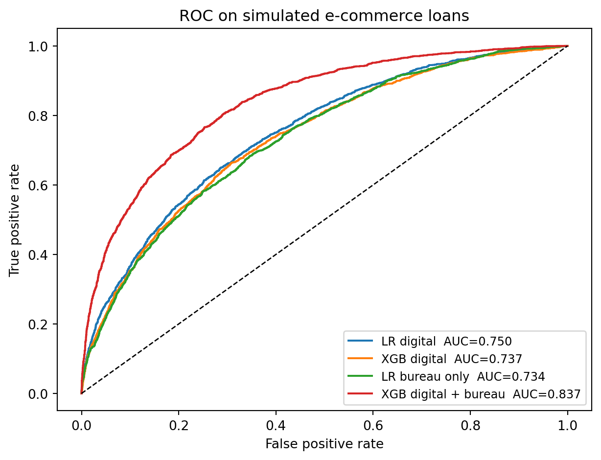
#| fig-cap: "ROC curves on the held-out 30% test set. Digital footprints alone are competitive with a bureau score alone, and the union dominates both."
fig, ax = plt.subplots(figsize=(6.5, 5))
curves = {
    "LR digital":            lr_dig.predict_proba(Xte_dig)[:, 1],
    "XGB digital":           xgb_dig.predict_proba(Xte_dig)[:, 1],
    "LR bureau only":        lr_bur.predict_proba(b_te)[:, 1],
    "XGB digital + bureau":  xgb_cmb.predict_proba(Xte_cmb)[:, 1],
}
for name, sc in curves.items():
    fpr, tpr, _ = roc_curve(yte, sc)
    auc = roc_auc_score(yte, sc)
    ax.plot(fpr, tpr, label=f"{name}  AUC={auc:.3f}")
ax.plot([0, 1], [0, 1], "k--", lw=1)
ax.set_xlabel("False positive rate")
ax.set_ylabel("True positive rate")
ax.set_title("ROC on simulated e-commerce loans")
ax.legend(loc="lower right", fontsize=9)
plt.tight_layout()
plt.show()
```
As shown in @fig-roc, the curves confirm the table. The union classifier's ROC sits strictly above the bureau-only ROC at nearly every operating point, including the low-false-positive region, which is where most lending decisions happen.
### Lift within bureau-safe and bureau-risky buckets
Berg et al.'s cleanest secondary finding is that digital footprints refine the bureau's own classifications. Applicants the bureau rates as safe split into two groups under the digital footprint, and the split is large.
```{python}
#| label: fig-lift-by-bureau
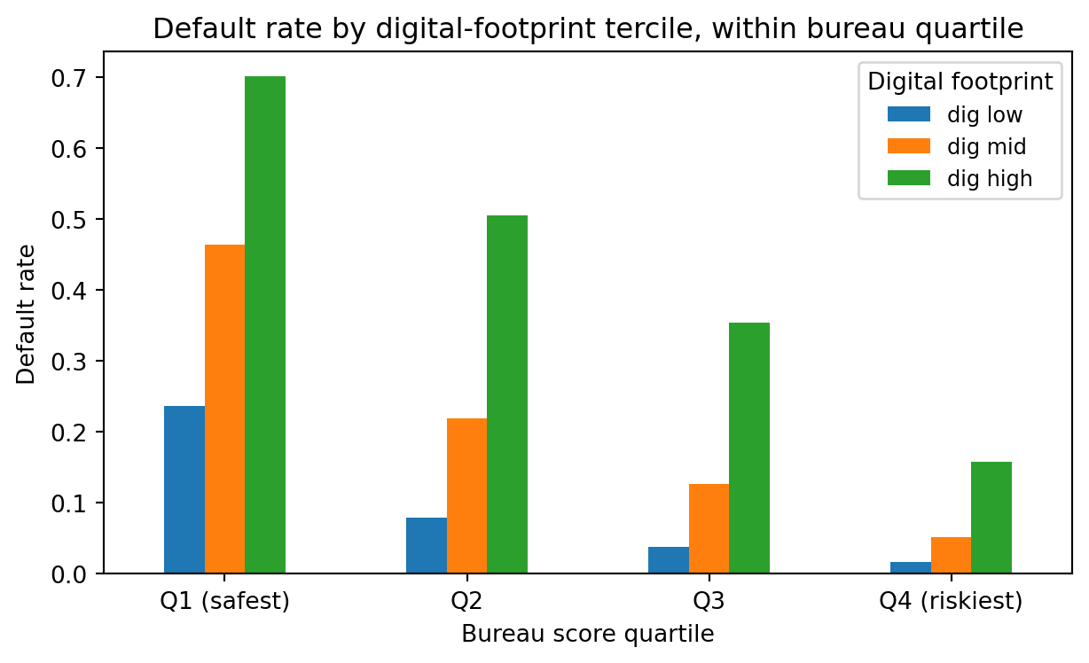
#| fig-cap: "Default rate by digital-footprint risk bucket within each bureau-score quartile. The footprint identifies high-risk borrowers even inside the bureau's 'safest' quartile."
test_df = test_df.copy()
test_df["p_dig"] = xgb_dig.predict_proba(Xte_dig)[:, 1]
test_df["bureau_q"] = pd.qcut(test_df["bureau"], 4,
                               labels=["Q1 (safest)", "Q2", "Q3", "Q4 (riskiest)"])
test_df["dig_q"] = pd.qcut(test_df["p_dig"], 3,
                            labels=["dig low", "dig mid", "dig high"])
rate = (test_df.groupby(["bureau_q", "dig_q"])["y"]
               .mean().unstack("dig_q"))
fig, ax = plt.subplots(figsize=(6.5, 4))
rate.plot(kind="bar", ax=ax)
ax.set_ylabel("Default rate")
ax.set_xlabel("Bureau score quartile")
ax.set_title("Default rate by digital-footprint tercile, within bureau quartile")
ax.legend(title="Digital footprint", fontsize=9)
plt.xticks(rotation=0)
plt.tight_layout()
plt.show()
rate.round(3)
```
As shown in @fig-lift-by-bureau, inside the safest bureau quartile, the highest-risk digital-footprint tercile defaults at a materially higher rate than the lowest tercile. That is where the marginal value lives: on applicants the bureau labels "safe", the digital footprint identifies a non-trivial slice who are not.
### Explainability with SHAP
Global importance from TreeSHAP [@lundberg2017unified, @lundberg2020treeshap] confirms that the model weighted the right features. Because the packaged `shap` library occasionally lags behind XGBoost's binary format, we call the booster's native SHAP contributions directly through `predict(..., pred_contribs=True)`, which returns per-feature Shapley decompositions that sum (plus a bias column) to the log-odds margin.
```{python}
#| label: fig-shap
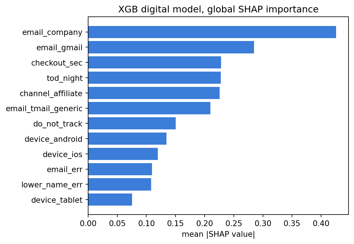
#| fig-cap: "Global mean absolute SHAP attribution per feature on the XGB digital-only model. Email provider dominates, with late-night checkouts and the affiliate channel next."
booster = xgb_dig.get_booster()
dmat = xgb.DMatrix(Xte_dig[:3000], feature_names=feat_names)
contribs = booster.predict(dmat, pred_contribs=True)  # (n, d+1)
shap_vals = contribs[:, :-1]
mean_abs = np.abs(shap_vals).mean(axis=0)
order = np.argsort(mean_abs)[::-1]
top = 12
fig, ax = plt.subplots(figsize=(6.5, 4.5))
ax.barh([feat_names[i] for i in order[:top]][::-1],
        mean_abs[order[:top]][::-1], color="#3b7dd8")
ax.set_xlabel("mean |SHAP value|")
ax.set_title("XGB digital model, global SHAP importance")
plt.tight_layout()
plt.show()
```
As shown in @fig-shap, the ordering matches the generative truth. The three most important features are email-provider indicators, followed by time-of-day, channel, and the typographic flags. Check-out seconds is the most important continuous field. Device flags carry non-trivial weight, especially iOS and Android.
## Device, browser, OS, and email
### Email is not a harmless text field
Berg et al. find that the email host is, individually, the single strongest digital footprint. Why would a free-email domain predict default? The answer is sorting. Corporate email is endogenous to employment: having a corporate address means having a job that issues corporate email, which means regular income, which means a low base-rate default hazard. T-Online (Deutsche Telekom's paid-ISP address) is endogenous to older middle-class customers who paid for a provider address back when that was the norm. Gmail is endogenous to a broader cohort. Yahoo and Hotmail addresses, often created in the early 2000s and held passively, correlate with demographic segments that default at higher rates.
None of this reflects causation. An applicant who switches from a Yahoo address to a Gmail address does not, by that act, become a better credit risk. The email domain is a lagging indicator of lifestyle, not a lever. Regulators and ethicists should treat email-provider effects as proxy effects in the sense of @barocas2016big: a feature whose predictive power arises through correlation with protected or semi-protected attributes.
The local part of the email also carries signal. Formal local parts (first.last, first_last, initials) correlate with formal self-presentation, which correlates with conscientiousness, which correlates with repayment [@klinger2013enterprising]. Local parts containing birth years fix the applicant's age, and age is a strong predictor (though for ECOA-covered loans in the United States, age is a protected basis and may not enter the model directly). Numeric strings, particularly sequential digits, are associated with hastily created, low-friction accounts, which correlate with one-time use and transient behavior.
### Device and operating system
Device type is a sorting signal on income and sophistication. In most OECD countries iOS users have higher mean income than Android users [@demirguc2022global]. Tablets are over-represented in older cohorts and in households with a shared device, both of which carry mild effects on default. Desktop browsers appear more at work or at home, which correlates with income stability. The interaction between device and time-of-day carries extra signal: a phone checkout at 11am is a routine e-commerce session, but a phone checkout at 2am is more likely to be an impulse transaction with an associated higher default hazard.
Fuster, Plosser, Schnabl, and Vickery [@fuster2019role] document a related pattern for mortgages: fintech lenders process applications faster than traditional lenders, and their technology advantage spills over to screening. Digital-footprint fields feed directly into that screening advantage. They are cheap, unforgeable at the margin (the applicant does not know you are reading the user-agent string), and universally available.
Browser, OS, screen resolution, and font set form a device fingerprint that is also useful for fraud detection. Fraud and default are distinct phenomena, but for a typical e-commerce buy-now-pay-later product, fraud shows up as default when the lender tries to collect. Privacy regulation [@gdpr2016, @ccpa2018] treats fingerprinting as personal data even without a stored identifier, which has consequences we return to in @sec-ch17-financial-inclusion-for-thin-file-borrow.
### Channel and traffic source
Traffic channel is quietly one of the most actionable fields. Organic and direct traffic indicate intent: the user sought out the merchant. Paid search indicates intent slightly lower, because some fraction of paid-search traffic is curious rather than converted. Affiliate traffic is the interesting one. Affiliate networks monetize clicks, and their incentive to send any click produces a different mix of applicants than organic. In Berg et al.'s data, affiliate traffic defaults meaningfully more than organic, controlling for other features. The generative process above replicates this via the affiliate-plus-free-provider interaction.
This is a population mixing phenomenon. Affiliates introduce a new subpopulation to the lender, and that subpopulation is not drawn from the same risk distribution as the merchant's direct customers. The digital footprint captures the mix. A lender that ignores channel ignores a structural driver of default.
### Telemetry
Pre-purchase telemetry is the subtlest of the signal families. Seconds spent on the product page, number of pages viewed, inter-click intervals, scroll depth, whether the applicant used autofill, number of validation errors. Each of these is a proxy for care. Care correlates with repayment. Matz, Kosinski, Nave, and Stillwell [@matz2017psychological] show that short digital traces are enough to target communications in personality-congruent ways; the same trace vocabulary works for risk segmentation. Kosinski, Stillwell, and Graepel [@kosinski2013private] demonstrate empirically that basic Facebook likes predict sensitive traits with high accuracy. The same logic extends to checkout-flow telemetry: short, numerous, low-cost signals aggregate into a high-information summary.
Ethics cuts the other way. Telemetry-based scoring is vulnerable to Goodhart's law if surfaced: if applicants know that dwell time on the checkout matters, they will perform dwell time. It is also unusually sensitive to conditions beyond the applicant's control (slow connection, small screen, shared device, disability accommodation), which introduces disparate-impact concerns. We return to this in @sec-ch17-financial-inclusion-for-thin-file-borrow and in the fairness treatment in @sec-ch24.
## Psychometric scoring {#sec-ch17-psychometric}
### Where psychometrics entered credit
Klinger, Khwaja, and del Carpio [@klinger2013enterprising] developed the Entrepreneurial Finance Lab (EFL) score for micro and small-enterprise lending in emerging markets where bureau coverage is sparse and collateral is impossible to pledge. The idea is older than the paper. Psychologists had long claimed that validated personality inventories predict work behaviors, including persistence and conscientiousness. EFL operationalized those inventories for a lending workflow: a 30 to 45 minute tablet-based test of cognitive ability, business skill, and personality, scored against repayment outcomes.
The validation is more convincing than skeptics initially expected. EFL-style scores explain meaningful variation in default beyond observable financial characteristics for thin-file SMEs in Latin America and Africa [@klinger2013enterprising]. The mechanism is orderly: conscientiousness and honesty traits predict repayment behavior; cognitive tests predict business quality; fluid-intelligence subtests predict ability to adapt to shocks. Lenders combine these with whatever observable features they have (prior cash flows, invoices, tax receipts if any) for an extended score.
Two operator-style companies emerged. Lenddo, founded in 2011, built a consumer-side scoring product in Southeast Asia and Latin America that combined smartphone-derived behavioral signals with short psychometric questionnaires. LenddoEFL, after merging with EFL in 2017, positioned the combined offering as a financial-inclusion scoring stack. Tala, a direct lender operating in Kenya, the Philippines, Mexico, and India, built its internal score on phone-derived features (contact list structure, app inventory, SMS metadata, geolocation patterns) combined with lightweight in-app psychometric prompts. All three, at different points, reported AUCs on underserved populations that exceed what any bureau score could provide in those markets, since no bureau score exists for the relevant segment.
The evidence that behavior encoded by a mobile phone is predictive of repayment is not anecdotal. Bjorkegren and Grissen [@bjorkegren2020behavior] use call-detail records from a Caribbean country to predict default on a sample of borrowers, and find AUCs comparable to bureau-level discrimination. Agarwal, Alok, Ghosh, and Gupta [@agarwal2020fintech] show that an Indian fintech's alternative-data score materially improves credit access for millennials and thin-file consumers.
### Psychometric model spirit
A typical psychometric instrument proceeds in three steps.
1. Item bank. A library of $K$ items, each scored on a Likert scale or a forced-choice scale. Items are designed to tap validated psychological constructs (conscientiousness, stress tolerance, fluid intelligence, honesty-humility, locus of control).
2. Latent trait scoring. Classical test theory or item response theory recovers a vector of latent traits $\theta_i \in \mathbb{R}^T$ for each applicant. Under a two-parameter logistic IRT model, the probability that applicant $i$ endorses item $k$ is $\Pr(U_{ik} = 1 \mid \theta_i) = \sigma(a_k (\theta_i - b_k))$, with item discrimination $a_k$ and difficulty $b_k$ estimated from a calibration sample.
3. Risk regression. Traits $\theta_i$ are fed into a downstream default model, possibly alongside observable financial features.
Mathematically, the difference from a standard scorecard is the latent-variable measurement step. Because $\theta_i$ is unobserved, its estimation injects noise: an applicant's measured trait $\hat\theta_i$ is a noisy estimate of the true trait, and the risk regression must account for the measurement error. In practice, commercial systems treat $\hat\theta_i$ as if observed and absorb the measurement noise into a slight reduction in measured predictive power. Rona-Tas [@rona2020predicting] warns against over-reading these systems: a high correlation between a psychometric score and default does not imply that the underlying psychological construct is stable, and small changes to the item bank can meaningfully move the distribution of scores.
### Validity concerns
Three concerns recur.
First, construct validity. An item bank calibrated on one population (say, Colombian micro-entrepreneurs) may not measure the same latent trait in another (Filipino gig workers). Invariance tests from the psychometrics literature rarely make it into production credit-scoring deployments, which means the latent trait can shift meaning across segments without the lender noticing.
Second, gameability. Any psychometric test in a consequential setting is gameable once applicants learn the stakes. EFL and LenddoEFL used forced-choice items with ipsative scoring to attenuate social-desirability bias, but no ipsative design survives a dedicated coaching industry. In markets where a single test opens access to credit, coaching industries emerge within months.
Third, fairness. A psychometric instrument can be a more defensible feature set than a pure correlational feature like email provider, because the items have face validity ("I always pay my bills on time" reads as relevant to credit on its face). But the statistical effects still reflect underlying correlations with education, language, and culture. The bias can show up in test content (cognitive items that advantage test-takers with formal schooling), in item response patterns (extreme-response style varying by culture), or in downstream regression weights (traits that happen to correlate with geography). Fairlearn- and Aequitas-style audits on psychometric-score deployments are rare in the published literature, and we should infer from absence that the audits are not happening at the level they should.
### When psychometric scoring is useful
Psychometric scoring pays off when the bureau is empty, the collateral channel is closed, and the alternative to a psychometric score is no score at all. For micro-enterprise lending in countries with weak credit registries, for migrant-worker remittance-collateralized lending, and for young adults in first-time credit, psychometric plus behavioral scoring is a lifeline. For prime consumer lending in a country with deep bureaus, the marginal AUC gain over a modern fintech stack is small, and the regulatory and operational cost is real. Fit the tool to the gap. Jagtiani and Lemieux [@jagtiani2019roles] and Cornelli et al. [@cornelli2023fintech] show, across jurisdictions, that alternative-data scoring grows fastest exactly where traditional credit infrastructure is thinnest.
## Financial inclusion for thin-file borrowers {#sec-ch17-financial-inclusion-for-thin-file-borrow}
### The inclusion case
Roughly a quarter of adults worldwide have no transaction account at a formal financial institution [@demirguc2022global]. A larger share have accounts but thin credit records. For this population, traditional scoring is either uninformative or unavailable, and loan pricing defaults to worst-case. Alternative data (digital footprints, phone telemetry, psychometrics, transaction flows from mobile money, utility payment history) moves the needle.
Two BIS/IMF working papers frame the empirical case. @bazarbash2019fintech surveys the applications of machine learning and alternative data to credit risk in financial-inclusion settings. The conclusion is conservative but positive: alternative data adds discriminatory power, more for unbanked than for prime, and the measurement gain is largest in markets where the bureau is thin. @bis2020data (a BIS working paper of Gambacorta and coauthors) frames the mechanism as "data versus collateral": fintech lenders use rich transactional data as a substitute for traditional collateral, extending credit to SMEs who could not pledge physical assets. Their panel of Chinese fintech-loan performance, matched to bank-loan performance, shows that the data-driven approach sustains lower default rates at comparable volumes.
@gambacorta2024data extends the analysis to a Chinese fintech lender's individual-consumer panel. Machine-learning models combining traditional data with non-traditional data (app usage, e-commerce activity, social-network signals, travel-pattern data where legally available) materially improve both discrimination and early-warning detection, relative to a bureau-only baseline. The paper's replication of Berg et al.'s signal ordering is notable: non-traditional categorical features dominate, and interactions between traditional and non-traditional features drive the marginal lift. On the fairness side, their analysis suggests that the gains are concentrated in thin-file and rural applicants, which is the inclusion story told numerically.
@lu2023profit goes further and decomposes the alternative-data bundle into its constituents on a 5,214-applicant microloan panel from an Asian lender, covering conventional features, online-shopping records, mobile-phone activity (call logs, app usage, GPS trajectories), and microblog social-media signals. The headline decomposition is that smartphone activity is the dominant layer: profiling with mobile features is roughly 1.3 times more effective than social-media features at improving inclusion (23.05 percent versus 18.11 percent of previously rejected but creditworthy applicants) and 1.3 times more effective at lifting profitability (42 percent versus 33 percent). The ordering matters for this chapter's taxonomy. Mobile telemetry (what @lu2023profit call $F_m$) sits closest to the device and temporal signals formalized in @eq-footprint-vector, whereas microblog sentiment and follower-graph features ($F_s$) are further from the session and therefore cheaper to collect but thinner per unit of predictive lift. Their permutation-importance ranking puts game-app frequency, game-card top-up amount, and office-area GPS visits above the standard economic-capacity features (city disposable personal income, monthly income band), echoing the "ten pixels" result of @berg2020rise in a non-Western setting.
### A back-of-the-envelope inclusion simulation
Let us push the simulated dataset further. Suppose the lender receives a mix of thick-file applicants (with bureau scores) and thin-file applicants (bureau is missing or default-scored to the population mean). How much of the AUC gap does a digital footprint close?
```{python}
#| label: thin-file
df_thin = df.copy()
thin_mask = df_thin.index.isin(
    np.random.default_rng(SEED).choice(df_thin.index, size=int(0.35 * len(df_thin)),
                                       replace=False)
)
df_thin["bureau_obs"] = np.where(thin_mask, np.nan, df_thin["bureau"])
df_thin["bureau_filled"] = np.where(
    thin_mask, df_thin["bureau"].mean(), df_thin["bureau"]
)

train_thin, test_thin = train_test_split(
    df_thin, test_size=0.3, random_state=SEED, stratify=df_thin["y"]
)
ytr_t = train_thin["y"].values
yte_t = test_thin["y"].values
Xtr_cat_t = ohe.transform(train_thin[cat_cols])
Xte_cat_t = ohe.transform(test_thin[cat_cols])
Xtr_dig_t = np.hstack([Xtr_cat_t, train_thin[num_cols].values])
Xte_dig_t = np.hstack([Xte_cat_t, test_thin[num_cols].values])

lr_bur_t = LogisticRegression(max_iter=2000).fit(
    train_thin[["bureau_filled"]].values, ytr_t
)
Xtr_cmb_t = np.hstack([Xtr_dig_t, train_thin[["bureau_filled"]].values])
Xte_cmb_t = np.hstack([Xte_dig_t, test_thin[["bureau_filled"]].values])
xgb_cmb_t = xgb.XGBClassifier(**xgb_params).fit(Xtr_cmb_t, ytr_t)

thin_subset = test_thin["bureau_obs"].isna().values
thick_subset = ~thin_subset

def auc_on(subset, probs):
    return roc_auc_score(yte_t[subset], probs[subset])

p_bur_t = lr_bur_t.predict_proba(test_thin[["bureau_filled"]].values)[:, 1]
p_cmb_t = xgb_cmb_t.predict_proba(Xte_cmb_t)[:, 1]
p_dig_t = xgb.XGBClassifier(**xgb_params).fit(Xtr_dig_t, ytr_t).predict_proba(Xte_dig_t)[:, 1]

pd.DataFrame({
    "subset": ["Thin-file", "Thick-file", "Overall"],
    "Bureau (imputed) AUC": [auc_on(thin_subset, p_bur_t),
                              auc_on(thick_subset, p_bur_t),
                              roc_auc_score(yte_t, p_bur_t)],
    "Digital AUC":          [auc_on(thin_subset, p_dig_t),
                              auc_on(thick_subset, p_dig_t),
                              roc_auc_score(yte_t, p_dig_t)],
    "Digital + Bureau AUC": [auc_on(thin_subset, p_cmb_t),
                              auc_on(thick_subset, p_cmb_t),
                              roc_auc_score(yte_t, p_cmb_t)],
}).round(3)
```
For thin-file applicants, the bureau score is mean-imputed and uninformative, so bureau-only AUC collapses to near 0.5 on that subset. Digital footprint alone recovers most of the predictive power the lender had on thick-file applicants. The digital plus bureau model sits where digital alone sits on thin-file (the bureau column is a constant and contributes nothing), while reaching the combined ceiling on thick-file. That gap is the inclusion value of alternative data: the distance between 0.5 and 0.72-ish, multiplied by the share of the population that is thin-file, multiplied by the welfare value of moving from credit denial to credit with a calibrated price.
### Financial inclusion is a pricing story, not just a discrimination story
Moving from no score to a score of any quality changes the decision from "deny" to "price". Agarwal et al. [@agarwal2020fintech] document large volume increases in Indian millennial lending when a fintech adds alternative data, not because the fintech replaces a prime lender but because it underwrites applicants the prime lender rejected. The welfare gain is the gap between the rejection outcome and a correctly priced loan, which the applicant repays most of the time. @chen2019fintech finds similar volume effects on U.S. fintech mortgage originations. These are not anomalies, they are the operating mechanism of the whole asset class.
The inclusion gain is not evenly distributed across borrowers. @fuster2022predictably documents that alternative data can simultaneously lift average credit access and redistribute it across demographic groups in ways that are not normatively neutral. A lender that serves thin-file applicants more aggressively may also price them more aggressively in states of bad luck, and the combination can produce large heterogeneity in realized welfare. The fairness chapter revisits this point (@sec-ch24).
## Privacy, consent, and ethical limits {#sec-ch17-privacy}
### The regulatory frontier
The legal perimeter for digital-footprint scoring is not the same in every jurisdiction. The two binding regimes for most global lenders are the EU General Data Protection Regulation [@gdpr2016], the California Consumer Privacy Act [@ccpa2018], and their respective successors and counterparts. In 2024 the EU added the Artificial Intelligence Act [@euaiact2024], which classifies credit-scoring systems as high-risk and imposes a baseline of documentation, testing, and logging.
The GDPR's Article 22 restricts solely automated decisions with significant effects. A fully automated credit decision based on digital-footprint data is exactly the class of processing Article 22 covers. Lenders satisfy the article in one of three ways: (a) by getting explicit informed consent, (b) by establishing that the decision is necessary to a contract requested by the applicant, or (c) under authorization from member-state law. In all three paths, the applicant has the right to human review, to contest the decision, and to understand the logic involved. Satisfying "understand the logic" on a gradient-boosted model trained on 200 digital footprint features is non-trivial; see @sec-ch21 for the explainability stack.
The GDPR's lawful-basis requirement bites at the collection stage. Device fingerprinting, cross-site cookies, and pre-existing telemetry acquired through a third-party data broker all require a lawful basis. "Legitimate interest" (Article 6(1)(f)) is the most common basis claimed for passive behavioral data, but lenders that rely on it must pass a balancing test and document it. The European Data Protection Board has tightened its guidance on this point [@kouki2022edpb].
The CCPA is less prescriptive about model behavior and more about consumer rights: opt-out of sale, right to know, right to delete. It does not prohibit alternative-data scoring but does require transparent disclosure that such data is used and a mechanism to access and correct it. The practical effect on a lender is a data lineage requirement that is often tougher than the underwriting-model documentation.
The EU AI Act layers on top. Credit-scoring systems are listed in Annex III as high-risk. Obligations include risk-management documentation, data-governance requirements (quality, relevance, representativeness), technical documentation, logging, transparency to users, human oversight, accuracy and robustness thresholds, and conformity assessment before deployment. Member states will begin enforcement in 2026. A fintech that trained an XGBoost model on digital footprints without a data-governance trail will need to rebuild its documentation, not retrain its model.
### Consent architectures
Consent under the GDPR must be freely given, specific, informed, and unambiguous. A blanket consent to "improve our services" at account creation does not cover a downstream digital-footprint score unless the purpose is specified. The practical architectures that have survived regulator scrutiny tend to share three features.
1. Layered consent. The applicant sees a short primary notice at the point of decision (application form, installment checkout) describing what is collected and why. A deeper layer offers the full data policy. Both must be accessible before submission.
2. Granular toggle for non-essential signals. Passive telemetry that is not strictly necessary for the credit decision (behavioral analytics, cross-site tracking, third-party enrichment) is toggleable. The applicant can opt out without losing access to the core product.
3. Documentation of purpose limitation. Data collected for underwriting cannot be reused for marketing without a separate consent action. The model of consent is a contract-by-contract record, not a one-time blanket.
For U.S. credit decisions covered by ECOA and FCRA, adverse-action notices must identify the primary reasons for denial [@cfpb2017bureau]. A denial driven by digital footprints must be reducible to a short list of intelligible reason codes, which places an explainability floor on the model. SHAP-style explanations can feed the reason-code pipeline, but the reason codes must be recognizable to a consumer: "your application timing was unusual" is not a recognizable reason, "your application was incomplete in ways that predicted repayment difficulty" is borderline, and in practice lenders avoid anything that reads as a dark-pattern disclosure.
### Ethical limits and the proxy problem
Privacy law is the floor. Ethics is the ceiling. Three constraints apply even when compliance is clear.
First, proxies for protected classes. Email provider, device type, and channel are not protected attributes under ECOA, but each correlates with age, gender, income, and in some markets race. @barocas2016big labels this the proxy problem, and @bartlett2022consumer documents its empirical bite in U.S. fintech mortgages. A model that uses these features must be audited for disparate impact (@sec-ch24). If the audit shows that the digital-footprint features carry disparate-impact effects that a lender cannot justify as job-related and consistent with business necessity, the lender's choices are: drop the feature, reweigh the model, or change the decision threshold. "Drop the feature" is not a free lunch because dropping a correlated feature often shifts the weight onto another correlated feature. Fuster et al. [@fuster2022predictably] show that sophisticated models redistribute predictive weight in ways that are not neutral across demographic groups, which the lender must track.
Second, data minimization. The GDPR embeds a data-minimization principle: collect only data adequate, relevant, and limited to what is necessary for the purpose. A lender that collects 500 features but uses 30 in the score is open to a challenge that the other 470 features are collected without a lawful basis. Operational teams routinely ignore this until an audit forces the conversation. The mitigation is to pin feature provenance and model input schema to the same governance object, so data that is not input to the model is not collected on the applicant-underwriting surface.
Third, purpose drift. A model trained for underwriting may be asked, later, to score a customer for cross-selling, pricing renegotiation, or collections triage. Each of those is a new purpose in the GDPR sense and requires either new consent or a new lawful basis. Fintechs run into this when they re-use the underwriting model on a portfolio-level marketing decision without refreshing the consent. The regulatory fix is straightforward. The operational discipline is harder.
### The fairness-privacy tradeoff
Privacy regulation can conflict with fairness regulation. To audit a model for disparate impact, the lender needs to know the protected attribute. In jurisdictions where collecting race is restricted by privacy law (much of the EU, and the UK), the lender does not have the data it needs to run a disparate-impact audit. The Bayesian Improved Surname and Geocoding (BISG) approach, pioneered by the CFPB, imputes race from surname and residence. BISG introduces its own biases, and the imputation error is non-negligible [@hurlin2026fairness]. The inclusion story for digital footprints becomes entangled with the imputation error for race.
The same tension applies to psychometric scoring. To validate a psychometric instrument across demographic groups, one has to know the groups. If the lender cannot collect the grouping variable, it cannot run the validation. The theory of fair credit-scoring assumes a luxury that privacy law does not always grant. Closing this gap is a live research question.
### A scalability note on privacy-preserving computation
For lenders that want to combine data sources without pooling raw records, the cryptographic toolbox has matured enough to be operational. Secure multi-party computation (MPC), federated learning, and differential privacy (DP) each solve a slice of the problem. Federated learning keeps training data on a mobile device and sends only gradients to the central server; it is common in Tala's operating environment where raw phone data cannot leave the device. Differential privacy adds calibrated noise to aggregates to bound disclosure risk; the classic accuracy-privacy frontier is strict but improving. The practical cost is a 2 to 5 percent AUC hit at common DP budgets, which the inclusion economics usually absorbs.
## Scalability and deployment
### From a laptop to production
A digital-footprint scoring stack in production has three distinctive scaling properties. First, most features are categorical with small cardinality (device type, OS family, hour bucket). The feature engineering pipeline is cheaper than in a bureau-feature stack with hundreds of continuous tradeline summaries. Second, the features arrive from different sources at different latencies: device/browser at page load, channel at URL parse, email at form submission, telemetry on keystroke, bureau at API callback. The feature store must stitch these streams by session key. Third, the privacy-regulation overhead is heavy. Every feature must carry a lineage tag identifying its lawful basis and its retention window.
For pandas-scale prototyping (up to a few million rows), a single machine is enough. The simulated dataset above is 30,000 rows and fits in a laptop. For production-scale inference, the decision is between a columnar-store plus classifier-as-a-service architecture (feature store: Feast/DataBricks/Tecton, model server: Triton/TorchServe/MLflow behind FastAPI) and a lighter-weight stack for lenders with smaller volumes.
```{python}
#| label: fastapi-sketch
#| eval: false
# FastAPI stub: accept a JSON session payload, score it, return PD and reason codes.
from fastapi import FastAPI
from pydantic import BaseModel
import numpy as np, joblib, json

app = FastAPI()
artifact = joblib.load("model.joblib")  # dict: model, ohe, cat_cols, num_cols, feat_names

class Session(BaseModel):
    email: str
    device: str
    os: str
    tod: str
    channel: str
    do_not_track: int
    email_err: int
    lower_name_err: int
    checkout_sec: float
    bureau: float

@app.post("/score")
def score(s: Session):
    ohe = artifact["ohe"]
    model = artifact["model"]
    cat = ohe.transform([[getattr(s, c) for c in artifact["cat_cols"]]])
    num = np.array([[getattr(s, n) for n in artifact["num_cols"]]])
    x = np.hstack([cat, num, [[s.bureau]]])
    pd_hat = float(model.predict_proba(x)[0, 1])
    # TreeSHAP reason codes
    import xgboost as xgb
    d = xgb.DMatrix(x, feature_names=artifact["feat_names"])
    contribs = model.get_booster().predict(d, pred_contribs=True)[0, :-1]
    top = np.argsort(-np.abs(contribs))[:3]
    reasons = [artifact["feat_names"][i] for i in top]
    return {"pd": pd_hat, "reason_codes": reasons}
```
The deployment shape for digital-footprint models is the same as any tabular scorer (@sec-ch34). The new surface is the lineage tag and the consent check, and those usually live in the feature store, not in the model server.
### From pandas to Polars, Dask, Spark
The digital-footprint workload at serving time is per-session: one observation at a time, low-latency response. The batch workload at training time can be much larger. A fintech with 10 million applicants and 6 months of telemetry easily exceeds a single-machine pandas frame. Polars beats pandas on memory and speed by a factor of 2 to 10 on typical categorical feature engineering. Dask scales pandas to clusters when the team wants to preserve the pandas API. Spark dominates when the enterprise already runs on Spark. For model training on tens of millions of rows with a few dozen features, distributed XGBoost on Dask or Spark is the standard. For truly massive jobs (hundreds of millions of rows), Spark MLlib or a Spark-XGBoost integration with careful sharding on the categorical encoders is the operational answer.
The overhead that digital footprints introduce is in the streaming join: session-keyed merge of device/browser events with form-submission events with third-party enrichment, under late-arrival and out-of-order delivery. Structured Streaming or Flink handles this cleanly; hand-rolled Python does not. We return to this stack in @sec-ch34.
## Regulatory considerations
A concise regulatory map for a digital-footprint scoring system.
- SR 11-7 [@sr117] requires model risk management. Effective challenge means an independent reviewer must be able to reproduce the model, interrogate its assumptions, and stress-test its performance. Digital-footprint models add two challenges: feature provenance (a reviewer must confirm each feature's lawful basis and data path) and conceptual soundness (why does email provider correlate with default). The second is easier for a psychometric score with face-valid items than for a pure digital footprint with correlational signals.
- Basel II/III and IRB [@basel2006international, @basel2017finalising, @eba2022irb]. For banks using the IRB approach, any rating system (including a digital-footprint component) must be validated, documented, and back-tested. The IRB use test requires that the rating actually drive credit decisions, not sit alongside them. Alternative-data ratings that are advisory only do not count toward IRB capital relief.
- ECOA and FCRA in the United States. The Equal Credit Opportunity Act prohibits discrimination on prohibited bases. Adverse-action notices must list specific reasons [@cfpb2017bureau]. FCRA governs consumer reports, which digital footprints may or may not constitute depending on how the data is assembled and sold. A lender that uses only first-party data (collected directly from the applicant on its site) avoids FCRA's furnisher obligations, but third-party enrichment (device-risk scores from a vendor, email-hygiene APIs) often triggers FCRA.
- GDPR Article 22 and EU AI Act [@gdpr2016, @euaiact2024]. Automated decisions with significant effects require human review, contestability, and explanation. The AI Act adds structured risk-management and logging obligations for high-risk systems, which credit-scoring systems are.
- GDPR purpose limitation and data minimization. The data used in the model must be traceable to a lawful basis, limited to the underwriting purpose, and retained no longer than necessary.
- Fairness and disparate impact. Even where protected-attribute collection is restricted, lenders are responsible for disparate-impact outcomes. An audit pipeline that imputes protected attributes and tests the model on the imputed labels is the bare minimum; the CFPB has been explicit that "we did not collect race" is not a defense.
## Vietnam and emerging markets
### Market context
Vietnam reached about 70 million smartphone users by the mid-2020s, driven by low-cost Android devices and near-universal 4G coverage [@adb2022vnfin]. Three super-apps dominate the consumer digital stack. Zalo, operated by VNG, is the leading domestic messaging and mini-app platform. MoMo is the largest e-wallet by active users. VNPay anchors the banking-QR rail interconnected through NAPAS, the national payment switch [@napas2023report]. Shopee and Lazada are the largest marketplaces, with buy-now-pay-later products (SPayLater, Kredivo) embedded at checkout. Together these platforms generate the digital exhaust that the @berg2020rise framework feeds on: device type, OS version, channel, session timing, payment-rail preferences, QR scans, topup cadence, mini-app usage, and geolocated merchant context.
The bureau side is thinner. CIC covers regulated institutions; private bureau PCB adds supplementary records. Many consumer lenders, including finance companies regulated under SBV Circular 43/2016/TT-NHNN on consumer lending by finance companies, underwrite segments with sparse CIC histories. The @worldbank2021findex 56 percent formal-account figure for 2021 understates today's digital-payments penetration, but it correctly signals that a large slice of the credit-eligible population is thin-file for traditional scoring. Personal-data processing now sits under Decree 13/2023 [@vn_decree13_2023], which imposes consent, data-subject rights, and cross-border transfer controls broadly aligned with GDPR principles.
### Application considerations
A digital-footprint pipeline in Vietnam inherits the structure of @sec-ch17-berg-et-al-2020-on-a-simulated-dataset but changes the feature inventory. Device features reward careful handling of Android fragmentation: brand and price-tier buckets (low, mid, flagship) carry more signal than raw model strings, because the price tier proxies income. Email provider buckets require local additions: Yahoo and Hotmail still appear at non-trivial rates alongside Gmail. Channel features should include Zalo mini-app referrers, Facebook in-app browser detection, and UTM tags from affiliate networks (ACCESSTRADE, Masoffer). Temporal features should encode Tet windows explicitly; a checkout at 02:00 on the third day of Tet is not the same observation as a checkout at 02:00 in July.
E-wallet and QR signals, where a lender has partnered with MoMo, ZaloPay, or VNPay, materially improve thin-file discrimination. Features include wallet tenure, monthly topup count, bill-payment recurrence, P2P transfer centrality, and merchant-category entropy. These features are analogs of the @berg2020rise signal set but richer because the lender observes settled payments rather than clickstream alone. Consent for these features must be traceable under Decree 13/2023, and cross-platform joins typically run through NAPAS Alias or bank-issued tokens rather than raw PII.
### Rationalization
Two arguments transfer the @berg2020rise finding to Vietnam despite the absence of a peer-reviewed replication. First, the mechanism is information-theoretic. Every digital signal Berg et al. exploit has a Vietnamese analog of equal or greater informational density: Android-tier versus iOS is as separating in Vietnam as it is in Germany, and Tet-adjusted hour-of-day is at least as separating as local hour of day in Berg's sample. Second, adjacent-market evidence is consistent. @bjorkegren2020behavior document mobile-metadata repayment signals in an emerging Caribbean market. @gambacorta2024data and @huang2020fintech show platform-data lifts on Chinese panels that resemble Vietnamese BigTech stacks structurally. @bazarbash2019fintech surveys the IMF evidence that alternative data materially extends thin-file frontiers.
The limits matter. Vietnam's Decree 13/2023 restricts profiling that produces legal effects without consent and data-subject rights. Disparate-impact audits are not yet a codified regulatory requirement, but the Personal Data Protection regime treats sensitive-category proxies as high risk, and lenders should audit for proxy effects on ethnicity, migrant status, and province-of-registration.
### Practical notes
An operational recipe for a Vietnamese fintech. First, build the consent ledger under Decree 13/2023 before the feature store. Every feature must carry a provenance tag (first-party, partner-shared, public), a lawful-basis tag, and a retention clock. Second, anchor the feature inventory on the Berg et al. ten, then add wallet features (tenure, topup cadence, bill-pay recurrence) and Zalo/Shopee checkout signals. Bin Android brand and price tier; do not feed raw model strings. Third, stratify evaluation by Tet windows and by province, report AUC and KS uplift over a bureau-only baseline from CIC, and include a thin-file subgroup metric. Fourth, document the pipeline to the standard that SBV Circular 41/2016 validation expects [@sbv_circular41_2016] and align reason-code mappings with the consumer-lending conduct rules under Circular 43/2016/TT-NHNN on consumer lending by finance companies, and reflect the capital adequacy amendments in Circular 22/2023/TT-NHNN (29 Dec 2023) to Circular 41/2016 [@sbv_circular22_2023]. Fifth, for cross-border vendor enrichment (device-risk scores, email hygiene), verify the transfer-impact assessment requirement under Decree 13/2023 before deployment. The IMF Vietnam Article IV reports and the ADB financial-sector work provide the broader macroprudential framing [@imf2024vietnamart4, @adb2022vnfin, @imf2023vietnamart4].
## Takeaways
- Ten digital footprint variables (device, OS, email provider, channel, time-of-day, do-not-track, a few typographic flags, checkout speed) match or beat a bureau score on discriminatory power in an e-commerce loan setting. @berg2020rise document this on real data; the chapter replicates it on a calibrated simulation.
- The predictive content is information-theoretic. Each feature carries modest IV individually, but the stack reaches AUC close to bureau alone. Combining digital plus bureau delivers a large and stable lift above either alone.
- Psychometric and behavioral scoring (EFL, Lenddo, Tala) extend the alternative-data approach to markets where the bureau is empty. The inclusion gain is real and concentrated in thin-file applicants. The validity and fairness caveats are material and should be audited explicitly.
- Privacy regulation (GDPR, CCPA, EU AI Act) sets a floor. Ethics sets a ceiling. The hardest operational problem is proxy effects: features that correlate with protected classes without being protected themselves. Auditing for disparate impact is not optional.
- In production, the digital-footprint pipeline's novel load is not the model, it is the session-keyed streaming join and the per-feature consent and retention metadata.
## Further reading
- @berg2020rise for the empirical anchor of the chapter.
- @bjorkegren2020behavior for mobile-phone metadata as a predictor of repayment.
- @gambacorta2024data and @bis2020data for the Chinese fintech evidence on data versus collateral.
- @bazarbash2019fintech for the IMF survey of alternative data and financial inclusion.
- @klinger2013enterprising for the original EFL psychometric scoring evidence.
- @kosinski2013private and @matz2017psychological for the psychological-profiling-from-digital-traces literature.
- @agarwal2020fintech for fintech alternative data and millennial credit access.
- @fuster2019role and @fuster2022predictably for machine learning in U.S. lending and its distributional consequences.
- @acquisti2016economics for the economics of privacy.
- @acquisti2015privacy on the behavioral economics of privacy decisions, the standard reference for why disclosure choices fail to map cleanly onto stated preferences.
- @goldfarb2011privacy and @miller2018privacy for empirical effects of privacy regulation.
- @aridor2024gdpr and @johnson2023privacy on staggered GDPR rollout and its causal effects on the data industry; the closest natural experiment to a digital-footprint regime change, with cohort-level identification of compliance vintages.
- @janakiraman2018breach and @martin2017privacy on the customer- and firm-side consequences of data breaches and privacy violations, with cohort-event-study designs that complement the digital-footprint pipeline's privacy and consent metadata.
- @turjeman2024databreach for *temporal causal forests* applied to a data breach: signup-vintage-matched cohorts plus heterogeneous behavioral responses (search, message, photo deletion). The methodological template for measuring breach or consent-policy-change effects on a digital-footprint scoring portfolio.
- @bleier2020privacy for the marketing-side review of consumer-privacy research, with implications for the consent and proxy-effect questions raised here.
- @gdpr2016, @ccpa2018, and @euaiact2024 for the regulatory perimeter.
- @cornelli2023fintech for the cross-country growth of digital and big-tech credit.
- @barocas2016big for the proxy problem in data-driven decision systems.