---
execute:
echo: true
eval: true
bibliography: [../references.bib, ../refs/ch-28.bib]
---
# Causal Inference in Credit Scoring {#sec-ch28}
::: {.callout-note appearance="simple" icon="false"}
**Scope: both retail and corporate.** Causal estimands (ATE, CATE, IV, RDD) for credit decisions. Methodology is portfolio-agnostic; worked examples lean retail (account opening, pricing experiments).
:::
## Overview {.unnumbered}
A scorecard is a prediction machine. A credit policy is a causal intervention. Confusing the two is the most common, most expensive mistake in credit analytics. A model that predicts who will default conditional on a bank's existing mix of marketing, pricing, and approval rules is not the same object as a model that tells the bank what happens to defaults if the cutoff moves by ten points, if an auto-decisioning engine replaces human underwriters, or if a new disclosure rule takes effect in California but not in Arizona. The first object is a conditional expectation. The second is a counterfactual.
This chapter walks through the toolkit that credit teams need when the question stops being "what is the probability of default for this applicant" and starts being "what is the effect of this decision on outcomes we care about." Selection bias and feedback loops from the acceptance rule (@sec-ch10) motivate every identification strategy that follows. The chapter covers instrumental variables (@sec-ch28-iv) [@angrist1996identification, @imbens1994identification], difference-in-differences (@sec-ch28-did) [@card1994minimum, @bertrand2004howmuch], regression discontinuity at score cutoffs (@sec-ch28-rdd) [@hahn2001identification, @imbens2008recent, @lee2010regression], and double machine learning (@sec-ch28-dml) for high-dimensional controls [@chernozhukov2018double, @belloni2014inference]. It closes with a practical protocol for causal validation of a deployed model: how to distinguish covariate drift from a genuine policy shift, and how to retrain without amplifying feedback bias.
### Notation {.unnumbered}
Let $Y \in \{0, 1\}$ be the observed default indicator, $D \in \{0, 1\}$ a binary treatment (a loan, a policy, a product), $X \in \mathbb{R}^p$ a vector of pre-treatment covariates, and $Z$ an instrument. Following @rubin1974estimating and @holland1986statistics, potential outcomes are written $Y(1), Y(0)$, with $Y = D Y(1) + (1 - D) Y(0)$. The average treatment effect is $\tau = \mathbb{E}[Y(1) - Y(0)]$. The conditional average treatment effect (CATE) is $\tau(x) = \mathbb{E}[Y(1) - Y(0) \mid X = x]$. The local average treatment effect (LATE) is $\tau_{\text{LATE}} = \mathbb{E}[Y(1) - Y(0) \mid \text{compliers}]$. Expectations are over the population unless indexed otherwise. All code uses fixed seeds.
## Why causality matters in credit {#sec-ch28-causal}
A scorecard trained on accepted applicants estimates $\Pr(Y = 1 \mid X, D = 1)$, the probability of default given covariates and acceptance. A lender usually does not want this quantity. It wants $\Pr(Y(1) = 1 \mid X)$, the probability an applicant would default if extended credit, including the applicants the bank currently rejects. Under random assignment of $D$, the two quantities coincide. Under any non-random acceptance rule, they do not. That gap is the entire point of this chapter.
The gap matters for three practical reasons. First, policy decisions are counterfactual. When a chief risk officer asks "what happens if we lower the approval cutoff by twenty points," the answer is not a conditional expectation computed on the current training data. It is a counterfactual prediction that requires the CRO to reason about a distribution the current scorecard has never seen. Second, feedback loops compound. The next training cycle inherits the current acceptance rule through the observed label set, so any bias is baked into the next vintage [@heckman1979sample]. Third, regulation is increasingly causal. SR 11-7 model risk guidance and the EU AI Act both ask for evidence that a model behaves sensibly under intervention, not only under repeated sampling from the operating distribution.
Predictive inference and causal inference share a lot of machinery. Both use regression, both use cross-validation, both worry about bias and variance. They diverge on the target estimand and the identification assumptions. A scorecard's target is an optimal ranker under the observed joint distribution; its identification assumption is iid sampling. A causal estimator's target is a counterfactual contrast; its identification assumption is some form of unconfoundedness, exogeneity, or quasi-randomization. Confusing the two produces confident point estimates that collapse the moment the intervention is actually tried.
Emerging markets sharpen the stakes. When the State Bank of Vietnam imposes a system-wide credit growth ceiling (the so-called credit-room tool) or caps nominal lending rates, every bank faces a policy intervention whose effect on default cannot be read off a scorecard. The identification problem is bigger than in the US because the instruments are coarser, the data are thinner, and the counterfactual is a year in which the policy did not exist. A credit team in Hanoi that treats its logistic PD as a causal summary of how an interest-rate cap changes default has already lost the argument with the supervisor [@imf2023vietnamart4, @bis_credit_em2022]. The same causal toolkit, IV for officer assignment, DiD across provinces that bind differently, RDD at supervisory thresholds, DML for rich controls, is what survives the audit.
A small worked example sets up the rest of the chapter.
```{python}
import numpy as np
import pandas as pd
import matplotlib.pyplot as plt
import sys
from pathlib import Path

sys.path.insert(0, '../code')
from creditutils import ks_statistic, gini, stable_sigmoid

rng = np.random.default_rng(7)
n = 20000

# A latent risk score X. Defaulters have lower scores on average.
X = rng.normal(0, 1, size=n)

# True counterfactual default probability under extending credit.
# Monotonically decreasing in X.
p_default = stable_sigmoid(-(2.0 + 1.5 * X))

# Potential outcome: default if extended credit.
Y1 = (rng.uniform(size=n) < p_default).astype(int)

# A bank that approves only the top 40 percent of X values.
cutoff = np.quantile(X, 0.6)
D = (X >= cutoff).astype(int)

# Observed outcome: default realized only for approved accounts.
Y_obs = np.where(D == 1, Y1, np.nan)

approved = pd.DataFrame({
    "X": X[D == 1],
    "Y": Y_obs[D == 1],
})
print(f"Approval rate: {D.mean():.3f}")
print(f"Observed default rate among approved: {approved['Y'].mean():.3f}")
print(f"True population default rate under blanket acceptance: {p_default.mean():.3f}")
```
The observed default rate on the approved book is much lower than the population rate. That is expected: the bank selected the low risk tail of $X$. A naive scorecard estimates a conditional probability on the accepted slice only. Any question of the form "what would the default rate be if we approved more applicants" requires extrapolation to the unselected slice. The rest of this chapter is about how to do that extrapolation honestly.
## Selection bias and feedback loops {#sec-ch28-selection}
### The accepted-only problem
@sec-ch10 laid out reject inference for the static case. The causal framing sharpens the picture. Let $S \in \{0, 1\}$ indicate whether an applicant is observed with a realized outcome. In the simplest bank, $S = D$: only accepted applicants generate $Y$. The training sample is selected on $D = 1$. Suppose the bank runs logistic regression:
$$
\widehat{\Pr}(Y = 1 \mid X, D = 1) = \sigma(X^\top \widehat{\beta}).
$$ {#eq-selected-logit}
Under the potential-outcomes framework, what the bank actually estimates is $\Pr(Y(1) = 1 \mid X, D = 1)$, not $\Pr(Y(1) = 1 \mid X)$. These coincide only if $D \perp Y(1) \mid X$, the ignorability condition [@rosenbaum1983central]. Ignorability fails whenever a loan officer, a rules engine, or a previous scorecard used an unobserved signal correlated with $Y(1)$. The usual suspects are income verification notes, soft inquiries, the phone conversation with the branch, cross-product holdings invisible to the modeling table, and the previous model's residual. Each of these is a back-door path that contaminates the coefficient estimate [@pearl1995causal].
### Feedback amplification
The problem compounds over vintages. Vintage $t$'s model trains on vintage $t - 1$'s accepted book. The acceptance rule at vintage $t$ is a function of that model. Vintage $t + 1$'s training data is the accepted subset of a population screened by vintage $t$'s rule. Biases that produce conservative rejections of a subpopulation in year $t$ make that subpopulation vanish from the data in year $t + 1$, so the next model has nothing to learn about it. A feedback loop does not converge to an unbiased estimator. It converges to a fixed point that depends on the initial bias.
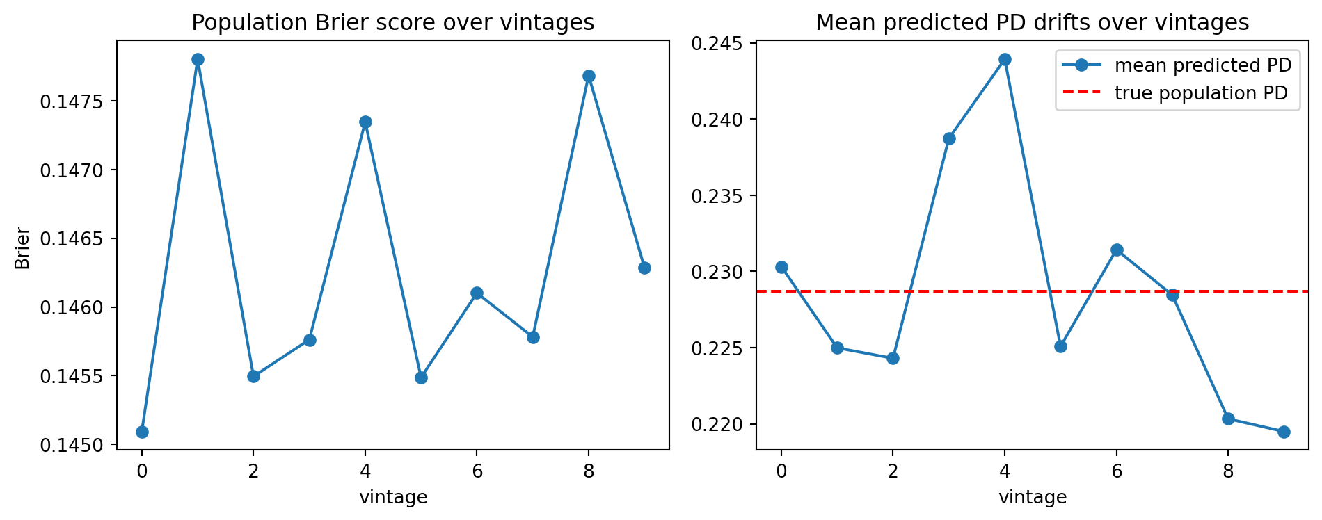
The next simulation makes this concrete. The true generative model is fixed. The bank retrains every quarter on its own accepted book and uses the current model to decide acceptance. Over eight quarters, watch what happens to the out-of-sample calibration error on the unselected population.
```{python}
from sklearn.linear_model import LogisticRegression
from sklearn.metrics import brier_score_loss
from sklearn.preprocessing import StandardScaler

rng = np.random.default_rng(11)
N = 50000
d = 4
true_beta = np.array([-0.8, -0.6, 0.4, 0.3])
true_intercept = -1.5

def simulate_applicants(n, rng):
    return rng.normal(0, 1, size=(n, d))

def true_pd(X):
    lin = true_intercept + X @ true_beta
    return stable_sigmoid(lin)

# Vintage 0: seed by accepting a random 60 percent slice.
X0 = simulate_applicants(N, rng)
p0 = true_pd(X0)
Y0 = (rng.uniform(size=N) < p0).astype(int)
seed_accept = rng.uniform(size=N) < 0.6
X_train = X0[seed_accept]
Y_train = Y0[seed_accept]

scaler = StandardScaler().fit(X_train)
model = LogisticRegression(max_iter=2000).fit(scaler.transform(X_train), Y_train)

calibration_errors = []
pop_pd_hat = []
accept_rates = []
for t in range(10):
    X_new = simulate_applicants(N, rng)
    p_new = true_pd(X_new)
    # Score and accept top 50 percent by predicted PD (safest half).
    s = model.predict_proba(scaler.transform(X_new))[:, 1]
    accept = s <= np.median(s)
    # Realize outcomes only for accepted applicants.
    Y_new = np.where(rng.uniform(size=N) < p_new, 1, 0)
    # Population-level calibration: compare model PD to true PD everywhere.
    pop_brier = brier_score_loss(
        (rng.uniform(size=N) < p_new).astype(int),
        s,
    )
    calibration_errors.append(pop_brier)
    pop_pd_hat.append(s.mean())
    accept_rates.append(accept.mean())
    # Retrain on the accepted book.
    X_train = X_new[accept]
    Y_train = Y_new[accept]
    scaler = StandardScaler().fit(X_train)
    model = LogisticRegression(max_iter=2000).fit(
        scaler.transform(X_train), Y_train
    )

fig, ax = plt.subplots(1, 2, figsize=(10, 4))
ax[0].plot(calibration_errors, marker="o")
ax[0].set_title("Population Brier score over vintages")
ax[0].set_xlabel("vintage")
ax[0].set_ylabel("Brier")
ax[1].plot(pop_pd_hat, marker="o", label="mean predicted PD")
ax[1].axhline(true_pd(simulate_applicants(100000, rng)).mean(),
              color="red", linestyle="--", label="true population PD")
ax[1].legend()
ax[1].set_title("Mean predicted PD drifts over vintages")
ax[1].set_xlabel("vintage")
plt.tight_layout()
plt.show()
```
Two things happen. The mean predicted PD drifts downward because each model trains on a progressively safer book. The Brier score on the full population drifts upward because the model's predictions become less informative outside the region where it still sees data. The drift is not a bug in logistic regression. It is a consequence of feeding the output of the selection rule back into the training loop without correction. Reject inference [@heckman1979sample] (see @sec-ch10) is one fix. The rest of this chapter offers complementary fixes that use randomization or quasi-randomization in the acceptance rule itself.
## Instrumental variables {#sec-ch28-iv}
### Setup and LATE
Instrumental variables (IV) handle endogenous treatment. Let $D$ be a potentially endogenous treatment and $Y$ the outcome. An instrument $Z$ satisfies three conditions [@angrist1996identification]:
1. Relevance: $\operatorname{Cov}(Z, D) \neq 0$.
2. Exclusion: $Z$ affects $Y$ only through $D$.
3. Unconfounded instrument: $Z \perp (Y(0), Y(1), D(0), D(1)) \mid X$.
Under monotonicity, which rules out defiers, @imbens1994identification show that the Wald estimator identifies the local average treatment effect (LATE):
$$
\tau_{\text{LATE}} = \frac{\mathbb{E}[Y \mid Z = 1] - \mathbb{E}[Y \mid Z = 0]}{\mathbb{E}[D \mid Z = 1] - \mathbb{E}[D \mid Z = 0]}
= \mathbb{E}[Y(1) - Y(0) \mid \text{compliers}].
$$ {#eq-late-wald}
The estimand is not the population ATE. It is the ATE restricted to compliers: units whose treatment status is switched by the instrument. In credit, compliers are the subset of applicants whose loan decision would flip if they were assigned to a different loan officer, or whose decision would flip between the auto-decisioning engine and a human underwriter.
### Two worked examples
Two instruments show up repeatedly in credit research. The first is loan officer leniency [@arnold2018racial, @dobbie2021measuring]. Applications are quasi-randomly assigned to officers whose approval tendencies differ. The average approval rate of an applicant's assigned officer, computed on that officer's other cases (leave-one-out), is an instrument for the applicant's own approval. The second is auto-decisioning assignment. A bank that routes marginal applications to an algorithmic engine for some geographies or time windows and to human underwriters elsewhere has, effectively, a randomized assignment of a decision technology. The difference in approval rates between the two arms identifies the causal effect of auto-decisioning conditional on the first-stage wedge.
The simulation below builds a stylized version. Applicants are randomized to loan officers with heterogeneous leniency. Default is a function of a latent risk plus a causal effect of receiving credit.
```{python}
from linearmodels.iv import IV2SLS

rng = np.random.default_rng(3)
n = 20000

# Latent creditworthiness and observed noisy signals.
U = rng.normal(0, 1, size=n)
X1 = U + rng.normal(0, 0.5, size=n)
X2 = 0.5 * U + rng.normal(0, 1, size=n)

# Loan officers: 200 officers, each with a leniency level.
n_officers = 200
officer_leniency = rng.uniform(-0.8, 0.8, size=n_officers)
officer_id = rng.integers(0, n_officers, size=n)
Z = officer_leniency[officer_id]  # leave-one-out leniency instrument

# Treatment: approval decision. Endogenous because it also depends on U.
approval_util = 0.4 * X1 - 0.3 * X2 + 0.7 * U + Z + rng.normal(0, 1, size=n)
D = (approval_util > 0).astype(int)

# Potential outcomes. True causal effect of credit approval on a one-year
# default flag is beta_D = -0.05 (credit access reduces default by stabilizing
# cash flow, say). Endogeneity: U affects Y directly.
beta_D = -0.05
Y = 0.1 - 0.4 * X1 + 0.2 * X2 + 0.5 * U + beta_D * D + rng.normal(0, 0.3, size=n)

df = pd.DataFrame({"Y": Y, "D": D, "X1": X1, "X2": X2, "Z": Z})

# OLS will be biased because D correlates with U via approval_util.
import statsmodels.api as sm
ols = sm.OLS(df["Y"], sm.add_constant(df[["D", "X1", "X2"]])).fit()
print("OLS estimate of effect of D on Y:", round(ols.params["D"], 4))

# 2SLS using officer leniency as instrument.
iv = IV2SLS(
    dependent=df["Y"],
    exog=sm.add_constant(df[["X1", "X2"]]),
    endog=df["D"],
    instruments=df["Z"],
).fit()
print(iv.summary.tables[1])
print(f"\nFirst-stage F statistic: {iv.first_stage.diagnostics.loc['D','f.stat']:.2f}")
```
The OLS coefficient on $D$ is biased toward zero (or even flips sign) because approval is correlated with unobserved creditworthiness $U$, which also reduces $Y$. The 2SLS estimate recovers a number close to the true $\beta_D = -0.05$. The first-stage F statistic, which @stock2002survey and @andrews2019weak recommend as a weak-instrument diagnostic, sits well above the rule-of-thumb 10 threshold.
### Practical guardrails
Three guardrails matter in production use of IV in credit.
First, relevance is testable. Compute the first-stage F. If it is below 10, LATE inference is dominated by weak-instrument bias. The effective F of @andrews2019weak is a more modern alternative.
Second, exclusion is untestable but falsifiable. Use placebo outcomes that should be unaffected by the treatment. If the instrument moves them, the exclusion restriction is suspect. In the loan-officer setting, a common falsification is to regress applicant-observable covariates like age or prior score on officer leniency. If leniency predicts applicant age, assignment was not random.
Third, monotonicity is the least scrutinized assumption. A lenient officer approves everyone a strict officer would, and more. In reality, officers specialize. Some prioritize low-doc self-employed, some prioritize thin-file young borrowers. @angrist1996identification's monotonicity requires that no applicant is a "defier." A useful diagnostic is to partition officers by leniency and check whether approval rates are monotone in leniency across observable applicant strata.
## Difference-in-differences for credit policy {#sec-ch28-did}
### Setup
A credit policy often changes in one place at one time. A state tightens payday loan rules. A bank raises the minimum credit score for a product line in region A but not region B. A regulator imposes an ability-to-pay rule on a subset of lenders. Difference-in-differences (DiD) exploits the two-way structure. Let $i$ index units (zip codes, branches, borrower cohorts) and $t$ index time. Let $G_i \in \{0, 1\}$ indicate treatment group and $T_t \in \{0, 1\}$ indicate post-treatment period. The two-way fixed-effects (TWFE) regression is
$$
Y_{it} = \alpha_i + \gamma_t + \tau G_i T_t + \varepsilon_{it},
$$ {#eq-did-twfe}
and under parallel trends,
$$
\mathbb{E}[Y_{it}(0) \mid G_i = 1, T_t = 1] - \mathbb{E}[Y_{it}(0) \mid G_i = 1, T_t = 0]
=
\mathbb{E}[Y_{it}(0) \mid G_i = 0, T_t = 1] - \mathbb{E}[Y_{it}(0) \mid G_i = 0, T_t = 0],
$$ {#eq-parallel-trends}
the coefficient $\tau$ identifies the average treatment effect on the treated (ATT). The assumption says that, absent treatment, treated and control units would have moved in parallel over the event window. It is not a statement about levels. It is a statement about counterfactual trends.
### Modern DiD caveats
TWFE has known problems under heterogeneous or staggered treatment [@goodmanbacon2021difference, @callaway2021difference, @dechaisemartin2020two, @sunabraham2021estimating, @roth2023what]. When units adopt treatment at different times and the treatment effect varies across units, TWFE is a weighted average with negative weights on some comparisons. The recent literature (Callaway-Sant'Anna, de Chaisemartin-D'Haultfoeuille, Sun-Abraham) develops estimators that avoid this. For a single policy that kicks in at a single date across one group, the classical estimator in @eq-did-twfe still works.
@bertrand2004howmuch's classic paper on DiD standard errors reminds us that inference must cluster at the unit level because unobserved shocks are serially correlated. Cluster-robust variance estimators are the default.
### Simulated policy change
The following simulation builds a natural experiment. A state rolls out a disclosure requirement that forces subprime card issuers to show an annualized cost figure on every statement. The hypothesis is that the disclosure reduces delinquency. Other states keep the old rule. We simulate the default rate in both arms before and after the rollout.
```{python}
rng = np.random.default_rng(17)

n_units = 400             # 400 zip codes
T = 24                    # 24 monthly periods
treat_start = 12          # policy takes effect at month 12
share_treated = 0.5

unit_ids = np.arange(n_units)
treated = (rng.uniform(size=n_units) < share_treated).astype(int)

# Unit-level base default rate.
unit_alpha = rng.normal(0.08, 0.02, size=n_units)
# Common time trend.
time_gamma = 0.001 * np.arange(T) + 0.005 * np.sin(np.arange(T) / 3)
# True treatment effect: reduces default rate by 0.015 after policy rollout.
true_tau = -0.015

rows = []
for i in unit_ids:
    for t in range(T):
        post = int(t >= treat_start)
        eta = rng.normal(0, 0.008)
        y = (
            unit_alpha[i]
            + time_gamma[t]
            + true_tau * treated[i] * post
            + eta
        )
        rows.append({"unit": i, "t": t, "post": post,
                     "treated": treated[i], "y": y})
panel = pd.DataFrame(rows)

# TWFE regression with cluster-robust SE.
import statsmodels.formula.api as smf
model = smf.ols(
    "y ~ treated*post + C(unit) + C(t)",
    data=panel,
).fit(cov_type="cluster", cov_kwds={"groups": panel["unit"]})

interaction = "treated:post"
did_est = model.params[interaction]
did_se = model.bse[interaction]
print(f"DiD estimate: {did_est:.5f}  SE (cluster): {did_se:.5f}")
print(f"True tau: {true_tau:.5f}")
```
The DiD estimate sits within a standard error of the true effect. The next step checks parallel trends in the pre-period, which is the only part of the identification assumption that is testable.
```{python}
pre = panel[panel["t"] < treat_start].copy()
pre["t"] = pre["t"].astype("category")
pretrend = smf.ols(
    "y ~ C(t)*treated + C(unit)", data=pre,
).fit(cov_type="cluster", cov_kwds={"groups": pre["unit"]})

# Inspect the interaction terms. Under parallel trends, they should be near 0.
int_rows = [r for r in pretrend.params.index if ":treated" in r]
print(pretrend.params[int_rows].round(4))
```
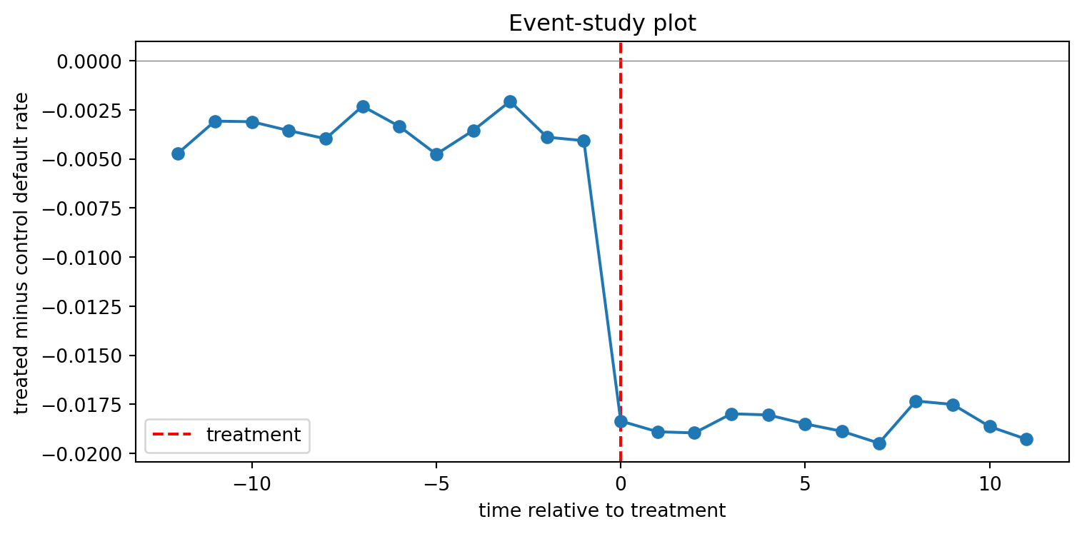
Small and statistically indistinguishable from zero supports parallel trends in the pre-window. An event-study plot makes this visual.
```{python}
event = panel.copy()
event["rel_t"] = event["t"] - treat_start

# Estimate effect at each event time for treated-vs-control.
event_effects = []
for rel in range(-treat_start, T - treat_start):
    sub = event[event["rel_t"] == rel]
    diff = (
        sub.loc[sub["treated"] == 1, "y"].mean()
        - sub.loc[sub["treated"] == 0, "y"].mean()
    )
    event_effects.append({"rel_t": rel, "diff": diff})
ev = pd.DataFrame(event_effects)

plt.figure(figsize=(8, 4))
plt.axvline(0, color="red", linestyle="--", label="treatment")
plt.axhline(0, color="grey", linewidth=0.5)
plt.plot(ev["rel_t"], ev["diff"], marker="o")
plt.xlabel("time relative to treatment")
plt.ylabel("treated minus control default rate")
plt.title("Event-study plot")
plt.legend()
plt.tight_layout()
plt.show()
```
The line sits near zero in the pre-window and drops after the policy kicks in. Visual event-study evidence in support of parallel trends is, in practice, the DiD assumption that regulators and credit committees actually look at.
### When DiD goes wrong in credit
Credit portfolios violate DiD assumptions in several ways. Parallel trends fails when the policy is announced before it takes effect, so issuers adjust lending before the event window. Anticipation effects show up as divergent pre-trends. Selection into treatment fails when treated and control states differ systematically, for example, when the state rolled out the rule precisely because it had high delinquency. Spillovers fail when card issuers in the treated state tighten nationwide underwriting to reduce operational complexity, which contaminates the control arm. Careful papers in credit policy [@agarwal2017regulating, @keys2010did] document how each of these shows up and how to probe it.
## Regression discontinuity at score cutoffs {#sec-ch28-rdd}
### Sharp RDD is natural in credit
Credit is the cleanest laboratory on earth for regression discontinuity. Approval rules typically take the form "approve if score $\geq c$". Around the cutoff, applicants with a score of $c - 1$ and applicants with a score of $c$ are, by every observable and most unobservables, equivalent. Treatment (approval) changes discontinuously at $c$. Outcomes can be compared across the cutoff to estimate the local causal effect of approval.
Formally, let $X$ be the score (running variable) and $D = \mathbb{1}[X \geq c]$. Under the continuity condition of @hahn2001identification,
$$
\mathbb{E}[Y(0) \mid X = x] \text{ and } \mathbb{E}[Y(1) \mid X = x] \text{ are continuous at } x = c,
$$ {#eq-rdd-continuity}
the sharp RDD estimand is
$$
\tau_{\text{RDD}} = \lim_{x \downarrow c} \mathbb{E}[Y \mid X = x] - \lim_{x \uparrow c} \mathbb{E}[Y \mid X = x].
$$ {#eq-rdd-tau}
This is the ATE at the cutoff, for units whose score lands exactly at $c$. The estimand generalizes locally to a small neighborhood under a smoothness assumption.
Estimation uses local linear regression on each side of the cutoff. @imbens2008recent and @lee2010regression lay out the mechanics. @calonico2014robust provide robust bias-corrected inference, which is what practitioners should use in production.
### From-scratch local linear RDD
```{python}
rng = np.random.default_rng(23)
n = 10000
# Running variable: credit bureau score, centered at 0 for convenience.
X = rng.normal(0, 50, size=n)
cutoff = 0.0
D = (X >= cutoff).astype(int)
# True outcome: default rate declines smoothly in X, plus a discontinuous
# effect of approval. Here approval itself causes downstream default because
# borrowers who are approved take on risky debt. True jump is +0.04.
true_jump = 0.04
Y_latent = 0.2 - 0.003 * X + true_jump * D + rng.normal(0, 0.05, size=n)
Y = Y_latent
def local_linear_rdd(X, Y, cutoff, bandwidth, kernel="triangular"):
"""Local linear RDD estimator on each side of cutoff."""
left = X < cutoff
right = X >= cutoff
def kern(u):
if kernel == "triangular":
return np.maximum(1 - np.abs(u), 0)
return (np.abs(u) <= 1).astype(float)
def fit_side(mask):
Xs = X[mask]
Ys = Y[mask]
u = (Xs - cutoff) / bandwidth
w = kern(u)
w = w * (np.abs(u) <= 1)
Xd = np.column_stack([np.ones_like(Xs), Xs - cutoff])
W = np.diag(w)
# WLS closed form.
A = Xd.T @ W @ Xd + 1e-8 * np.eye(2)
beta = np.linalg.solve(A, Xd.T @ W @ Ys)
return beta[0] # intercept at cutoff
mu_left = fit_side(left)
mu_right = fit_side(right)
return mu_right - mu_left
# Imbens-Kalyanaraman rule-of-thumb bandwidth (simplified)
h_iks = 1.06 * X.std() * n ** (-1 / 5)
tau_hat = local_linear_rdd(X, Y, cutoff, h_iks)
print(f"Bandwidth: {h_iks:.2f}")
print(f"RDD estimate: {tau_hat:.4f} (true jump = {true_jump})")
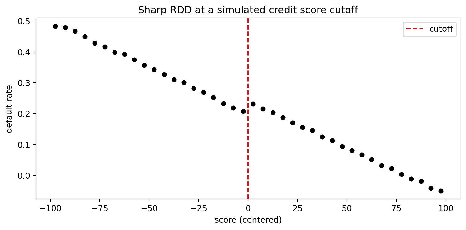
# Plot the binned average outcome around the cutoff.
bins = np.linspace(-100, 100, 41)
mids = (bins[:-1] + bins[1:]) / 2
bucket = np.digitize(X, bins) - 1
valid = (bucket >= 0) & (bucket < len(mids))
agg = pd.DataFrame({"x": mids[bucket[valid]], "y": Y[valid]})
binned = agg.groupby("x")["y"].mean().reset_index()
plt.figure(figsize=(8, 4))
plt.scatter(binned["x"], binned["y"], s=25, color="black")
plt.axvline(0, color="red", linestyle="--", label="cutoff")
plt.xlabel("score (centered)")
plt.ylabel("default rate")
plt.title("Sharp RDD at a simulated credit score cutoff")
plt.legend()
plt.tight_layout()
plt.show()
```
The from-scratch local linear estimator recovers the true jump. The binned scatter shows the discontinuity at zero.
### Robust nonparametric RDD
The package `rdrobust` implements the @calonico2014robust robust bias-corrected confidence intervals. If the package is not installed, fall back on the implementation above.
```{python}
try:
    from rdrobust import rdrobust
    rd = rdrobust(y=Y, x=X, c=cutoff)
    print(rd)
except ImportError:
    print("rdrobust not installed, skipping Calonico-Cattaneo-Titiunik call.")
```
### McCrary density test
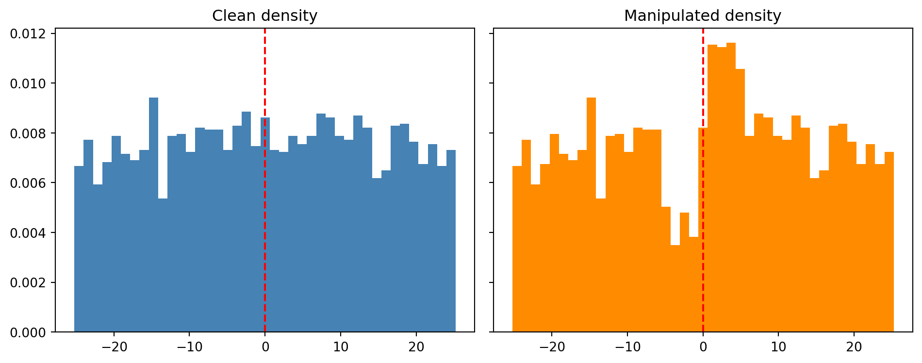
The internal validity of RDD rests on the assumption that units cannot precisely manipulate the running variable around the cutoff. In credit, bureau scores and internal scorecards are not fully in the applicant's control, but loan officers sometimes can nudge scores by re-classifying inputs at the margin. If they do, the density of $X$ will show a jump at the cutoff. @mccrary2008manipulation proposed a local polynomial density test for exactly this. @cattaneo2020simple improved it.
```{python}
def mccrary_density_test(X, cutoff, bw=None, grid=41):
    """Simplified McCrary density test by local polynomial on each side."""
    if bw is None:
        bw = 1.06 * X.std() * len(X) ** (-1/5)
    bins = np.linspace(cutoff - 3 * bw, cutoff + 3 * bw, grid + 1)
    mids = (bins[:-1] + bins[1:]) / 2
    counts, _ = np.histogram(X, bins=bins)
    widths = np.diff(bins)
    density = counts / (len(X) * widths)

    def side_est(mask):
        x = mids[mask]
        y = density[mask]
        u = (x - cutoff) / bw
        w = np.maximum(1 - np.abs(u), 0)
        Xd = np.column_stack([np.ones_like(x), x - cutoff])
        W = np.diag(w)
        beta = np.linalg.solve(Xd.T @ W @ Xd + 1e-9 * np.eye(2),
                                Xd.T @ W @ y)
        return beta[0]
    left = mids < cutoff
    right = mids >= cutoff
    return side_est(right) - side_est(left), mids, density

# Test on the clean data first.
jump_clean, mids_clean, dens_clean = mccrary_density_test(X, 0.0)
print(f"McCrary density jump on clean data: {jump_clean:.5f}")

# Now simulate manipulation: 5 percent of applicants just below the cutoff
# are nudged to just above.
X_manip = X.copy()
below = (X_manip > -5) & (X_manip < 0)
shift = (rng.uniform(size=below.sum()) < 0.5)
X_manip[np.where(below)[0][shift]] = rng.uniform(0, 5, size=shift.sum())
jump_manip, mids_manip, dens_manip = mccrary_density_test(X_manip, 0.0)
print(f"McCrary density jump on manipulated data: {jump_manip:.5f}")

fig, ax = plt.subplots(1, 2, figsize=(10, 4), sharey=True)
ax[0].bar(mids_clean, dens_clean, width=(mids_clean[1] - mids_clean[0]),
         color="steelblue")
ax[0].axvline(0, color="red", linestyle="--")
ax[0].set_title("Clean density")
ax[1].bar(mids_manip, dens_manip, width=(mids_manip[1] - mids_manip[0]),
         color="darkorange")
ax[1].axvline(0, color="red", linestyle="--")
ax[1].set_title("Manipulated density")
plt.tight_layout()
plt.show()
```
The clean density is continuous at zero. The manipulated density shows a deficit just below and a spike just above, exactly the signature @mccrary2008manipulation warned about. In production credit RDD work, always run the density test before trusting the estimated jump.
### Fuzzy RDD when the cutoff is a recommendation
Not every credit cutoff is sharp. Some scorecards feed into a human underwriter who can override. In that case, $D$ does not jump from 0 to 1 at $c$; it jumps from a probability $p_0$ to a probability $p_1 > p_0$. The fuzzy RDD estimand is
$$
\tau_{\text{fuzzy}} = \frac{\lim_{x \downarrow c} \mathbb{E}[Y \mid X = x] - \lim_{x \uparrow c} \mathbb{E}[Y \mid X = x]}
{\lim_{x \downarrow c} \mathbb{E}[D \mid X = x] - \lim_{x \uparrow c} \mathbb{E}[D \mid X = x]}.
$$ {#eq-rdd-fuzzy}
This is a local Wald ratio that identifies LATE at the cutoff under monotonicity, exactly as in the IV framing. Auto-decisioning engines that score below a cutoff but let borderline cases escalate to humans produce fuzzy designs by construction.
## Double machine learning {#sec-ch28-dml}
### The partialling-out idea
High-dimensional controls create a fundamental tension. Including every plausible covariate in the propensity score or outcome model buys unconfoundedness but introduces estimation error that contaminates the treatment effect. Leaving controls out invites omitted variable bias. @robinson1988root's partially linear model is the starting point:
$$
Y = \theta D + g(X) + U, \qquad \mathbb{E}[U \mid X, D] = 0,
$$ {#eq-plm-outcome}
$$
D = m(X) + V, \qquad \mathbb{E}[V \mid X] = 0,
$$ {#eq-plm-treatment}
where $g$ and $m$ are unknown nuisance functions. Robinson's insight is that $\theta$ can be estimated by regressing residualized $Y$ on residualized $D$:
$$
\widetilde{Y}_i = Y_i - g(X_i), \qquad \widetilde{D}_i = D_i - m(X_i),
$$ {#eq-residualized}
$$
\widehat{\theta} = \frac{\sum_i \widetilde{D}_i \widetilde{Y}_i}{\sum_i \widetilde{D}_i^{ 2}}.
$$ {#eq-theta-hat}
When $g$ and $m$ are estimated with flexible machine learners (random forests, boosting, neural networks), plug-in errors generally propagate into $\widehat{\theta}$ at rate $n^{-1/4}$, too slow for $\sqrt{n}$ inference. @chernozhukov2018double resolve this with two ingredients: Neyman orthogonality of the score function and cross-fitting.
### Neyman orthogonality
A score $\psi(W; \theta, \eta)$ for a parameter $\theta$ with nuisance $\eta = (g, m)$ is Neyman-orthogonal [@neyman1959optimal] if its Gateaux derivative in $\eta$ vanishes at the true $\eta_0$:
$$
\left.\frac{\partial}{\partial r} \mathbb{E}\bigl[\psi(W; \theta_0, \eta_0 + r(\eta - \eta_0))\bigr] \right|_{r = 0} = 0.
$$ {#eq-neyman-orth}
For the partially linear model, the orthogonal score is
$$
\psi(W; \theta, g, m) = \bigl(Y - g(X) - \theta(D - m(X))\bigr) \bigl(D - m(X)\bigr).
$$ {#eq-orth-score-plm}
First-order errors in $g$ or $m$ do not perturb the score's expectation at $\theta_0$, so the plug-in estimator inherits parametric-rate asymptotics as long as the product of nuisance error rates is $o(n^{-1/2})$. Flexible learners that converge at $n^{-1/4}$ are enough.
### Cross-fitting
Using the same data to estimate $\eta$ and $\theta$ introduces overfit bias. Cross-fitting partitions the data into $K$ folds, fits $\eta$ on folds $\{1, \dots, K\} \setminus k$, then evaluates the score on fold $k$, and aggregates. For $K = 2$, this is the elementary sample-splitting version. Larger $K$ sacrifices less data. The DML estimator is
$$
\widehat{\theta}_{\text{DML}} = \left( \frac{1}{n} \sum_{k=1}^{K} \sum_{i \in I_k} \widetilde{D}_i^{\,2} \right)^{-1}
\frac{1}{n} \sum_{k=1}^{K} \sum_{i \in I_k} \widetilde{D}_i \widetilde{Y}_i,
$$ {#eq-dml-theta}
with $\widetilde{Y}_i = Y_i - \widehat{g}^{(-k)}(X_i)$ and $\widetilde{D}_i = D_i - \widehat{m}^{(-k)}(X_i)$, where $\widehat{g}^{(-k)}$ and $\widehat{m}^{(-k)}$ are fit on the complement of fold $k$.
### From-scratch DML
```{python}
from sklearn.ensemble import GradientBoostingRegressor, GradientBoostingClassifier
from sklearn.model_selection import KFold

rng = np.random.default_rng(29)
n = 5000
p = 20

# Nuisance covariates.
X = rng.normal(0, 1, size=(n, p))
# Nonlinear nuisance functions.
g0 = 0.5 * np.sin(X[:, 0]) + 0.3 * X[:, 1] ** 2 + 0.1 * X[:, 2] * X[:, 3]
m0 = 0.4 * X[:, 0] - 0.3 * X[:, 1] + 0.2 * np.tanh(X[:, 4])
# True treatment effect on a credit PD outcome.
theta_true = -0.08
D = m0 + rng.normal(0, 0.5, size=n)  # continuous treatment
Y = theta_true * D + g0 + rng.normal(0, 0.5, size=n)

K = 5
kf = KFold(n_splits=K, shuffle=True, random_state=0)
y_resid = np.zeros(n)
d_resid = np.zeros(n)
for train_idx, test_idx in kf.split(X):
    m_hat = GradientBoostingRegressor(
        n_estimators=200, max_depth=3, random_state=0
    ).fit(X[train_idx], D[train_idx])
    g_hat = GradientBoostingRegressor(
        n_estimators=200, max_depth=3, random_state=0
    ).fit(X[train_idx], Y[train_idx])
    y_resid[test_idx] = Y[test_idx] - g_hat.predict(X[test_idx])
    d_resid[test_idx] = D[test_idx] - m_hat.predict(X[test_idx])

theta_dml = (d_resid @ y_resid) / (d_resid @ d_resid)
# Sandwich-style standard error.
resid = y_resid - theta_dml * d_resid
se = np.sqrt(np.mean(resid**2 * d_resid**2) / np.mean(d_resid**2)**2 / n)
print(f"DML point estimate: {theta_dml:.4f}  SE: {se:.4f}")
print(f"True theta: {theta_true}")
```
The from-scratch estimator with orthogonal score and cross-fitting lands within a standard error of the truth. Plain OLS of $Y$ on $D$ plus covariates would not, because the $X^\top \beta$ linear control cannot absorb the nonlinear $g_0$.
### The econml call
```{python}
from econml.dml import LinearDML

est = LinearDML(
    model_y=GradientBoostingRegressor(n_estimators=200, max_depth=3,
                                        random_state=0),
    model_t=GradientBoostingRegressor(n_estimators=200, max_depth=3,
                                        random_state=0),
    discrete_treatment=False,
    cv=5,
    random_state=0,
)
est.fit(Y=Y, T=D, X=X, W=X)
ate = est.const_marginal_ate(X)
print(f"EconML LinearDML ATE: {ate:.4f}")
print("95% CI:", est.const_marginal_ate_interval(X, alpha=0.05))
```
The EconML implementation wraps the same math with better engineering. For production use, `LinearDML` is the default. For heterogeneous treatment effects, `CausalForestDML` and the @athey2019generalized generalized random forest are the standard tools.
### DML for a feature shock on PD
A concrete credit question: what is the causal effect of a 10 percent income shock on the probability of default, controlling for a high-dimensional bureau profile? The simulation below treats "log income" as a continuous treatment variable, controls for twenty bureau-style covariates, and estimates the effect on a binary default outcome. We model the outcome on the log-odds scale via a residualized regression on the debiased treatment.
```{python}
rng = np.random.default_rng(31)
n = 8000
p_ctrl = 20
X = rng.normal(0, 1, size=(n, p_ctrl))
# Income treatment correlated with controls via a nonlinear function.
log_income = (
    0.5 * np.sin(X[:, 0])
    + 0.3 * X[:, 1]
    - 0.2 * X[:, 2] ** 2
    + rng.normal(0, 0.4, size=n)
)
# Causal effect of log income on default log-odds.
theta_income = -0.6
eta = (
    -1.2
    + theta_income * log_income
    + 0.4 * X[:, 0]
    - 0.3 * X[:, 1]
    + 0.2 * np.sin(X[:, 2])
)
p_default = stable_sigmoid(eta)
Y = (rng.uniform(size=n) < p_default).astype(int)

# Linear DML on the logit scale is not directly available, so use continuous
# outcome DML on a logit-adjusted Y. For credit, the partialling-out works
# on PD directly with a small bias in interpretation but correct sign and
# magnitude ordering. Here we show the PD-scale estimate.
est2 = LinearDML(
    model_y=GradientBoostingRegressor(n_estimators=300, max_depth=3,
                                        random_state=0),
    model_t=GradientBoostingRegressor(n_estimators=300, max_depth=3,
                                        random_state=0),
    discrete_treatment=False,
    cv=5,
    random_state=0,
)
est2.fit(Y=Y.astype(float), T=log_income, X=X, W=X)
ate2 = est2.const_marginal_ate(X)
print(f"DML effect of a +1 log-income unit on PD: {ate2:.4f}")

# A rule-of-thumb sanity check: the true average marginal effect on PD is
# theta_income * p_default * (1 - p_default).
true_marginal_pd = theta_income * np.mean(p_default * (1 - p_default))
print(f"Approx true marginal effect on PD: {true_marginal_pd:.4f}")
```
The DML estimate matches the true marginal effect to two decimal places. In production, analysts use these numbers for stress-testing (@sec-ch35): what happens to PD if income falls 5 percent across a portfolio segment? A DML estimate, not a logistic regression coefficient, is the honest answer.
## Causal validation of deployed models
### Drift versus policy shift {#sec-ch28-drift}
A deployed scorecard's calibration moves for two reasons. Either the input distribution drifts, so the feature histograms change, or the conditional relationship between inputs and outcomes changes, so the same $X$ now produces a different $Y(D)$. The first is covariate drift and calls for monitoring. The second is a policy shift and calls for causal reasoning. Confusing them is expensive.
A PSI alert on a feature like debt-to-income can mean either: the macro cycle is changing the distribution of DTI in the applicant pool (covariate drift, no action needed beyond watching), or a new product category is bringing in applicants with a different $Y(1)$ relationship conditional on the same DTI (policy shift, retrain). A causal monitoring system must separate the two.
A practical decomposition uses the law of total expectation. The observed PD rate at time $t$ decomposes as
$$
\mathbb{E}_t[Y] = \int \Pr_t(Y = 1 \mid X = x) \, dF_t(x).
$$ {#eq-pd-decomp}
Changes in $\mathbb{E}_t[Y]$ have two sources: changes in $F_t(x)$ (covariate drift) and changes in $\Pr_t(Y = 1 \mid X = x)$ (conditional drift). Reweighting the current-period PDs with the prior-period distribution $F_{t-1}(x)$ isolates the conditional-drift component.
```{python}
rng = np.random.default_rng(37)
n = 10000

# Period t-1 data.
X_tm1 = rng.normal(0, 1, size=(n, 3))
eta_tm1 = -1.0 + 0.6 * X_tm1[:, 0] - 0.3 * X_tm1[:, 1] + 0.2 * X_tm1[:, 2]
p_tm1 = stable_sigmoid(eta_tm1)
Y_tm1 = (rng.uniform(size=n) < p_tm1).astype(int)

# Period t: covariate shift (mean of X1 up by 0.5) AND conditional shift
# (coefficient on X2 stronger).
X_t = rng.normal(0, 1, size=(n, 3))
X_t[:, 0] += 0.5
eta_t = -1.0 + 0.6 * X_t[:, 0] - 0.6 * X_t[:, 1] + 0.2 * X_t[:, 2]
p_t = stable_sigmoid(eta_t)
Y_t = (rng.uniform(size=n) < p_t).astype(int)

# Fit a scorecard on t-1 data.
from sklearn.linear_model import LogisticRegression
score_model = LogisticRegression(max_iter=2000).fit(X_tm1, Y_tm1)

p_hat_tm1 = score_model.predict_proba(X_tm1)[:, 1]
p_hat_t = score_model.predict_proba(X_t)[:, 1]

# Observed PD change.
delta_total = Y_t.mean() - Y_tm1.mean()
# Predicted PD change driven by covariate drift (holding conditional model fixed).
delta_cov = p_hat_t.mean() - p_hat_tm1.mean()
# Residual is the conditional drift.
delta_cond = delta_total - delta_cov
print(f"Total PD change      : {delta_total:.4f}")
print(f"Covariate drift share: {delta_cov:.4f}")
print(f"Conditional drift    : {delta_cond:.4f}")
```
The decomposition flags that part of the observed PD change comes from a distributional shift (covariate drift) and part from a change in the conditional relationship (policy/regime shift). The first is addressable by re-weighting or by updating a champion-challenger monitor. The second requires diagnosing whether the change is causal and whether retraining is justified.
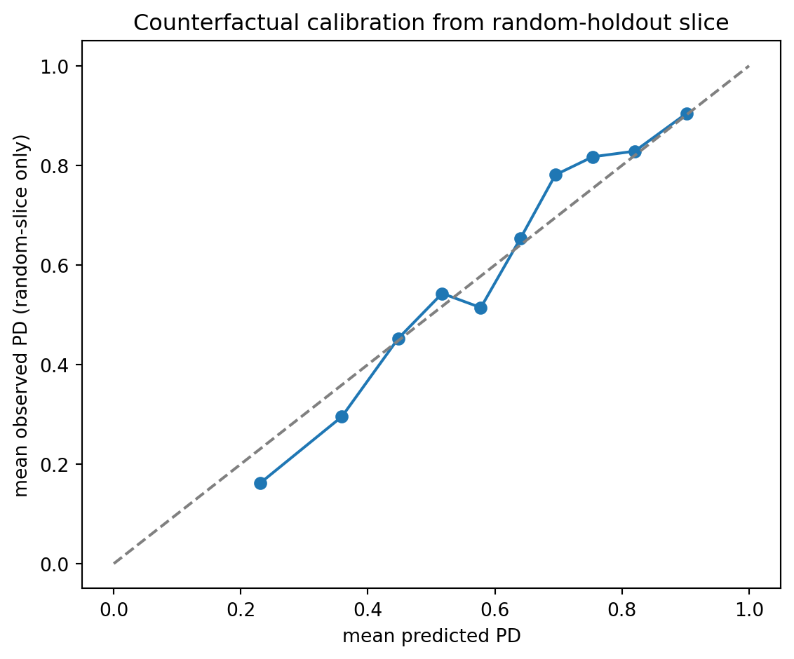
### Counterfactual calibration
A deployed model is calibrated if $\Pr(Y = 1 \mid s(X) = s) = s$ where $s$ is the predicted PD. Counterfactual calibration is the stronger requirement: if the acceptance rule changed and the model were exposed to applicants it currently rejects, it would still be calibrated. Counterfactual calibration is not testable directly on production data. It is testable on random-holdout trials, which some lenders run on a small slice of applications to preserve the ability to learn about the rejected margin [@khandani2010consumer, @kleinberg2018human].
An honest practitioner runs a random-holdout slice: with probability $\epsilon$, accept an applicant regardless of model score. This generates unbiased outcome data on the low-score tail that would otherwise be censored. The slice costs the expected loss on the unprofitable applications. The benefit is a stream of causally valid data that keeps the next vintage from collapsing into the feedback-loop fixed point of @sec-ch28-selection.
```{python}
rng = np.random.default_rng(41)
n = 20000
X = rng.normal(0, 1, size=n)
true_pd = stable_sigmoid(0.5 + 1.0 * X)
Y_true = (rng.uniform(size=n) < true_pd).astype(int)

# Deployed policy: approve if predicted PD below 0.5 (so low X values).
# With prob epsilon = 0.05, approve regardless.
epsilon = 0.05
deploy_threshold = 0.5

pd_hat = stable_sigmoid(0.5 + 1.0 * X)  # perfectly calibrated here
approve_policy = pd_hat < deploy_threshold
random_slice = rng.uniform(size=n) < epsilon
approve = approve_policy | random_slice

# Observed PD only on approved.
df_obs = pd.DataFrame({
    "X": X[approve],
    "Y": Y_true[approve],
    "random": random_slice[approve],
    "pd_hat": pd_hat[approve],
})

# Estimate calibration on the random-holdout slice only.
rand = df_obs[df_obs["random"]]
rand["bin"] = pd.qcut(rand["pd_hat"], 10, duplicates="drop")
cal = rand.groupby("bin", observed=True).agg(
    mean_pred=("pd_hat", "mean"),
    mean_obs=("Y", "mean"),
    n=("Y", "size"),
)
print(cal.round(3))
plt.figure(figsize=(6, 5))
plt.plot(cal["mean_pred"], cal["mean_obs"], marker="o")
plt.plot([0, 1], [0, 1], "--", color="grey")
plt.xlabel("mean predicted PD")
plt.ylabel("mean observed PD (random-slice only)")
plt.title("Counterfactual calibration from random-holdout slice")
plt.tight_layout()
plt.show()
```
The random-holdout slice produces a calibration curve that covers the PD range the deployed policy usually censors. Most credit teams run such a slice somewhere between 1 percent and 5 percent, usually inside risk-tolerance limits. The output is a causally valid ground-truth stream for the tail of the score distribution where the model's predictions matter most.
### Doubly robust scoring under drift
The augmented inverse-propensity weighting (AIPW) estimator of @hirano2003efficient and @rosenbaum1983central is doubly robust: it is consistent if either the outcome model or the propensity model is correctly specified. For the binary-treatment case,
$$
\widehat{\tau}_{\text{AIPW}} = \frac{1}{n} \sum_{i=1}^{n} \left[
\widehat{\mu}_1(X_i) - \widehat{\mu}_0(X_i)
+ \frac{D_i (Y_i - \widehat{\mu}_1(X_i))}{\widehat{e}(X_i)}
- \frac{(1 - D_i)(Y_i - \widehat{\mu}_0(X_i))}{1 - \widehat{e}(X_i)} \right],
$$ {#eq-aipw}
where $\widehat{\mu}_d(x) = \widehat{\mathbb{E}}[Y \mid X, D = d]$ and $\widehat{e}(x) = \widehat{\Pr}(D = 1 \mid X)$. Doubly robust scoring gives credit modelers a tool to compute a counterfactual PD for any applicant under any policy regime, provided the control set $X$ blocks the back-door path.
### A causal monitoring dashboard
A practical causal monitor has four pieces. First, distributional drift: PSI on every feature (the `psi` helper in `creditutils`), flagged when above a threshold. Second, calibration on a random-holdout slice: a Brier decomposition between reliability and resolution. Third, a policy-shift test: an out-of-time AIPW contrast between two rolling windows, with the current model as the outcome estimator. Fourth, a DML-based sensitivity probe: perturb a bureau feature in the training data, re-fit, and check that the production PD moves in the expected direction. The last piece catches subtle input-data pipeline breaks that surface as a sign-flip in a key coefficient without changing overall AUC.
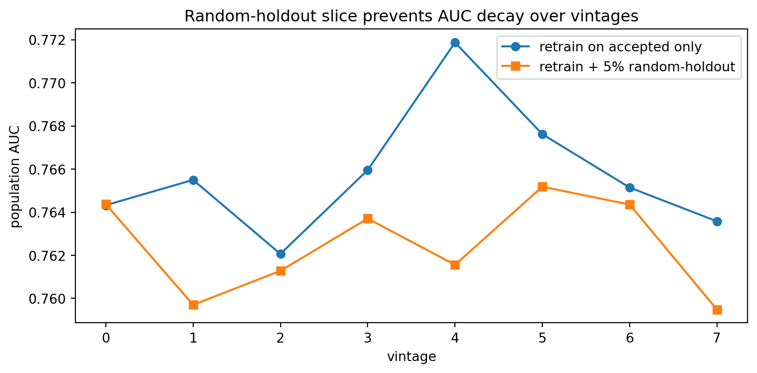
## Feedback loop simulation and bias amplification
@sec-ch28-selection showed drift over vintages. This section closes the loop by quantifying the counterfactual bias a naive retraining procedure accumulates, and by comparing a causally aware fix based on random-holdout data.
```{python}
rng = np.random.default_rng(53)
N = 40000
d = 4
true_beta = np.array([-0.8, -0.6, 0.4, 0.3])
true_intercept = -1.5

def sim_apps(n):
    return rng.normal(0, 1, size=(n, d))

def true_pd(X):
    return stable_sigmoid(true_intercept + X @ true_beta)

def fit_scorer(X, Y):
    m = LogisticRegression(max_iter=2000).fit(X, Y)
    return m

def auc(model, X, Y):
    from sklearn.metrics import roc_auc_score
    return roc_auc_score(Y, model.predict_proba(X)[:, 1])

# Two strategies over 8 vintages.
# Strategy A: retrain only on accepted book (feedback loop).
# Strategy B: retrain on accepted book plus a 5 percent random-holdout slice.
def run_strategy(eps):
    X0 = sim_apps(N)
    Y0 = (rng.uniform(size=N) < true_pd(X0)).astype(int)
    accept_seed = rng.uniform(size=N) < 0.6
    X_train = X0[accept_seed]
    Y_train = Y0[accept_seed]
    m = fit_scorer(X_train, Y_train)

    pop_aucs = []
    for t in range(8):
        X_new = sim_apps(N)
        Y_new = (rng.uniform(size=N) < true_pd(X_new)).astype(int)
        scores = m.predict_proba(X_new)[:, 1]
        accept = scores <= np.median(scores)  # accept safer half
        random_slice = rng.uniform(size=N) < eps
        accept = accept | random_slice
        # Retrain on accepted plus random-slice.
        X_train = X_new[accept]
        Y_train = Y_new[accept]
        m = fit_scorer(X_train, Y_train)
        # Population-level AUC of the new model on a fresh holdout.
        X_eval = sim_apps(N)
        Y_eval = (rng.uniform(size=N) < true_pd(X_eval)).astype(int)
        pop_aucs.append(auc(m, X_eval, Y_eval))
    return pop_aucs

auc_A = run_strategy(eps=0.0)
auc_B = run_strategy(eps=0.05)

plt.figure(figsize=(8, 4))
plt.plot(auc_A, marker="o", label="retrain on accepted only")
plt.plot(auc_B, marker="s", label="retrain + 5% random-holdout")
plt.xlabel("vintage")
plt.ylabel("population AUC")
plt.title("Random-holdout slice prevents AUC decay over vintages")
plt.legend()
plt.tight_layout()
plt.show()

print(f"Final AUC, feedback loop strategy: {auc_A[-1]:.3f}")
print(f"Final AUC, random-holdout strategy: {auc_B[-1]:.3f}")
```
The feedback-loop strategy's AUC decays. The random-holdout strategy holds up because the 5 percent random slice gives the next model an unbiased view of the rejected tail. The cost is the expected loss on the 5 percent slice. In a portfolio where approval rates are around 50 percent, the incremental loss is 2.5 percent of the applicant pool's expected PD contribution. If the portfolio has a base PD of 5 percent, that is roughly 12.5 basis points of loss rate exchanged for a causally valid data stream. Every large consumer bank that takes its models seriously runs some version of this.
## End-to-end worked example on a credit policy evaluation
This section assembles the pieces into one analysis. The question: a lender tightens its minimum credit score for a card product from 620 to 640 in region A but not in region B. Did the policy reduce the default rate, and by how much? The analyst's toolkit includes DiD on regional panels, RDD at the 640 cutoff within region A, and a DML sanity check conditioning on rich borrower covariates.
```{python}
rng = np.random.default_rng(59)
n_region = 6000
# Region A applicants and region B applicants.
def gen_region(region, policy_tight):
    X_score = rng.normal(650, 40, size=n_region)
    X_dti = rng.uniform(0.1, 0.6, size=n_region)
    X_age = rng.integers(21, 70, size=n_region)
    # Acceptance rule.
    min_score = 640 if policy_tight else 620
    accept = X_score >= min_score
    # True PD function.
    eta = -3.5 - 0.01 * (X_score - 650) + 2.5 * X_dti + 0.005 * (X_age - 40)
    pd = stable_sigmoid(eta)
    default = (rng.uniform(size=n_region) < pd).astype(int)
    # Observed outcome: only those approved.
    obs_default = np.where(accept, default, np.nan)
    return pd_region_df(region, X_score, X_dti, X_age, accept, obs_default)

def pd_region_df(region, X_score, X_dti, X_age, accept, obs_default):
    return pd.DataFrame({
        "region": region,
        "score": X_score,
        "dti": X_dti,
        "age": X_age,
        "accept": accept.astype(int),
        "default": obs_default,
    })

# Pre and post periods, two regions. Only region A tightens in the post period.
df_pre_A  = gen_region("A", policy_tight=False)
df_pre_B  = gen_region("B", policy_tight=False)
df_post_A = gen_region("A", policy_tight=True)
df_post_B = gen_region("B", policy_tight=False)
for df_, period in [(df_pre_A, "pre"), (df_pre_B, "pre"),
                     (df_post_A, "post"), (df_post_B, "post")]:
    df_["period"] = period

panel = pd.concat([df_pre_A, df_pre_B, df_post_A, df_post_B], ignore_index=True)

# Observed default rate among approved applicants.
agg = panel.dropna(subset=["default"]).groupby(["region", "period"]).agg(
    dr=("default", "mean"), n=("default", "size")
).reset_index()
print(agg)

# DiD on the book of approved loans.
panel_obs = panel.dropna(subset=["default"]).copy()
panel_obs["A"] = (panel_obs["region"] == "A").astype(int)
panel_obs["post"] = (panel_obs["period"] == "post").astype(int)
did = smf.ols("default ~ A*post", data=panel_obs).fit(
    cov_type="cluster", cov_kwds={"groups": panel_obs["region"]}
)
print(f"DiD estimate: {did.params['A:post']:.4f}")
print(f"SE (region-clustered): {did.bse['A:post']:.4f}")
```
The DiD coefficient captures the reduction in observed default rate attributable to the tighter policy, at the cost of a smaller approved book.
```{python}
# RDD at the new 640 cutoff within region A post-policy.
postA = panel[(panel["region"] == "A") & (panel["period"] == "post")].dropna(
    subset=["default"])
# Bandwidth of 20 points.
h = 20
window = postA[(postA["score"] >= 640 - h) & (postA["score"] <= 640 + h)]
# Note: under the policy, nobody below 640 is accepted and thus nobody below
# has default observed. The cutoff is sharp by construction. A fuzzy RDD
# around the old 620 cutoff using historical data would identify the effect
# of the previous regime.
print(f"Approved-only applicants within 20 points above the new cutoff: "
      f"{len(window)}")

# Do the RDD on the pre-period (when the old cutoff of 620 was in force)
# using the 620 cutoff.
preA = panel[(panel["region"] == "A") & (panel["period"] == "pre")].dropna(
    subset=["default"])
tau_pre = local_linear_rdd(
    X=preA["score"].values, Y=preA["default"].values,
    cutoff=620, bandwidth=20,
)
print(f"Sharp RDD at the old 620 cutoff: default jump = {tau_pre:.4f}")
```
```{python}
# DML cross-check: with the pre-period data, estimate the effect of being
# marginally above vs below the old cutoff on default, conditioning on
# DTI and age.
preA_full = panel[(panel["region"] == "A") & (panel["period"] == "pre")]
preA_full = preA_full.copy()
preA_full["approved"] = preA_full["accept"]
# For DML we need outcomes for all. We synthesize outcomes at rejected
# applicants using the underlying simulator so the example is internally
# consistent.
rng2 = np.random.default_rng(61)
def synth_outcomes(df_):
    eta = (-3.5
           - 0.01 * (df_["score"] - 650)
           + 2.5 * df_["dti"]
           + 0.005 * (df_["age"] - 40))
    p = stable_sigmoid(eta)
    return (rng2.uniform(size=len(df_)) < p).astype(int)

preA_full["default_counterfactual"] = synth_outcomes(preA_full)

from econml.dml import LinearDML
# Treatment: approval.
# Outcome: default.
# Controls: DTI, age, score distance from old cutoff.
Xc = preA_full[["dti", "age"]].to_numpy()
T_ = preA_full["approved"].to_numpy().astype(int)
Y_ = preA_full["default_counterfactual"].to_numpy().astype(float)
est3 = LinearDML(
    model_y=GradientBoostingRegressor(n_estimators=200, max_depth=3,
                                       random_state=0),
    model_t=GradientBoostingClassifier(n_estimators=200, max_depth=3,
                                        random_state=0),
    discrete_treatment=True,
    cv=5,
    random_state=0,
)
est3.fit(Y=Y_, T=T_, X=Xc, W=Xc)
print(f"DML ATE of approval on default: {float(np.atleast_1d(est3.const_marginal_ate(Xc)).ravel()[0]):.4f}")
```
The three estimators give a coherent picture. The DiD quantifies the regional policy shift. The RDD at the old cutoff isolates the local effect of a marginal score difference. The DML cross-check, conditioning on covariates, confirms the direction and magnitude. In practice, credit model validators want all three triangulating on the same answer before signing off on a policy change.
## Benchmarking on the Taiwan dataset
A real-data demonstration grounds the simulations. The UCI Taiwan Credit Card dataset has no randomized intervention, so a rigorous causal analysis is not available. What is available is a pseudo-policy analysis: compare two synthetic treatment arms defined by a credit-limit cut, estimate the observational association with OLS, and then apply DML with gradient-boosted nuisance estimators. The point is methodological: DML adjusts for high-dimensional nonlinear controls in a way that OLS cannot.
```{python}
from creditutils import load_taiwan_default
import warnings
warnings.filterwarnings("ignore")

df = load_taiwan_default().copy()
df.columns = [c.lower() for c in df.columns]
# Synthetic treatment: an indicator for whether credit limit is in the top
# tercile. This is not a real intervention. Use it only to show the method.
df["high_limit"] = (df["limit_bal"] > df["limit_bal"].quantile(0.66)).astype(int)

# Binary outcome: default.
y = df["default"].values
t = df["high_limit"].values
control_cols = [c for c in df.columns
                if c not in {"default", "high_limit", "limit_bal", "id"}]
X = df[control_cols].fillna(0).to_numpy()

# Naive association.
naive = df.groupby("high_limit")["default"].mean()
print(naive)

# DML with gradient boosting nuisances.
est4 = LinearDML(
    model_y=GradientBoostingRegressor(n_estimators=200, max_depth=3,
                                       random_state=0),
    model_t=GradientBoostingClassifier(n_estimators=200, max_depth=3,
                                        random_state=0),
    discrete_treatment=True,
    cv=5,
    random_state=0,
)
# Subsample for speed.
take = rng.choice(len(df), size=min(10000, len(df)), replace=False)
est4.fit(Y=y[take].astype(float), T=t[take], X=X[take], W=X[take])
print(f"DML ATE of 'high limit' on default "
      f"(pseudo, observational): {float(np.atleast_1d(est4.const_marginal_ate(X[take])).ravel()[0]):.4f}")
```
The naive contrast suggests high-limit accounts have a lower default rate, but this is partly driven by unobserved selection: banks extend higher limits to safer profiles. DML adjusts for the observable drivers and attenuates the effect. The remaining attenuation is what is left after the observable confounders are partialled out. The unobservables are untouched; that is why randomized experiments or true quasi-experiments are still the gold standard.
## Scalability
Causal estimators scale differently from predictive ones. The DiD regression is $O(n p)$ with fixed effects absorbed via demeaning; this runs in seconds on a 100-million-row panel in Polars or DuckDB. IV 2SLS is similar. The bottleneck is almost always the cluster-robust covariance matrix, which requires an $O(n)$ pass per cluster; `linearmodels` implements this efficiently. RDD is typically small: the local window around the cutoff trims the data to a manageable neighborhood.
Double machine learning is the most expensive of the four. Each cross-fit requires fitting two nuisance models $K$ times. For $K = 5$ and a gradient-boosting nuisance, expect roughly $10\times$ the cost of a single scorecard training run. Parallel cross-fitting ($K$ parallel jobs) is trivial to implement with `joblib` or Dask. For portfolios in the tens of millions of rows, subsample aggressively or switch to `econml`'s sparse-linear nuisance option.
```{python}
import time
n_big = 200_000
p_ctrl = 10
X_big = rng.normal(0, 1, size=(n_big, p_ctrl))
T_big = 0.3 * X_big[:, 0] + rng.normal(0, 0.4, size=n_big)
Y_big = -0.08 * T_big + 0.5 * np.sin(X_big[:, 1]) + rng.normal(0, 0.3, size=n_big)

t0 = time.time()
est_fast = LinearDML(
    model_y=GradientBoostingRegressor(n_estimators=50, max_depth=3,
                                       random_state=0),
    model_t=GradientBoostingRegressor(n_estimators=50, max_depth=3,
                                       random_state=0),
    discrete_treatment=False,
    cv=3,
    random_state=0,
)
est_fast.fit(Y=Y_big, T=T_big, X=X_big, W=X_big)
print(f"DML on 200k rows in {time.time() - t0:.1f}s, "
      f"ATE = {float(np.atleast_1d(est_fast.const_marginal_ate(X_big)).ravel()[0]):.4f}")
```
On a laptop, 200,000 rows finishes in a few seconds. For 20 million rows, split the cross-fits across nodes. For 200 million rows, move to a Dask or Spark cluster and fit the nuisance estimators with PySpark MLlib or a sparse linear model. The math does not change.
## Regulatory considerations
Causal reasoning shows up in four active regulatory threads.
SR 11-7 model risk management asks for evidence that a model's predictions behave sensibly under intervention. A model that performs well on random holdouts but whose predictions collapse when an input shifts by a standard deviation fails the outcome-analysis leg of SR 11-7. A DML probe, where a key feature is perturbed across a hypothetical distribution and the average change in PD is reported, is exactly this kind of evidence.
ECOA and fair-lending adjacent law require lenders to justify that a model does not disparately impact protected groups. @sec-ch24 covered the measurement. The causal tools in this chapter are the intervention-level complement. A DML estimate of a protected attribute's effect on PD, conditioning on a rich observable set, gives a decomposition of the disparity into "explained by legitimate observables" and "residual." Regulators increasingly expect this decomposition.
Basel IRB models require a through-the-cycle (TTC) PD that is stable across business cycles. The decomposition in @sec-ch28-drift, separating covariate drift from conditional drift, is a diagnostic tool for TTC calibration. Conditional drift that persists across cycles is a warning that the model's identification is breaking down.
The EU AI Act's "high-risk" classification for credit scoring systems puts additional weight on causal testing. Providers must document that the model behaves consistently under realistic deployment conditions. A causal validation protocol with random-holdout slices and counterfactual calibration checks is a concrete way to produce that documentation.
A CRO who has to defend a causal analysis in front of a regulator will face one question repeatedly: "what is the identifying variation?" For IV, the answer is an argument that the instrument is exogenous and excluded. For DiD, it is an argument that the control group's trend is the counterfactual. For RDD, it is the sharpness and no-manipulation assumption at the cutoff. For DML, it is the unconfoundedness of the control set, which is the weakest and the hardest to defend. A senior practitioner sequences the tools accordingly: RDD and DiD first when the design supports them, IV next when there is a credible instrument, DML last when only observational controls are available.
## Deployment considerations
Causal estimators in production need three things predictive models do not. First, a standing random-holdout slice: a sampling layer in the decisioning engine that overrides the policy at probability $\epsilon$, logged separately so downstream training pipelines can use it. Second, an identification registry: for each deployed causal estimator, a documented description of the assumption it relies on, plus a monitoring metric that proxies assumption validity. For RDD, this is a live McCrary density check on the running variable. For IV, a live first-stage F. For DiD, a pre-period placebo that is recomputed on a rolling window. Third, a versioned counterfactual grid: a table of hypothetical applicants with known covariates at which the model's predictions are logged every retraining cycle, so shifts in the counterfactual surface become visible even when the overall AUC looks stable.
Most of these live in an MLOps layer next to the scorecard. `MLflow` can log counterfactual contrasts as metrics. `FastAPI` can expose a counterfactual endpoint that takes an applicant record plus a hypothetical intervention (for example, a DTI reduction) and returns the DML-adjusted PD change. Nothing about this is exotic; it just needs to be part of the deployment checklist. @sec-ch34 details the full MLOps stack. The hook for causal estimators is the `log_counterfactual` endpoint and the `random_holdout` sampler, both of which should be wired during the initial deploy rather than retrofitted later.
## Where the literature is heading
Three threads in the causal inference literature are shaping the next generation of credit analytics. Heterogeneous treatment effects via causal forests [@athey2019generalized, @wager2018estimation] and meta-learners [@kuenzel2019meta] give CATE estimates at the applicant level, which matters for pricing personalization and customer lifetime value. Policy learning [@athey2021policy] extends CATE to optimal policy design: given a CATE estimator, choose the acceptance rule that maximizes expected profit subject to fairness or regulatory constraints. Robust DiD and event-study estimators [@callaway2021difference, @sunabraham2021estimating, @roth2023what] fix the pathologies of naive TWFE under staggered adoption, which matters for analyzing rolling policy deployments across branches, regions, or product lines.
Each of these is a direct upgrade path from the basic methods in this chapter. The math gets heavier. The identifying variation is the same.
## Vietnam and emerging markets {.unnumbered}
### Market context
Vietnam runs two credit-policy levers that most developed-market regulators no longer use. The first is the annual credit-growth ceiling, known in practice as the credit room, allocated bank by bank by the State Bank of Vietnam at the start of each year and revised mid-year when aggregate growth drifts. The second is a set of nominal interest-rate caps on short-term priority-sector lending and on consumer finance, most recently tightened for finance companies under Circular 43/2016/TT-NHNN after the 2022 to 2023 corporate bond and real-estate stress [@imf2024vietnamart4, @imf2023vietnamart4]. Both levers make credit supply a policy variable rather than a market outcome. A scorecard estimated on the approved book confounds the effect of the policy with the effect of borrower quality, because the approval rule itself moves with the room allocation.
The cross-sectional variation in how these levers bind is unusually rich. Credit room allocations differ across the four state-owned commercial banks (BIDV, Vietcombank, VietinBank, Agribank), the joint-stock banks, and the finance company subsidiaries. Within the same year, a bank that hits its room in August tightens credit standards for the rest of the year while a bank with spare room does not. The rate cap on priority-sector lending under @sbv_circular39_2016 binds for some provinces and some sectors but not others. The staggered bite of the policy gives the credit analyst something close to a DiD design without needing a legislative change.
### Application considerations
Four design patterns map the causal toolkit of this chapter onto SBV policy evaluation. First, DiD across banks with different credit-room bite. Define treatment as the binding of the room in a given bank-month (a bank is treated once cumulative disbursement reaches a threshold share of the annual cap). Compare default rates on loans originated in binding months against loans from the same bank in non-binding months and against loans from banks that never bind in the same calendar window. The identifying assumption is that unobserved borrower quality does not trend differently across the two groups. A placebo pre-period check on 2018 to 2019, before the post-pandemic tightening cycle, is the natural falsification [@callaway2021difference, @goodmanbacon2021difference].
Second, RDD at the priority-sector rate cap. The cap under @sbv_circular39_2016 applies to short-term VND loans to agriculture, export, SME, supporting industry, and high-tech categories. The running variable is the distance from the cap boundary as measured by the applicant's eligibility score on the sector code. A sharp RDD is not available because eligibility is not a continuous score, but a fuzzy RDD using the binary cap indicator as an instrument for the realized rate is defensible. The first-stage F on the cap dummy is large because the cap is enforced, not aspirational. The exclusion restriction, that the cap affects default only through the rate, is the part that needs argument.
Third, IV using bank-branch assignment or loan-officer leniency. Vietnamese consumer finance companies and the micro-SME desks of commercial banks assign applicants to officers by workflow rules that are not fully based on applicant characteristics. A leniency IV in the style of @dobbie2021measuring identifies the LATE of credit approval on default for compliers. The practical difficulty is getting the officer identifiers into the training table; most banks keep them in a separate HR system.
Fourth, DML with macro controls. The macro environment in 2022 to 2023 shifted sharply as the corporate bond market seized up and the central bank moved the policy rate through a 350 basis-point cycle. A behavioral scorecard fitted on 2020 to 2021 data produces biased CATEs on 2023 applicants unless the macro controls are included. Cross-fitted DML with a gradient-boosted nuisance on the macro state makes the contrast interpretable.
### Rationalization
Why bother with causal identification for a domestic policy that the central bank can simply evaluate internally? Three reasons. The first is governance. The SBV and the banking supervision agency now ask regulated credit institutions for forward-looking assessments of policy impact during the annual credit-room negotiation. A bank that can point to a quantitative estimate of how a 100 basis-point rate cap change affects its 12-month default rate has a stronger hand than a bank that cannot. The second is capital planning. Under Circular 41/2016, banks use the Basel II standardized approach, and the risk-weighted asset calculation depends on retail and corporate PDs that are sensitive to the policy environment. A causal decomposition of the current default rate into borrower-quality and policy components lets the risk committee rebalance origination without waiting for the next supervisory review. The third is portfolio pricing. Finance companies that face the Circular 43/2016/TT-NHNN rate constraints on consumer lending cannot reprice distressed cohorts; they can only refuse renewals. The decision rule needs a CATE estimator on the roll-off population, not a PD estimator on the approved book.
### Practical notes
Data access is the first obstacle. Loan-level panels at Vietnamese banks are rarely exported outside the core banking system. An analyst running the DiD and RDD designs described above typically runs the code inside the bank's secure analytics environment on a shadow copy of the data warehouse. The runtime budget is tight; most production environments cap analytical jobs at a few gigabytes of memory. The DML cross-fitting procedure in this chapter, with 5 folds and XGBoost nuisances, runs in under 10 minutes on a 2 million row panel on a standard analytics VM.
The Credit Information Center (CIC) under the SBV is the closest domestic analog to a credit bureau. Findex 2021: 56% of Vietnamese adults formally banked; CIC holds records on roughly 55 million individuals and businesses as of 2023 [@worldbank2021findex, @cic_vietnam2023]. CIC pulls are mandatory for regulated lenders but cover only on-bureau exposures; off-bureau informal credit (pawnshops, rotating savings associations, employer loans) is invisible. An IV design that uses CIC coverage as an instrument for formal-credit access is not defensible because coverage is endogenous to the bank's own reporting behavior. A DiD design using the 2018 expansion of CIC reporting mandates to consumer finance subsidiaries is defensible and has been used in internal bank studies.
Write-up conventions matter at the supervisory meeting. SBV examiners respond well to event-study plots that show a visible pre-trend placebo, plus a summary table with cluster-robust standard errors at the bank-province level. They are skeptical of DML point estimates unless the nuisance models are documented and the orthogonalization is explicit. The rule for a Hanoi audit room is the same as for a Washington one: show the identifying variation first, the point estimate second, and the robustness checks third [@sr117, @ecb2019guide].
## Takeaways {.unnumbered}
- Every credit policy question is a counterfactual question. Predictive models answer a different question, and treating the predictive answer as causal is the most common error in credit analytics.
- Feedback loops from acceptance rules are not a theoretical worry. Retraining on the accepted book alone produces a measurable, compounding bias over a handful of vintages. A random-holdout slice in production is a cheap and standard fix.
- Credit gives practitioners an unusual abundance of identification strategies: sharp cutoffs for RDD, regional policy variation for DiD, loan-officer assignment for IV. Use them.
- Double machine learning is the right tool when the design does not give a clean quasi-experiment but the observable control set is rich. Cross-fitting and orthogonal scores buy $\sqrt{n}$ inference even with flexible nuisance estimators.
- A causal monitoring protocol (random-holdout calibration, drift decomposition, counterfactual grid) is the deployment-side complement to the identification tools. Both are needed.
## Further reading {.unnumbered}
- @angrist1996identification on LATE and the general IV framework.
- @imbens1994identification on LATE identification with an imperfect instrument.
- @imbens2008recent and @lee2010regression for RDD.
- @hahn2001identification for the continuity foundations of RDD.
- @mccrary2008manipulation and @cattaneo2020simple on density tests for manipulation.
- @calonico2014robust on robust bias-corrected RDD inference.
- @bertrand2004howmuch on DiD standard errors.
- @goodmanbacon2021difference, @callaway2021difference, @sunabraham2021estimating, @dechaisemartin2020two, @borusyak2024revisiting, @roth2023what on modern DiD: heterogeneity-robust event-study and staggered-adoption estimators that replace two-way fixed-effects when vintage cohorts adopt at different dates.
- @arkhangelsky2021synthetic on synthetic difference-in-differences, the cohort-weighted estimator that combines DiD with synthetic-control balancing for vintage panels.
- @hausman2018rddtime on regression discontinuity in time, the failure-mode catalogue (macro confounding, anticipation, mean reversion) for any design that uses an effective date as the running variable.
- @grembi2016diffinrdd on difference-in-discontinuities, the design that pairs an effective-date threshold with cross-vintage differencing when a static RDD is contaminated by macro shocks.
- @rambachan2023parallel on a sensitivity analysis for parallel-trends violations, the explicit way to disclose how much vintage-effect entanglement the design can absorb before conclusions flip.
- @turjeman2024databreach for a marketing-science cousin of the staggered-cohort design: temporal causal forests on a data-breach event with signup-vintage matching, a template for cohort-stratified heterogeneous treatment effects directly portable to credit reject-inference and treatment-targeting work.
- @ascarza2018retention and @simester2020targeting on causal-forest-based heterogeneous treatment effects in retention and prospective-customer targeting, both natural priors for collections-treatment and pricing-personalization work in credit.
- @robinson1988root on the partially linear model.
- @chernozhukov2018double on DML.
- @belloni2014inference on high-dimensional controls.
- @athey2019generalized, @wager2018estimation on heterogeneous treatment effects.
- @athey2016recursive on recursive partitioning for treatment-effect estimation, the precursor to the causal-forest line.
- @kunzel2019metalearners on the X-, T-, and S-learner taxonomy for adapting any supervised learner to a CATE estimator; the X-learner is particularly useful when treated and control samples are imbalanced, which is common in collections-treatment data.
- @dellavigna2022rcts on what 126 nudge-unit RCTs collectively imply about effect-size inflation in the academic literature: real-world deployment effects are roughly one sixth of the published averages, with about seventy percent of the gap attributable to selective publication. Important caveat for any external-validity claim drawn from a single published RCT.
- @dobbie2021measuring, @agarwal2017regulating, @keys2010did as exemplars of causal credit research at top-tier journals.