---
bibliography:
- ../references.bib
- ../refs/ch-01.bib
execute:
echo: true
eval: true
warning: false
---
# Introduction and Historical Development {#sec-ch01}
::: {.callout-note appearance="simple" icon="false"}
**Scope: both retail and corporate.** Surveys consumer scoring (FICO, scorecards) and corporate distress modeling (Altman Z, Ohlson O, Merton) as one historical lineage.
:::
## Why a book on credit scoring {.unnumbered}
A credit score is a conditional expectation. Given what a lender can observe about a borrower at the moment of decision, a score is an estimate of the probability that the borrower will fail to meet a contractual obligation over some horizon. Every decision that follows, whether to extend credit, at what price, against what collateral, with what limit, is a function of that estimate and its uncertainty. This book is about how to construct that estimate well.
The problem has three features that, together, make credit scoring distinct from generic binary classification. First, the ground truth is expensive and delayed. A default observation arrives months or years after the decision, and often only for the subset of applicants the lender chose to accept, so the training distribution is selected. Second, decisions are regulated. The Equal Credit Opportunity Act, the Fair Credit Reporting Act, Basel III, IFRS 9, CECL, SR 11-7, GDPR Article 22, and the EU AI Act all impose hard constraints on what features can be used, how models must be documented, how risk-weighted assets are computed, and how losses are provisioned. Third, the consumer side is large, roughly 18 trillion US dollars of household debt in the United States as of 2024 according to the Federal Reserve, with billions of dollars in interest and fees flowing through scoring systems every day. Small improvements in discrimination compound into large profit-and-loss effects and large welfare effects.
The goals of this book are narrow and concrete. For the practitioner, we derive every method from scratch, implement it in NumPy or PyTorch, and then call the same standard library that a risk team would run in production. For the academic, we cite the primary literature in top-tier venues and benchmark each method on the same three public datasets so that results are comparable across chapters. For the regulator or supervisor, we tie every technique to the supervisory text that constrains its use. We prefer working code over narrative, and working math over intuition.
This first chapter is the only one without a single estimator as its core object. Its job is to explain why the field exists, how it arrived at its current shape, and how the rest of the book is organized. A short empirical section fits a logistic scorecard on the two canonical public datasets. That baseline recurs throughout later chapters as a reference point for every more elaborate method.
A word to the practitioner in an emerging market. The institutional history in this chapter is Anglo-American because the primary sources and the regulatory templates are. The modeling problems are not. A Vietnamese consumer-finance lender, an Indonesian digital bank, a Kenyan mobile-money scorer, and a Brazilian fintech share a set of features that mid-1990s US scorecard literature did not contemplate: thin-file or no-file borrowers, a cash economy with self-reported income, a credit bureau whose coverage is partial and whose tradeline depth is shallow, and a distribution channel that is mobile-first from the first customer touch. Every chapter from here on has to be read twice: once for the US or EU template, once for what needs to be re-derived, rebalanced, or replaced when the bureau carries half the adult population and half the income is informal.
## Why credit scoring exists {#sec-ch01-intro}
### Information asymmetry as the core friction
The theoretical justification for credit scoring was provided in two papers written eleven years apart. The first is @akerlof1970lemons. Akerlof showed that when sellers know more about product quality than buyers, the market can unravel. Low-quality goods crowd out high-quality goods because buyers, unable to distinguish, price-average. Owners of high-quality goods withdraw, the average quality drops, prices drop further, and the market collapses toward the lowest quality or disappears altogether. The argument is a one-paragraph proof of the welfare cost of asymmetric information.
The second is @stiglitz1981credit. Stiglitz and Weiss adapted Akerlof's logic to credit markets. A bank cannot perfectly observe the riskiness of a loan applicant. If it raises the interest rate to compensate for unobserved risk, it worsens the pool of applicants, because safe borrowers have lower reservation rates and drop out, while risky borrowers, whose upside is bounded by success and whose downside is bounded by default, remain. The result is credit rationing: in equilibrium, banks prefer to cap quantity rather than clear the market with price, and some creditworthy borrowers are rejected. This is the adverse-selection side of the story.
There is also a moral-hazard side. Once a loan is made, the borrower can take unobservable actions, whether to invest the proceeds productively, to maintain insurance, to honor the repayment plan when default is unattractive but legal, that affect repayment. Under moral hazard, contracts and monitoring become the margins of adjustment [@holmstrom1979moral; @townsend1979optimal]. Screening at origination addresses selection; monitoring during the life of the loan addresses moral hazard. A credit score is primarily a screening device, although behavioral scores used after origination are monitoring devices.
Earlier work laid the foundation. @spence1973job showed how informed parties can signal quality through costly actions. @rothschild1976equilibrium analyzed how uninformed insurers can screen by offering menus of contracts. @jaffee1976imperfect argued credit rationing arises when loan supply functions become backward-bending under default risk. @diamond1984financial showed that a delegated monitor, the bank, can resolve the free-rider problem among dispersed creditors by aggregating monitoring costs. @diamond1991monitoring sharpened the argument into a theory of the choice between bank loans and public debt, with reputation and screening as the relevant margins.
A simple numerical illustration makes the Stiglitz-Weiss mechanism concrete. Suppose borrowers come in two unobservable types, safe and risky, each drawn with equal probability. Safe projects pay back a fixed amount $R_s$ with certainty. Risky projects pay back a larger amount $R_r > R_s$ with probability $p$ and zero with probability $1 - p$. A bank that sets interest rate $r$ faces the participation margin: safe borrowers accept only if $R_s \ge 1 + r$, while risky borrowers accept if $p \cdot R_r \ge p \cdot (1 + r)$, that is, whenever $R_r \ge 1 + r$. Because $R_r > R_s$, any rate high enough to drive safe borrowers out still attracts risky ones. The expected return to the bank is non-monotone in $r$: raising $r$ increases revenue per contract but worsens the mix. At some $r^*$ the two effects exactly cancel; above it, expected profit falls. The bank's optimal policy caps $r$ at $r^*$ and rations quantity at that rate. The welfare loss is the mass of safe borrowers who would have borrowed at rates just above $R_s - 1$, and the bank would have lent to them, except that the rate required to break even on the pooled portfolio is unacceptable to the safe type. Credit scoring resolves the friction by conditioning the offer on an observable signal that is correlated with type.
The costly-state-verification argument of @townsend1979optimal takes a different route to the same destination. In Townsend's setup, the borrower knows her return but the lender can verify it only by paying a verification cost. The optimal contract is a standard debt contract: the borrower pays a fixed amount in non-default states, and the lender verifies only in default. The verification cost is the economic rent the lender extracts, and scoring reduces that rent by lowering the probability of default ex ante. @holmstrom1979moral's moral-hazard setup generates a different implication: when effort is unobservable, the first-best is not implementable and the contract must make the borrower's payment contingent on the outcome. Scoring affects this setup through the participation constraint, not the incentive constraint, because it improves the ex-ante distribution of the contract partners.
The screening-versus-relationship view connects back to banking structure. @hauswald2006information model how a bank's informational advantage from screening is eroded by competitor acquisition of the same signals, which changes the equilibrium compensation for screening effort. @liberti2019information formalize the distinction between hard information (codifiable, transferable across the org) and soft information (subjective, context-dependent, tied to the loan officer) and show how the two interact as scoring technology improves. For the practitioner, the takeaway is that the value of a scoring system is not just the loss reduction it delivers on accepted loans. It is the change in the whole portfolio allocation induced by conditioning on a predictive signal.
### Screening versus monitoring
A useful distinction for the rest of this book is between screening (ex ante, before credit is extended) and monitoring (ex post, during the life of the loan). Screening models use application data, bureau data, and any alternative data legally available at origination to estimate the probability of default over a fixed horizon, typically 12 or 24 months. Monitoring models, often called behavioral scores, use the ongoing trajectory of payments, balances, utilization, and external data to update the probability of default as new information arrives. The same mathematical machinery supports both, but the feature sets differ and the horizon of the prediction differs. Parts II and III of this book focus on screening. @sec-ch32 takes up dynamic behavioral scores.
The separation maps onto the classical theory. Screening attacks Akerlof-style adverse selection by extracting information from observable signals. Monitoring attacks Stiglitz-style moral hazard by verifying actions after they are taken. A bank that does both well captures the lion's share of the borrower's informational rent. A bank that does only screening leaves the moral-hazard channel open. A bank that does only monitoring accepts too many bad loans at origination. Most institutional lenders run both systems. Most fintech lenders, at least in the early generations, focused on screening with rich alternative data and delegated monitoring back to traditional servicers.
The distinction is methodologically useful because it pins down the label. For screening, the label $Y$ is a default indicator over a fixed horizon after origination, typically 12, 18, or 24 months. The observation window is forward-looking and the training set consists of past originations observed long enough to label. For monitoring, the label is a default indicator over a horizon after the as-of date, and the training set can be a panel of monthly observations on on-book accounts. The covariates in the monitoring case include not only origination attributes but also the whole history of balances, payments, and status codes since origination. The modeling choice on the monitoring side is often a discrete-time hazard rather than a single-horizon binary classifier, because the panel structure is natural and the competing-risk structure (default, attrition, prepayment) is material.
A further distinction, not always emphasized, is between application scoring and scoring for collections or loss-mitigation. Collections models predict the probability that a delinquent account will roll to charge-off or, conditionally, that a given recovery tactic (letter, call, settlement offer) will cure the delinquency. The label here is different: it is recovery or cure, not default. The feature set overlaps with behavioral scoring but the loss function is different.
### Welfare arguments
There is a tension between two welfare claims, both defensible. On one side, accurate scoring improves allocative efficiency. It reduces the rate at which safe borrowers are pooled with risky ones, lowers the cost of credit for the safe, and raises the rate at which productive projects are financed. @einav2013impact document that credit scoring technology introduced at a large auto lender caused cross-subsidies to collapse, with safe borrowers receiving more generous terms, and overall profits rising. @petersen2002does show that small-business lending distance rose sharply after the diffusion of scoring, which is consistent with scoring replacing costly soft-information production by loan officers. @frame2001effect report that small-business scoring expanded credit access in lower-income neighborhoods.
On the other side, scoring can create disparate-impact harms when the features used, or the historical patterns encoded in the labels, reflect protected characteristics. @fuster2022predictably show that moving from logistic regression to random forests on the same mortgage dataset raised predicted default probabilities for Black and Hispanic borrowers relative to White borrowers and that the differential is driven by the technology itself, not by a change in the underlying portfolio. @bartlett2022consumer find that FinTech algorithms in mortgage lending discriminate less than face-to-face loan officers on the origination decision, but continue to charge minority borrowers more on price. @howell2024lender show that automation of small-business Paycheck Protection Program lending narrowed racial gaps in credit access because human discretion was a material source of disparity.
The welfare question is not whether scoring is good or bad. It is: given that scoring exists, which methods and governance processes minimize error-variance, minimize disparate impact, and respect individual rights? Parts V and VI of this book treat that question in detail.
There is a third welfare channel that cuts across the first two: the effect of scoring on screening incentives. @rajan2015failure show that when loan officers know that a statistical model will be used to approve, their effort to collect soft information falls, and the model's performance on the induced sample degrades. The mechanism is that loan officers stop recording marginal information once the approval decision is made by a model. The data-generating process shifts, and what looked like a predictive signal in the old regime no longer predicts in the new one. @rajan2011statistical formalize the incentive feedback. @keys2010did document an analogous effect in the subprime-mortgage securitization market: when loans were more easily securitized, screening effort at origination fell. @mian2009consequences tie the resulting credit expansion to the 2008 mortgage default crisis.
The welfare analysis also interacts with credit supply during macro shocks. @agarwal2018banking show that during the 2000s expansion, banks passed through only a fraction of monetary-policy-driven cost reductions to consumer borrowers, and the pass-through varied with borrower risk score. @bhutta2015payday document the welfare effect of payday borrowing on credit-constrained households, where scoring determines access to mainstream credit and therefore the outside option. @bazot2018financial places the long-run cost of financial intermediation in Europe in historical perspective. A scoring system is not just a classifier; it is one link in a longer chain through which monetary policy, banking structure, and household welfare interact.
### A minimal formal frame
Let $X \in \mathcal{X}$ be the features observed at origination. Let $Y \in \{0, 1\}$ be the default indicator over a horizon $H$. A score is any function $$
s: \mathcal{X} \to \mathbb{R},
$$ {#eq-score-def} that preserves the ordering of the conditional default probability $\pi(x) = \Pr(Y=1 \mid X=x)$. Under the logistic form $$
\pi(x) = \frac{1}{1 + \exp(-\beta_0 - x^\top \beta)},
$$ {#eq-logistic} we can take $s(x) = \beta_0 + x^\top \beta$ directly. Under any monotone transformation of a probability estimate, we can also take the probability itself or an affine scaling to an integer scale, like the Fair Isaac convention of mapping log-odds to points with a points-to-double-the-odds constant.
The central operational quantity in this book is the receiver-operating-characteristic curve and its summaries, the area under the curve (AUC) and the Gini coefficient $2 \cdot \text{AUC} - 1$. The Kolmogorov-Smirnov statistic $$
\text{KS} = \sup_t \bigl| F_{s \mid Y=0}(t) - F_{s \mid Y=1}(t) \bigr|,
$$ {#eq-ks} measures the maximum separation between the score distributions of good and bad borrowers. We will use AUC, KS, Gini, Brier score, and calibration plots throughout.
The profit-based view connects the score to the accept-reject decision. Let $c$ be the marginal profit from an accepted good borrower, let $\ell$ be the marginal loss from an accepted bad borrower, and let $\pi(x)$ be the estimated default probability. The expected profit from accepting an applicant with features $x$ is $$
\mathbb{E}[\text{profit} \mid x] = (1 - \pi(x)) \cdot c - \pi(x) \cdot \ell,
$$ {#eq-expected-profit} so the profit-maximizing cutoff is $\pi(x) \le c / (c + \ell)$, or equivalently $s(x) \ge s^*$ for some threshold $s^*$ calibrated against that loss ratio. @elkan2001foundations derives the same rule in the cost-sensitive-learning framework. @verbraken2014novel extends it to include fixed costs and expected maximum profit as a classifier-selection criterion.
The Bayes-optimal classifier under 0-1 loss is a threshold on $\pi(x)$ at 0.5. The Bayes-optimal classifier under the cost matrix above is a threshold at $c / (c + \ell)$. Neither is necessarily achievable: if the hypothesis class cannot represent $\pi(x)$, we incur approximation error. If the sample is finite, we incur estimation error. @hand2006classifier argues that the literature overstates the gap between classifiers because most of the variance is in the data-generating process and relatively little in the model class. This book's empirical results on the Taiwan and Home Credit datasets are consistent with that view: the spread in AUC across ten modern methods on the same data is typically 3 to 5 AUC points, which is material but less than the spread across different feature sets or the spread across different sampling seeds on small datasets.
A remark on probabilities versus scores. The unit of measurement on a credit bureau report is points, not probability. The reason is presentational: a three-digit integer between 300 and 850 is easier for a consumer to anchor on than a probability between 0 and 1, and the log-odds scale compresses the tails so that a 40-point gap at the bottom of the distribution and a 40-point gap at the top of the distribution correspond to the same multiplicative change in odds. Inside a lender's risk system, the operative quantity is still the probability (or its calibrated cousin, expected loss); the points are a display layer. Calibration of the underlying probability to realized default rates is therefore a critical step, not a cosmetic one.
## A brief history: 1840 to 1980
### The mercantile agencies and the invention of the credit report
The credit reporting industry predates the credit score by a century. @olegario2006culture provides the definitive treatment; @lauer2017creditworthy extends the story to consumer surveillance. The origin is Lewis Tappan's Mercantile Agency, founded in New York in 1841, which paid a network of lawyers and local merchants to file reports on the character, capital, and circumstances of country-store proprietors buying wholesale goods on credit. The reports were written in a telegraphic style and filed in ledgers that subscribers could consult. The Mercantile Agency became R. G. Dun and Company; a competing operation founded by John Bradstreet in Cincinnati in 1849, which published rated directories. The two merged in 1933 to form Dun and Bradstreet, which is still the leading commercial credit-rating agency.
Two features of the 19th-century mercantile agency matter for modern scoring. First, the agency produced a common informational infrastructure that allowed credit decisions to scale beyond the informal networks of merchant correspondents. A wholesaler in New York could extend 90-day credit to a shopkeeper in Kansas because the agency had a ledger entry, even though the two parties had never met. Second, the ratings were encoded. By the 1860s, Dun used letter-number combinations, like A1 or G3, that compressed a paragraph of qualitative assessment into a single symbol. That compression is the lineage of the modern three-digit credit score.
Consumer credit reporting followed commercial reporting by several decades. Retail credit bureaus emerged locally in the early 20th century, aggregating payment histories across merchants. The Associated Credit Bureaus trade association was formed in 1906. The three bureaus that dominate the US consumer market today, Equifax (descended from Retail Credit Company, founded 1899), Experian (descended from TRW Information Services and, ultimately, CCN of Nottingham, founded 1980), and TransUnion (founded 1968), all consolidated hundreds of local bureaus into national networks during the postwar decades.
The data architecture that emerged had two lasting features. First, the bureau is a data aggregator, not a lender, and it sells data to lenders in exchange for contributions from those same lenders. The tradeline structure, a record per credit account with balance, payment, delinquency, and utilization, is the unit of exchange. Second, the bureau maintains a set of public-record attachments, typically judgments, tax liens, and bankruptcies, that hang off the consumer identity. The Fair Credit Reporting Act of 1970 codified consumer rights over this record; the rules on what can and cannot appear, and for how long, shape what inputs a scoring model can legally use. @leyshon2008credit document how the growth of this electronic record-keeping interacted with the retail-banking business model in the 1990s, when automated underwriting went from a niche to a standard. The key conceptual point is that the bureaus are the infrastructure on which modern scoring runs; every US consumer lender, and many commercial lenders, use bureau data either as input to their scoring or as input to challenger models that validate their own decisions.
International variation in this infrastructure is material. The United Kingdom and Ireland have two dominant bureaus (Experian and Equifax), with TransUnion (formerly Callcredit) a distant third. Germany has SCHUFA, a mutualized bureau owned by the financial-services sector with a different data-sharing model from the US bureaus. France, until recently, had no positive-data bureau at all; scoring was built largely from internal bank data and negative public-record flags. Emerging markets often have thin bureau coverage, which is why alternative-data approaches have outsized traction in those markets. The cross-country variation in bureau depth is one of the reasons the literature on financial inclusion [@bis2020data, @bazarbash2019fintech] places so much weight on non-bureau signals.
### Early bank scoring
The first numerical scoring work in US banking is usually attributed to @durand1941risk, whose NBER monograph on consumer installment financing applied @fisher1936use's linear discriminant (@sec-ch06-discriminant) to loan-approval data from personal-finance companies and small-loan lenders. Durand built weighted-factor scoring that assigned points to borrower attributes, age, occupation, years at current employer, bank account ownership, and summed them into a single risk index. The classification accuracy was modest by modern standards, but the conceptual move, from individual-case judgment to a point-total that could be applied consistently across a portfolio, was the foundation of everything that followed.
@myers1963credit extended the framework with practical weight-construction procedures that banks could implement manually or on punched-card machinery. @bierman1970equation derived a Bayesian optimal accept-reject rule for trade-credit decisions. @greer1967optimal worked through the profit-maximizing cutoff under known loss-given-default and recovery distributions. @orgler1970credit applied statistical scoring to commercial loans at a money-center bank. These papers, spread across statistics, operations research, and money-credit-banking journals, show that by the late 1960s, the theoretical apparatus for scoring was essentially in place.
What was not yet in place was the electronic infrastructure. Credit applications in the 1950s and 1960s were processed by hand. A typical consumer lender would have a policy manual and a form that branch staff filled in. Rules were deterministic and heavy on excluded occupations, residency requirements, and employment stability. The transition from manual policy rules to statistical scorecards required not only a methodology but also the data-collection infrastructure and the computing hardware to execute the model consistently.
Durand's methodology deserves a closer look because it set the template for the next forty years. He tabulated borrower characteristics against the observed good/bad outcome on a sample of nearly 7,000 loans, computed the correlation of each attribute with repayment, selected the attributes that contributed the most information jointly, and assigned points by combining Fisher-style weights with rounding for implementation ease. The final score was a sum of bin-level points. The approach can be read as a constrained logistic regression in which the link function is linear, the design matrix is a wide one-hot encoding of binned features, and the coefficients are rounded to sensible integer multiples. Decades later, this is exactly the recipe that @myers1963credit, @orgler1970credit, and every subsequent Fair Isaac (FICO) scorecard would follow. The critical insight was procedural: by writing the scoring function as a sum of independent contributions, the model becomes interpretable, auditable, and implementable on the computing hardware of its day.
The 1960s literature added decision-theoretic grounding. @bierman1970equation wrote down the optimal accept-reject threshold in a Bayesian framework and showed that it depends on the ratio of the loss from accepting a bad to the profit from accepting a good. @greer1967optimal extended the analysis to the loss-given-default margin. @orgler1970credit applied the scoring form to commercial loans at Chase Manhattan and documented a 30-plus percent reduction in bad-loan rates relative to judgmental underwriting in the matched comparison. These papers collectively established that (a) scoring could be more accurate than judgmental assessment, (b) the accept-reject decision depends on economics, not just accuracy, and (c) the same math could be applied to consumer and commercial portfolios, even if the input data differed.
The hardware context matters. A 1960s-era credit-granting system ran on punched-card tabulators or early electronic mainframes. The per-decision compute budget was small. A scorecard of 10 to 20 characteristics, each with 3 to 8 bins, could be evaluated by a lookup table; a logistic regression with continuous features could not be, without an arithmetic unit and a logarithm routine. The scorecard format was therefore not just an interpretability choice but also a deployment choice. Much of the survival of the scorecard format into the 21st century, well past the point at which computing ceased to be the constraint, is inertia from this early architectural fit.
### Altman and the modern bankruptcy-prediction literature
@altman1968zscore was the watershed paper. Altman applied multiple discriminant analysis to a matched sample of 33 bankrupt and 33 non-bankrupt manufacturing firms and derived the Z-score, $$
Z = 1.2 X_1 + 1.4 X_2 + 3.3 X_3 + 0.6 X_4 + 1.0 X_5,
$$ {#eq-zscore} where $X_1$ through $X_5$ are working capital / total assets, retained earnings / total assets, earnings before interest and taxes / total assets, market value of equity / book value of debt, and sales / total assets. Firms with $Z < 1.81$ were predicted to fail; firms with $Z > 2.99$ were predicted to survive; the zone between was ambiguous. On the holdout sample, Altman reported 95 percent classification accuracy at a one-year horizon.
The paper mattered for three reasons. First, it used a compact and interpretable statistical model to beat subjective assessment. Second, it turned corporate distress into a measurable object: a company's Z-score could be tracked over time and compared across industries. Third, it spawned an enormous literature. @altman1977zeta introduced the ZETA model, a seven-factor extension fit to a larger sample. @beaver1966financial, published two years earlier, used univariate ratio analysis; Altman subsumed and improved on it. @ohlson1980financial replaced the discriminant framework with logistic regression, which avoided the multivariate-normality assumption on the predictors and the restrictive equal-covariance assumption of linear discriminant analysis (@sec-ch06-discriminant; see @sec-ch06-rda for the regularized variant that relaxes this assumption without going to full QDA). @shumway2001forecasting and @campbell2008search moved the literature to discrete-time hazard models with dynamic covariates.
The Z-score is interesting methodologically beyond its empirical success. The five ratios were selected from a larger candidate set by stepwise discriminant analysis, which today would be considered a feature-selection procedure with high selection-induced bias. The signs and magnitudes of the coefficients were interpretable in light of accounting logic: profitability (EBIT / total assets) and efficiency (sales / total assets) carry positive weight; leverage (book value of debt in the denominator of $X_4$) carries negative weight through the inverted ratio. The thresholds for the three zones (safe, gray, distressed) were chosen to minimize misclassification cost on the matched sample. The matched-sample design (33 pairs) is now understood to give an overoptimistic picture of real-world accuracy because the base rate in the sample is 50 percent, whereas in the population it might be 2 to 5 percent. @ohlson1980financial's move to logistic regression partly addressed this by accommodating unbalanced samples, and @shumway2001forecasting's hazard-model approach further corrected it by using all firm-year observations, not just matched pairs.
Parallel to the academic literature, the rating agencies (Moody's, Standard and Poor's, Fitch) were developing their own quantitative models to complement analyst judgment. The Moody's KMV Expected Default Frequency (EDF), built on the @merton1974pricing structural framework, combined equity-volatility-implied distance to default with an empirical mapping to observed default frequencies. S&P's CreditModel produced analogous outputs for private firms. These commercial models shared a lineage with Altman's work but also drew on the options-pricing literature of @black1973pricing and @merton1974pricing, which gave them a structural interpretation that the reduced-form Z-score lacked.
One result from @campbell2008search deserves special attention because it applies, with modification, to retail credit as well. Campbell, Hilscher, and Szilagyi document that simple accounting ratios alone explain only a modest share of the variation in corporate default probability. The remainder is driven by market-based inputs (stock volatility, excess returns) and macro inputs (term spreads, unemployment). The implication for retail scoring is analogous: origination-time features alone miss a substantial chunk of the variation that later unfolds, and behavioral and macro features close the gap.
### The 1970s and the regulatory response
Three US laws in the 1970s shaped scoring for the next fifty years, and a fourth laid the groundwork. The Fair Credit Reporting Act of 1970 created the statutory framework for consumer credit reports: who may issue them, who may obtain them, what permissible purposes are, how errors are disputed, and how long adverse information may remain (seven years for most items, ten for bankruptcies). Before FCRA, bureau records were essentially private commercial property and consumers had no legal right to inspect their own files. After FCRA, consumers could request reports, dispute errors, and see who had pulled their file. The law simultaneously created the modern bureau compliance regime and enabled the bureau-based scoring that became the industry standard.
The Equal Credit Opportunity Act of 1974 prohibited credit discrimination on the basis of race, color, religion, national origin, sex, marital status, and (added in a 1976 amendment) age and receipt of public assistance. The Federal Reserve's Regulation B, first published in 1975, implemented ECOA. Two of Regulation B's provisions matter in particular for scoring. The effects test, codified in the 1977 Regulation B revisions, required that a scoring system's outputs not produce disparate impact against protected groups unless the system was empirically derived, demonstrably and statistically sound, and the specific features used were justified by business necessity. Adverse-action notices, required for any denial or less-favorable approval, required the principal reasons for the action to be provided in writing, with specific reason codes.
The Home Mortgage Disclosure Act of 1975 required mortgage lenders above a threshold size to disclose loan-level origination data to the public, including applicant race, ethnicity, sex, and census tract. HMDA is the primary data source for academic and regulatory work on mortgage fairness [@bhutta2021how, @bartlett2022consumer]. The 2018 HMDA amendments, implementing sections of the Dodd-Frank Act, expanded the data fields to include interest rate, debt-to-income ratio, and property value, which sharply increased the data's usefulness for fair-lending analysis. The Community Reinvestment Act of 1977 required depository institutions to serve the credit needs of their local communities; it does not directly regulate scoring, but CRA examinations consider lending distributions that scoring shapes.
A fourth law, the Fair Housing Act of 1968, prohibits discrimination in residential real estate transactions, including mortgage lending, on protected characteristics. FHA and ECOA overlap for mortgage lending; they diverge on other credit products.
The structure that emerged by the late 1970s has three anchor properties. First, scoring is legally permitted, and even preferred, over subjective assessment, but must be empirically validated and cannot use protected characteristics as direct inputs. Second, consumers have statutory rights to inspect, dispute, and receive reasons. Third, aggregate lending distributions are publicly observable and subject to fair-lending oversight. All three properties still hold and shape modern practice, including the governance of machine-learning credit models.
### International parallels
The US scoring history is not universal. The United Kingdom developed bureau-based scoring in the 1980s and 1990s on a similar timeline, with Experian (through CCN and its predecessors), Equifax, and Callcredit (now TransUnion UK) as the main bureaus, and with the Office of Fair Trading and later the Financial Conduct Authority as the regulators. The UK's consumer-credit legislation, the Consumer Credit Act of 1974, predates ECOA but focuses more on truth-in-lending than on fair-lending. Disparate-impact analysis is a weaker part of the UK tradition, although the Equality Act 2010 provides the statutory hook when needed.
Continental Europe developed scoring more slowly in the consumer segment because bureau coverage was thinner and bank-based relationship lending was stronger. Germany's SCHUFA is owned and contributed to by the banking sector under a mutualized structure; the Data Protection Directive and its successor GDPR impose constraints on automated decision-making that are stricter than US rules. France's credit information landscape has historically been dominated by the Fichier des Incidents de Remboursement des Crédits aux Particuliers, a negative-data registry, with positive data added only recently. Scoring in these jurisdictions has depended more on internal bank data and less on third-party bureau scores than the US equivalent.
East Asia has developed alternative architectures. Japan has multiple credit information centers (JICC, CIC, JBA) with statutory information-sharing and a scoring industry centered on retail banks and consumer finance companies. Korea has the Korea Credit Bureau and NICE Information Service, which calculate proprietary scores analogous to FICO. China's credit-scoring landscape is shaped by the People's Bank of China's Credit Reference Center and by private scoring systems built on top of the Alipay and WeChat Pay platforms (see @bis2020data). India has CIBIL (TransUnion India), Experian India, Equifax India, and CRIF High Mark, with scoring that developed quickly after Reserve Bank of India licensure in 2010.
Emerging markets present the most dramatic contrast. Many African, Latin American, and South Asian countries have thin bureau coverage, shallow banking penetration, and a large unbanked population. Scoring in these markets relies heavily on alternative data: mobile-money transaction history, psychometric test results, utility-payment records, and social-graph signals. @bazarbash2019fintech and @bis2020data are the main macro treatments. @gambacorta2024data is an account of Chinese fintech scoring in particular.
### Regulatory and structural backdrop
Through the 1960s and 1970s, the legal environment shifted. The Fair Credit Reporting Act of 1970 (FCRA) gave consumers the right to access their credit reports, to dispute inaccuracies, and to require accuracy. The Equal Credit Opportunity Act of 1974 (ECOA) prohibited discrimination in credit on the basis of race, color, religion, national origin, sex, marital status, or age. Regulation B, issued by the Federal Reserve to implement ECOA, allowed empirically derived, demonstrably and statistically sound (EDDSS) credit scoring systems and specified the conditions under which characteristics like age could be used. The legal architecture created a demand for statistical models that could be documented and defended, which accelerated the industry's move away from subjective judgment.
At the macro level, the 1970s and early 1980s saw a surge in consumer credit volume. Revolving credit on bank-issued cards grew rapidly. Deposit-rate deregulation under the Monetary Control Act of 1980 and the diffusion of the MasterCard and Visa interchange networks expanded the addressable market. The combination of legal pressure to standardize, commercial pressure to scale, and the increasing availability of mainframe computing produced the environment into which modern credit scoring arrived.
## The FICO era, 1956 to 2000
### Fair, Isaac founding and the scorecard form
Fair, Isaac and Company was founded in 1956 in San Rafael, California, by Bill Fair, an engineer, and Earl Isaac, a mathematician, who had met at the Stanford Research Institute. Their first products were custom scorecards sold to individual lenders. The scorecard form is a linear model that scores a borrower on a set of categorical or banded characteristics and sums points to produce a three-digit score. The form derives from the logistic model (@eq-logistic) after substituting weight-of-evidence (WoE) transformations of the original features: $$
\text{WoE}_j(x) = \log\left( \frac{\Pr(X_j = x \mid Y = 0)}{\Pr(X_j = x \mid Y = 1)} \right),
$$ {#eq-woe} and fitting logistic regression on the WoE-encoded features. Points for a bin are the contribution of that bin's WoE to the log-odds, rescaled to the FICO convention (typically points-to-double-the-odds = 20, base score = 600 at base odds = 50:1).
This formalism has several operational virtues that kept it dominant through the 1980s and 1990s. First, the scorecard is trivially interpretable: points per bin add up to the score, and the contribution of each characteristic to the score is transparent. Second, bin-based encoding handles nonlinearity without requiring explicit polynomial or spline terms. Third, the form maps cleanly onto adverse-action notice requirements under ECOA, because the four or five characteristics that contributed the most negative points can be listed as reasons for denial. Fourth, the scorecard is robust to missing values when missingness is treated as its own bin. We derive the scorecard formalism in full in a later chapter.
The information-value statistic, usually credited to the Fair Isaac technical tradition, measures the predictive strength of a binned feature: $$
\text{IV}_j = \sum_{b \in \text{bins}_j} \left( \Pr(X_j = b \mid Y=0) - \Pr(X_j = b \mid Y=1) \right) \cdot \text{WoE}_j(b).
$$ {#eq-iv} By industry rule of thumb, $\text{IV} < 0.02$ is weak, $0.02 \le \text{IV} < 0.1$ is medium, $0.1 \le \text{IV} < 0.3$ is strong, and $\text{IV} \ge 0.3$ is suspicious and should be checked for leakage. The statistic is equivalent to the symmetrized Kullback-Leibler divergence between the feature distribution conditional on good and the feature distribution conditional on bad, summed over bins. It gives the modeler a fast, univariate screen before stepwise logistic regression.
The fine-to-coarse classing procedure is the signature operational step of scorecard development. Fine classing divides each feature into many small bins, often deciles for continuous features and observed categories for discrete features. Coarse classing then merges adjacent bins to produce a stable, monotone WoE profile with enough observations per bin to estimate the WoE reliably. The typical target is 20 to 50 bins fine, 4 to 8 bins coarse. Monotonicity is usually imposed to match business intuition (for example, a bin encoding longer tenure at the current job should have a WoE at least as favorable as the adjacent shorter-tenure bin).
### Bureau data and the FICO score
Through the 1970s Fair, Isaac delivered custom scorecards to banks and retailers. The product that changed the industry was the bureau-based generic score. In 1989, Fair, Isaac and Equifax released the Beacon score; similar products followed with TransUnion (Empirica) and the predecessors of Experian (Fair Isaac Risk Model). By 1995, Fannie Mae and Freddie Mac endorsed the FICO score for mortgage underwriting, which anchored the score as the de facto standard. @mester1997whats gave an early survey from the Federal Reserve Bank of Philadelphia; @avery2009credit reports on the diffusion effects; @frb2007report is the Federal Reserve's comprehensive congressional report on the availability and affordability effects.
The FICO score itself is a weighted sum constructed from bureau data with five published component families: payment history (about 35 percent of the weight), amounts owed (about 30 percent), length of credit history (about 15 percent), new credit (about 10 percent), and credit mix (about 10 percent). The precise algorithm is proprietary. What is public is the range (300 to 850), the distribution shape, and the broad feature-family weights. For a lender, the key property is that the score is comparable across applicants and across time, which allowed the entire mortgage, auto, and card industries to standardize underwriting guidelines in terms of score bands. That standardization, combined with the GSE endorsement, made the FICO score the central coordinating institution of US consumer lending by the late 1990s.
The three-bureau structure also generated an important product distinction that persists today. Each bureau runs its own version of FICO (the Beacon variants at Equifax, the Empirica variants at TransUnion, and the Fair Isaac Risk Model variants at Experian), trained on its own historical data, and a given consumer can have three somewhat different FICO scores at any moment. Mortgage underwriters pull all three and take the middle; card issuers often pull one and make a decision against it. The VantageScore consortium, founded in 2006 by the three bureaus, tried to unify the scoring tradition outside Fair Isaac's pricing regime; it has seen meaningful but minority adoption. The competitive dynamic between FICO and VantageScore continues to shape what data flow into bureau scores, what cutoffs dominate underwriting, and how regulators think about the concentration of this market. In 2022, the Federal Housing Finance Agency announced that Fannie Mae and Freddie Mac would begin accepting both FICO 10T and VantageScore 4.0 in mortgage underwriting, a multi-year transition that ends the pure FICO monopoly in GSE-eligible originations.
Three structural consequences of FICO's dominance bear on modern scoring practice. First, the score acts as a compression layer between bureau data and lender decisions. A lender that relies primarily on FICO has a less granular view of the borrower than a lender that pulls raw tradelines. **FinTech lenders have exploited this gap by building in-house models on raw bureau data that compress differently, and often better, than FICO for specific product-segment pairings**. Second, FICO is a regulated model: Fair Isaac has a model-governance regime and regularly publishes performance statistics to lender clients. This is one of the reasons the model remained stable over decades; changes to FICO have knock-on effects on mortgage underwriting guidelines that neither the GSEs nor their regulator wants to process frequently. Third, the FICO score itself has become a feature in downstream models. Lenders build their own probability of default models on top of bureau data and include the FICO score as one input; bureau scores include FICO as a feature in some variants; and academic work on mortgage pricing [@bhutta2021how] uses FICO bands as an explanatory variable in causal analyzes of disparities. The score is simultaneously an output and an input.
### ECOA, Regulation B, and the compliance architecture
The compliance infrastructure around scoring tightened in parallel. Regulation B required that any demographic characteristic used in a credit decision be empirically validated as predictive and not function as a proxy for protected class. The Office of the Comptroller of the Currency, the Federal Reserve, and the Federal Deposit Insurance Corporation issued examination manuals that specified how scorecards should be documented, how override rates should be tracked, and how disparate-impact testing should be performed. @hoffman1983interpretation provides an early legal analysis of how the ECOA effects test applied to scoring. The combination of ECOA and FCRA pushed lenders toward systems where each decision could be explained to the applicant and audited by the supervisor. The scorecard form fit that requirement naturally.
A practical consequence of ECOA that every modern practitioner confronts is the adverse-action notice. When an application is denied or approved on less favorable terms than requested, the lender must provide the principal reasons for the action. For a scorecard, the reason codes are the characteristics that contributed the largest negative points relative to the base, typically presented as four or five reason codes chosen from a fixed menu per product. The menu is designed to be non-discriminatory on its face: "level of delinquency on credit accounts" is acceptable; "balance on revolving accounts" is acceptable; something like "zip code" is not, because it can function as a proxy for race. The transition from scorecards to machine-learning models has complicated the adverse-action notice: a gradient-boosted tree ensemble does not have additive, feature-level contributions to the score in the same way a scorecard does. Shapley-value decompositions [@lundberg2017unified], applied to the ensemble's output, provide the functional equivalent of scorecard points and are now the dominant approach to ML adverse-action notices.
The Community Reinvestment Act of 1977 is a parallel but distinct constraint. CRA requires depository institutions to serve the credit needs of the communities in which they operate, including low- and moderate-income neighborhoods. Scoring does not directly violate CRA, but the aggregate distribution of lending across census tracts is an examination item, and a scoring model that systematically underweights features specific to lower-income applicants can trigger CRA concerns even if it does not violate ECOA on an individual-applicant basis.
### Small-business scoring and the relationship-transaction debate
Scoring technology spread from consumer to small-business lending in the 1990s. @frame2001effect document the diffusion and its effect on small-business credit supply. @petersen1994benefits had earlier established the value of lending relationships in small-business credit, where soft information about the borrower's management and local conditions was the dominant input. @petersen2002does, using the same Survey of Small Business Finances, found that after the diffusion of scoring, the mean distance between small-business borrowers and their lenders rose substantially. The interpretation was that hard information (coded in the score) was replacing soft information (produced by proximate loan officers). @liberti2019information survey the modern literature on this transition.
### The 1997 Hand and Henley synthesis
@hand1997statistical is the clearest mid-1990s statement of where the field had arrived methodologically. The authors reviewed linear (@sec-ch06-discriminant) and quadratic (@sec-ch06-qda) discriminant analysis, logistic regression, nearest-neighbor methods, classification trees, and early neural networks, evaluated them on consumer credit data, and concluded that sophisticated methods rarely outperformed logistic regression by enough to justify the loss of interpretability. @hand2006classifier generalizes the argument. @hand2009measuring critiques AUC as a coherent performance measure and proposes the H-measure. @thomas2000survey and @crook2007recent are complementary surveys. For two decades, the logistic scorecard was the industry standard, not because it was the most accurate method available, but because the marginal accuracy gain from alternatives was small, the cost of moving away from an interpretable model was high, and the governance infrastructure was aligned around scorecards.
## The machine-learning era, 2000 to the present
### The Baesens benchmark and the ensemble turn
The turning point on the methodology side was @baesens2003benchmarking. Baesens and coauthors ran a head-to-head benchmark of linear discriminant analysis (@sec-ch06-discriminant), quadratic discriminant analysis (@sec-ch06-qda), logistic regression, classification trees, k-nearest neighbors, least-squares support vector machines, and several neural network architectures on eight credit datasets. The two headline findings: no single classifier dominated, but the nonlinear methods, support vector machines and neural networks, produced the best AUC on most datasets by a small but consistent margin. The gap was 1 to 3 AUC points in most cases, which is material in risk-adjusted profit but not revolutionary. The interpretation was that the loss function of credit scoring is benign enough that simple methods do almost as well as complex ones.
@lessmann2015benchmarking updated the study with 41 classifiers on eight datasets and arrived at a sharper conclusion. Heterogeneous ensembles, particularly ensembles of neural networks and gradient boosting machines, consistently beat logistic regression by an AUC margin of 3 to 8 points, which corresponds to a Gini improvement of 6 to 16 points. Ensembles of ensembles dominated. The authors reported that 17 of the 41 classifiers statistically outperformed logistic regression on their multi-dataset comparison after Bonferroni correction.
Between the two benchmarks, the underlying algorithms evolved. @breiman2001random introduced random forests. @friedman2001greedy introduced gradient boosting for regression and the AdaBoost cousin for classification. @friedman2000additive showed that AdaBoost is a greedy additive logistic-regression-style fit. @chen2016xgboost released XGBoost, which became the dominant credit-scoring algorithm in the industry within three years of publication. @ke2017lightgbm (LightGBM) and @prokhorenkova2018catboost (CatBoost) followed with faster histogram-based and ordered-boosting variants. The Gradient Boosted Decision Trees (GBDT) family combined the interpretability and feature-handling advantages of trees with the error-reduction benefits of ensembling.
Three features of GBDT drove industry adoption in credit, specifically. First, GBDTs handle mixed-type data (numeric, categorical, missing) natively, without feature engineering. A credit scoring dataset has hundreds of raw bureau attributes, each with varying fractions of missingness tied to account age and type; logistic regression requires imputation and careful WoE binning for each, whereas XGBoost learns the missing-direction automatically. Second, GBDTs reach near-top performance with a few hundred rounds and default hyperparameters, which reduces development-cycle cost relative to support-vector machines or neural networks. Third, GBDT models are reasonably interpretable after Shapley decomposition, which aligns with the ECOA adverse-action requirement and the SR 11-7 explainability expectations. The combination of data-handling convenience, out-of-the-box accuracy, and post-hoc interpretability is why the GBDT family, not deep learning, won the credit-scoring market despite the parallel deep-learning revolution in image and language tasks.
Deep learning for tabular credit data has had a slower path. Early applied-ML papers reported marginal gains from deep networks over gradient boosting, in the 1 to 2 AUC-point range, but the gains were inconsistent across datasets and sensitive to preprocessing and hyperparameter choice. @grinsztajn2022why provided the most rigorous side-by-side comparison and concluded that tree-based models still outperform deep learning on tabular benchmarks, attributing the gap to inductive biases: trees handle piecewise-constant patterns and irregular feature distributions better than neural networks without extensive engineering. @arik2021tabnet and @gorishniy2021revisiting propose attention-based architectures for tabular data that narrow the gap. The consensus as of 2024 is that for a typical credit-scoring dataset with a few hundred features and a few hundred thousand to a few million observations, a well-tuned GBDT is the default, and deep learning should be a challenger, not the primary. The calculus changes when the feature set includes unstructured inputs: text, images, graphs, or sequences.
### Industry adoption
Adoption at regulated lenders was gradual. Basel II, published in 2006 [@basel2006international], allowed the internal-ratings-based (IRB) approach in which banks use their own PD (Probability of Default), LGD (Loss Given Default), and EAD (Exposure at Default) estimates for regulatory capital, which raised the compliance cost of any change to an approved model and slowed adoption of machine learning in that segment. Card issuers, unsecured-personal lenders, and FinTech firms, which did not compute regulatory capital under IRB, were faster. By the early 2010s, most US card issuers had production XGBoost models for originations and for line management. Mortgage underwriting remained anchored to FICO and Desktop Underwriter / Loan Prospector automated underwriting through the 2008 crisis and after.
@khandani2010consumer is a representative academic-industry bridge: the authors applied machine-learning classifiers to combined transaction-level and bureau data from a major US bank and reported 6 to 25 percent improvements in the cost-adjusted forecast of 90-day delinquency. @verbraken2014novel proposed profit-based performance measures that tied classifier selection to the lender's expected profit curve. @finlay2011multiple built multi-classifier architectures that approximated the top line of later benchmarks. @breeden2020survey surveys the credit-risk ML literature through 2019.
The industry-academic split on adoption is worth noting. Top-tier finance journals accepted ML-credit papers only after the benchmark was established and the disparity-effects literature caught up. @fuster2019role and @fuster2022predictably in RFS and JF, @bartlett2022consumer in JFE, and @howell2024lender in JF are the recent anchor papers. The machine-learning venues (NeurIPS, ICML, KDD, JMLR) accepted credit-scoring applications earlier, but often with small datasets and a narrower lens on the policy consequences. The gap has narrowed as the same authors began to publish across both literatures, and the regulatory interest in algorithmic credit has forced a convergence. The book attempts to respect both, with the theory and method sections drawing on the ML venues and the empirical and regulatory sections drawing on the finance venues.
### Alternative data and the FinTech wave
Two parallel developments expanded the input space. The first was alternative-data scoring. @berg2020rise document that a German online lender replaced traditional credit-bureau inputs with digital footprints, such as device type, operating system, time of day of the application, email-provider class, and page-navigation behavior, and obtained discrimination at least as good as a credit-bureau baseline. On their sample of roughly 250,000 applications, the digital-footprint model delivered an AUC of 0.696 versus 0.683 for the credit-bureau model and 0.736 for the combination. The implication is that a lender with essentially zero bureau history, the typical FinTech starting position, can still underwrite competitively using only the trace left by an online application.
@iyer2016screening and @lin2013judging studied a related problem in peer-to-peer lending, where small-borrower data were combined with social-network data and verbal descriptions. @duarte2012trust introduced the appearance-trust mechanism: borrowers who appear trustworthy in their profile photographs are more likely to be funded and less likely to default, even after controlling for observable credit-quality signals. @vallee2019marketplace situated marketplace lenders in the broader banking landscape. @buchak2018fintech documented the rise of shadow banks in US mortgage lending and the role of technology in that rise, with FinTech lenders' share of the US mortgage market rising from near zero in 2007 to roughly 10 percent by 2015 and roughly 15 percent by 2019. @fuster2019role isolated the role of technology adoption in mortgage refinancing take-up and found that tech-enabled lenders processed applications roughly 20 percent faster, which passed through partially to a higher refinance take-up rate. @jagtiani2019roles analyzed LendingClub directly and documented that the platform's internal grades contained information beyond FICO.
The alternative-data story is not uniformly positive. The same signals that predict default can correlate with protected characteristics, creating legal exposure under ECOA effects testing even without explicit use of protected attributes. Device type, operating system, and page-navigation timing all carry demographic information; the residual predictive power of those signals, after netting out demographic content, is what the lender is entitled to use. Separating the two is non-trivial and is one of the motivations for the causal-fairness work in a later chapter of this book. A second concern is stability: digital-footprint signals can be gamed. Applicants who learn that iOS devices get better offers will acquire iOS devices, or use them for the application, even if they don't otherwise. The signal then decays. We will discuss the practical stability evidence in a later chapter.
The second development was big-tech platform scoring. @bis2020data document that a Chinese fintech platform's machine-learning models trained on payment and commerce data from its parent platform can predict small-business default at least as well as, and sometimes better than, commercial-bank models that rely on collateral values and financial statements. @gambacorta2024data extends the analysis. @bazarbash2019fintech surveys the fintech-lending literature from an IMF perspective. @philippon2016fintech frames the welfare question: how much of the incumbent banking system's margin is due to genuine intermediation and how much is due to legacy cost that fintech can displace.
### Fairness, interpretability, and the regulatory response
As machine-learning models entered credit decisions, two literatures intensified. The first is fairness. @hardt2016equality proposed equalized-odds and equal-opportunity criteria for supervised learning. @chouldechova2017fair proved that under base-rate differences across groups, multiple natural fairness definitions cannot be simultaneously satisfied. @kusner2017counterfactual proposed counterfactual fairness as an alternative causal criterion. @barocas2016big gave the legal framing in Big Data's Disparate Impact. @hurlin2026fairness provide a recent fairness benchmark specifically for credit scoring.
The second is explainability. @ribeiro2016why introduced LIME. @lundberg2017unified introduced SHAP. @mitchell2019model proposed model cards for model reporting. We will derive and apply these tools. The Federal Reserve's SR 11-7 [@sr117] guidance on model risk management, first published in 2011, is the document every US bank model team reads before deploying a scoring model. Basel's BCBS 239 [@bcbs239] governs risk-data aggregation. IFRS 9 [@ifrs9] and CECL [@cecl] govern expected-loss provisioning. The EU AI Act, adopted in 2024, classifies credit-scoring systems as high-risk AI and imposes documentation, human oversight, and incident-reporting requirements. GDPR Article 22 bounds automated decisions that produce legal or similarly significant effects on individuals, which scoring generally does.
### The FinTech empirical literature on disparities
Three Journal of Finance and Journal of Financial Economics papers define the current empirical frontier on fintech and disparities. @fuster2022predictably show that the switch from logistic regression to nonlinear machine-learning models in mortgage pricing raises predicted default rates for minority borrowers relative to the same borrowers under linear models, even when the training data are identical and the predictors are fair on their face. @bartlett2022consumer decompose the fintech-lending pricing wedge and find that FinTech lenders price-discriminate less than traditional branches on the origination decision, but the interest-rate disparity persists. @howell2024lender show that automation in Paycheck Protection Program (PPP) small-business lending narrowed racial gaps in credit access, consistent with human discretion being a source of the gap. These three papers pull in opposite directions on the net welfare effect of algorithmic credit, and the resolution will come from careful empirical work on decision-making margins.
The mechanism in @fuster2022predictably is instructive. The authors fit both logistic regression and random forest models on identical mortgage data from Fannie Mae and Freddie Mac, using the same features and the same training period. They then compute predicted default probabilities for Black, Hispanic, Asian, and White borrowers and compare the distributions. The random forest predictions are systematically higher for Black and Hispanic borrowers than the logistic-regression predictions, and systematically lower for White borrowers. The authors trace the differential to feature interactions captured by the tree ensemble that are not captured by the linear model. A feature that is modestly correlated with a protected characteristic becomes more predictive when combined nonlinearly with other features, and the nonlinear combination carries more of the protected-characteristic signal than either feature alone. This is not a data problem; it is a model-class problem. The policy response, the authors suggest, may require either constraining the model class or applying fairness constraints at training time.
@howell2024lender exploit the PPP program's automated lending channels as a natural experiment. The program had both human-underwritten loans at banks and fully automated loans at online lenders; both operated under identical federal guarantees. The authors compare racial gaps in access across the two channels and find the automated channel had a 13-percentage-point narrower Black-White gap in loan receipt. The identification rests on the quasi-random assignment of applicants to channels, partly based on pre-existing banking relationships and partly on the timing of different lenders coming online. The interpretation is that human loan officers, not algorithms, were a material source of the disparity, and that algorithmic triage was therefore, on net, a fair-lending improvement in this setting. Whether the result generalizes beyond PPP, where the underwriting was thin and the guarantee was federal, is an open empirical question.
The reconciliation of these seemingly opposed results is that the effect of algorithmic credit on fairness depends on the counterfactual. Relative to a fully judgmental loan officer with biases, algorithms can be fairer. Relative to a well-specified linear model, nonlinear algorithms can be less fair in the distribution of predictions. The policy-relevant question is which counterfactual applies to which decision, and how to design the model-selection procedure so that the right counterfactual is realized.
### An empirical baseline
Before the rest of the book piles on more elaborate methods, it is worth reporting the baseline: how well does a textbook logistic scorecard do on two canonical public datasets, the 1,000-row UCI Statlog German Credit set [@hand1997statistical refers to it], and the 30,000-row UCI Taiwan Credit Card Default set [@yeh2009comparisons]? The next subsection runs exactly that experiment. Every later chapter benchmarks against the same split and the same metrics.
#### Loading the datasets
```{python}
#| label: setup-imports
import sys
sys.path.insert(0, '../code')

import numpy as np
import pandas as pd
import matplotlib.pyplot as plt
from creditutils import (
    load_german_credit, load_taiwan_default,
    train_valid_test_split, ks_statistic, gini,
    scorecard_points,
)
np.random.seed(0)
```
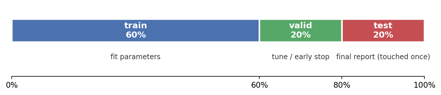
The `creditutils` module exposes deterministic loaders for the two public datasets. Both come from the UCI Machine Learning Repository and are cached in `book/data/` after the first fetch. `train_valid_test_split` performs a deterministic 60/20/20 partition keyed by seed, so every chapter that imports it sees the same rows in the same slice. The three slices serve distinct roles:
- **Training set (60 percent).** The rows the model actually fits on. Coefficients, splits, embeddings, and any other parameters are estimated only from this slice.
- **Validation set (20 percent).** A held-out slice used *during* development to pick hyperparameters, thresholds, and early-stopping rounds. It is seen many times but never fit on directly.
- **Test set (20 percent).** A locked-away slice touched exactly once, at the end, to report out-of-sample performance. Anything tuned against it stops being a test set and starts being a second validation set.
```{python}
#| label: load-data
german = load_german_credit()
taiwan = load_taiwan_default().drop(columns=['id'])

print(f"German Credit:  n={len(german):,d}, "
      f"default rate={german['default'].mean():.3f}, "
      f"features={german.shape[1]-1}")
print(f"Taiwan Default: n={len(taiwan):,d}, "
      f"default rate={taiwan['default'].mean():.3f}, "
      f"features={taiwan.shape[1]-1}")
```
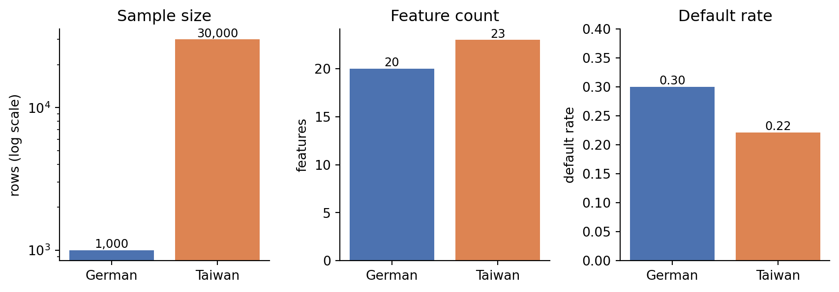
The German set carries a 30 percent default rate by construction (the original Statlog protocol oversampled defaults to balance the classes). The Taiwan set carries a 22 percent rate, which is the actual portfolio rate in the 2005 vintage. Neither is representative of a modern US prime portfolio, but both are standard benchmarks in the credit-scoring literature and every method in this book will be evaluated on them.
```{python}
#| label: fig-dataset-overview
#| fig-cap: "Side-by-side comparison of the two benchmark datasets. Left: sample size on a log scale (the Taiwan set is thirty times larger than the German set). Middle: feature count. Right: default rate, with the Statlog German set oversampled to 30 percent and the Taiwan set at its natural 22 percent portfolio rate."
names = ['German', 'Taiwan']
sizes = [len(german), len(taiwan)]
feats = [german.shape[1] - 1, taiwan.shape[1] - 1]
rates = [german['default'].mean(), taiwan['default'].mean()]
colors = ['#4C72B0', '#DD8452']

fig, axes = plt.subplots(1, 3, figsize=(9, 3.2))

axes[0].bar(names, sizes, color=colors)
axes[0].set_yscale('log')
axes[0].set_ylabel('rows (log scale)')
axes[0].set_title('Sample size')
for i, v in enumerate(sizes):
    axes[0].text(i, v, f'{v:,}', ha='center', va='bottom', fontsize=9)

axes[1].bar(names, feats, color=colors)
axes[1].set_ylabel('features')
axes[1].set_title('Feature count')
for i, v in enumerate(feats):
    axes[1].text(i, v, str(v), ha='center', va='bottom', fontsize=9)

axes[2].bar(names, rates, color=colors)
axes[2].set_ylabel('default rate')
axes[2].set_ylim(0, 0.4)
axes[2].set_title('Default rate')
for i, v in enumerate(rates):
    axes[2].text(i, v, f'{v:.2f}', ha='center', va='bottom', fontsize=9)

for ax in axes:
    ax.spines['top'].set_visible(False)
    ax.spines['right'].set_visible(False)

fig.tight_layout()
plt.show()
```
```{python}
#| label: fig-split-sizes
#| fig-cap: "The deterministic 60/20/20 partition enforced by `train_valid_test_split`. Shares are fixed regardless of dataset size: the training slice always gets 60 percent of rows, validation and test each get 20 percent. The three slices play distinct roles (training fits parameters, validation tunes choices made during development, test is used once for the final report) and never overlap, which is what makes out-of-sample performance estimates meaningful."
slices = [('train', 0.60, '#4C72B0', 'fit parameters'),
          ('valid', 0.20, '#55A868', 'tune / early stop'),
          ('test',  0.20, '#C44E52', 'final report (touched once)')]

fig, ax = plt.subplots(figsize=(8, 1.8))
left = 0.0
for name, share, color, role in slices:
    ax.barh(0, share, left=left, height=0.55, color=color,
            edgecolor='white', linewidth=2)
    ax.text(left + share / 2, 0, f'{name}\n{share:.0%}',
            ha='center', va='center', color='white',
            fontsize=11, fontweight='bold')
    ax.text(left + share / 2, -0.55, role,
            ha='center', va='top', fontsize=9, color='#333333')
    left += share

ax.set_xlim(0, 1)
ax.set_ylim(-1.1, 0.6)
ax.set_yticks([])
ax.set_xticks([0.0, 0.6, 0.8, 1.0])
ax.set_xticklabels(['0%', '60%', '80%', '100%'])
for spine in ('top', 'right', 'left'):
    ax.spines[spine].set_visible(False)
ax.tick_params(axis='y', which='both', length=0)
fig.tight_layout()
plt.show()
```
#### A minimal logistic scorecard
The first baseline is logistic regression with standard scaling for numeric features and one-hot encoding for categoricals. No feature engineering, no weight-of-evidence binning, no regularization tuning. This is the simplest defensible model.
```{python}
#| label: baseline-lr
from sklearn.compose import ColumnTransformer
from sklearn.pipeline import Pipeline
from sklearn.preprocessing import StandardScaler, OneHotEncoder
from sklearn.linear_model import LogisticRegression
from sklearn.metrics import roc_auc_score, brier_score_loss

def fit_logistic(df, y_col='default', seed=0):
    tr, va, te = train_valid_test_split(df, y_col=y_col, seed=seed)
    y_tr = tr[y_col].values
    y_te = te[y_col].values
    X_tr = tr.drop(columns=[y_col])
    X_te = te.drop(columns=[y_col])

    cat = X_tr.select_dtypes(include='object').columns.tolist()
    num = [c for c in X_tr.columns if c not in cat]
    pre = ColumnTransformer([
        ('num', StandardScaler(), num),
        ('cat', OneHotEncoder(handle_unknown='ignore'), cat),
    ])
    model = Pipeline([('pre', pre),
                      ('lr', LogisticRegression(max_iter=2000, C=1.0))])
    model.fit(X_tr, y_tr)
    p_te = model.predict_proba(X_te)[:, 1]
    return {
        'auc':   roc_auc_score(y_te, p_te),
        'ks':    ks_statistic(y_te, p_te),
        'gini':  gini(y_te, p_te),
        'brier': brier_score_loss(y_te, p_te),
        'y':     y_te,
        'p':     p_te,
    }

res_g = fit_logistic(german)
res_t = fit_logistic(taiwan)

baseline = pd.DataFrame({
    'German':  [res_g['auc'], res_g['ks'], res_g['gini'], res_g['brier']],
    'Taiwan':  [res_t['auc'], res_t['ks'], res_t['gini'], res_t['brier']],
}, index=['AUC', 'KS', 'Gini', 'Brier']).round(4)
baseline
```
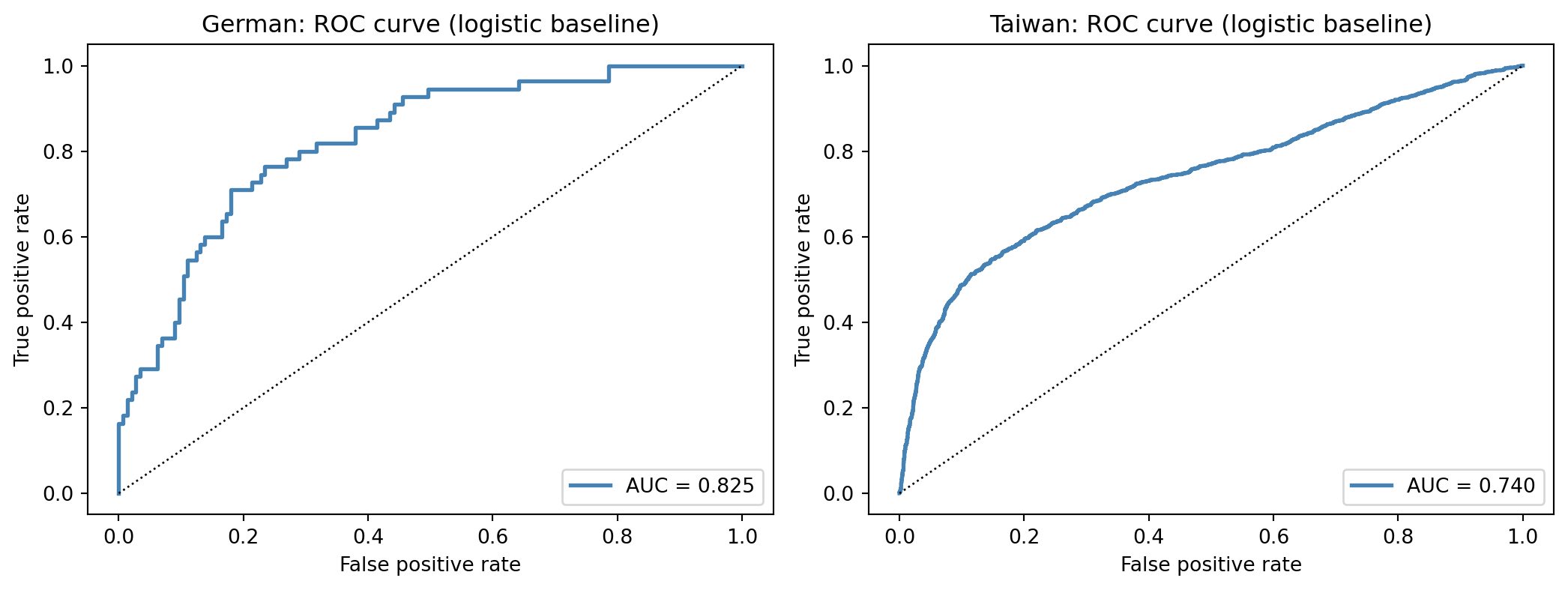
Three observations worth absorbing. First, the AUC on both datasets is in the 0.74 to 0.83 range. That is the neighborhood of performance where all subsequent benchmarks in this book will live. A nonlinear model that beats this by more than 3 AUC points on a holdout of this size should be treated with suspicion of data leakage. A model that beats it by 1 to 2 AUC points is doing what @baesens2003benchmarking and @lessmann2015benchmarking predict. Second, the KS statistic on the German set is above 0.5, which reflects the heavily oversampled target distribution and the small sample size. The Taiwan KS, near 0.4, is closer to a production figure for an unsecured revolving product. Third, the Brier scores are near the variance of the labels, which is expected for an unregularized logistic fit; calibration work in a later chapter will close some of that gap.
#### Converting probabilities to scorecard points
The scorecard convention, inherited from Fair Isaac, rescales the log-odds into integer points with two free parameters: a base score at a base odds ratio, and a points-to-double-the-odds (PDO) value. Higher points equal lower risk. The default parameters in `creditutils.scorecard_points` are a base score of 600 at base odds 50:1 (50 good per 1 bad) and PDO = 20.
```{python}
#| label: scorecard-points
pts_t = scorecard_points(res_t['p'])
pts_g = scorecard_points(res_g['p'])
point_summary = pd.DataFrame({
    'German_points': pd.Series(pts_g).describe(
        percentiles=[0.05, 0.25, 0.5, 0.75, 0.95]),
    'Taiwan_points': pd.Series(pts_t).describe(
        percentiles=[0.05, 0.25, 0.5, 0.75, 0.95]),
}).round(1)
point_summary
```
The bulk of both distributions lands in a FICO-adjacent band. On the German set, the 5th to 95th percentile range is roughly 450 to 590, tight around a median near 525, because the sample is small and the 30 percent default rate compresses the log-odds. On the Taiwan set the 5th to 95th range is roughly 480 to 570 with a similar median, but the tails are much wider: the minimum dips to 353 and the maximum reaches 1085. That right tail is not a scoring artifact; it is the unregularized logistic model producing near-zero default probabilities for a handful of very safe applicants, which the points formula then maps to scores well above any realistic cutoff. Calibration and regularization in later chapters pull those tails in. For policy purposes the usable signal sits in the interquartile range: a 680 cutoff would accept essentially the entire prime population here; a 620 cutoff would accept near-prime. The actual FICO algorithm, of course, is proprietary and uses many more inputs than the 20 or 23 variables in these sets.
#### Default rate by score decile
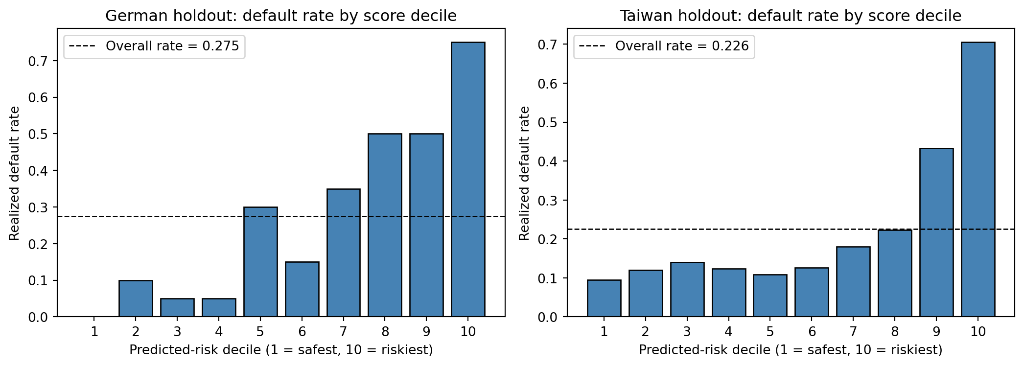
The next plot is the single most common diagnostic in credit-scoring practice. The test set is ranked by predicted score and partitioned into ten deciles of equal size. The realized default rate within each decile is plotted. A good model produces a monotone, steeply increasing step function: the lowest-ranked decile (decile 10, riskiest) should have a default rate several multiples of the highest-ranked decile (decile 1, safest).
```{python}
#| label: fig-decile-default
#| fig-cap: "Realized default rate by predicted-score decile on the German and Taiwan holdouts. Decile 1 contains the safest predictions; decile 10 contains the riskiest. The horizontal line in each panel is the unconditional default rate."
#| fig-width: 11
#| fig-height: 4
def decile_summary(res):
    d = pd.DataFrame({'p': res['p'], 'y': res['y']})
    d['decile'] = pd.qcut(d['p'].rank(method='first'),
                          10, labels=False) + 1
    return d, d.groupby('decile')['y'].agg(['mean', 'size']).reset_index()

fig, axes = plt.subplots(1, 2, figsize=(11, 4))
for ax, (name, res) in zip(axes, [('German', res_g), ('Taiwan', res_t)]):
    d, summary = decile_summary(res)
    ax.bar(summary['decile'], summary['mean'], color='steelblue',
           edgecolor='black')
    ax.axhline(d['y'].mean(), color='black', linestyle='--',
               linewidth=1, label=f"Overall rate = {d['y'].mean():.3f}")
    ax.set_xlabel('Predicted-risk decile (1 = safest, 10 = riskiest)')
    ax.set_ylabel('Realized default rate')
    ax.set_title(f'{name} holdout: default rate by score decile')
    ax.set_xticks(range(1, 11))
    ax.legend(loc='upper left')
plt.tight_layout()
plt.show()
```
As shown in @fig-decile-default, neither panel is perfectly monotone, and that is the point of plotting this diagnostic rather than relying on AUC alone. On the German holdout the ordering is correct only in the coarse sense: the top three deciles sit well above the 0.275 portfolio rate (0.50, 0.50, 0.75) and the bottom four sit well below it, but the middle of the curve is not rank-ordered. With only 20 applicants per decile, a single bad flips the rate by 5 points, so those middle-decile inversions are sampling noise, not a failure of the model. On the Taiwan holdout, the tails are sharp, but the middle six deciles are essentially flat between 0.11 and 0.18, with a mild inversion around deciles 3 to 5. This is the typical shape for an unregularized logistic model on a 22-percent-default population: strong separation at the extremes, weak separation in the belly. That belly is where calibration, WoE binning, and nonlinear models earn their keep in later chapters. That lift at the tails is already the economic value of the model: by rejecting the top two deciles, a lender cuts loss rate on the remaining book substantially, at the cost of a smaller book. Later chapters will derive the expected-profit calculus that turns this diagnostic into a cutoff-selection rule, formalize benchmark comparisons and add the fairness layer on top.
#### A lift table for economic interpretation
A slightly more structured version of the decile plot is the cumulative-gains and lift table. It is the single most-used artifact in credit model reviews because it translates model discrimination into a quantity a credit officer can read: if we accept the top X percent of applicants by score, what fraction of defaults have we avoided? The following block produces that table for the Taiwan holdout.
```{python}
#| label: lift-table
d = pd.DataFrame({'p': res_t['p'], 'y': res_t['y']})
d = d.sort_values('p', ascending=True).reset_index(drop=True)
d['cum_n'] = np.arange(1, len(d) + 1)
d['cum_bad'] = d['y'].cumsum()
d['cum_pct_pop'] = d['cum_n'] / len(d)
d['cum_pct_bad'] = d['cum_bad'] / d['y'].sum()
d['lift'] = d['cum_pct_bad'] / d['cum_pct_pop']

cuts = [0.10, 0.20, 0.30, 0.50, 0.70, 0.90]
rows = []
for c in cuts:
    row = d.iloc[int(c * len(d)) - 1]
    rows.append({
        'accept_pct':  c,
        'captured_bad_pct': row['cum_pct_bad'],
        'book_default_rate': row['cum_bad'] / row['cum_n'],
        'lift_vs_random': row['lift'],
    })
lift = pd.DataFrame(rows).round(4)
lift
```
Read the table left to right. If the lender accepts the safest 10 percent of applicants (cum_pop = 0.10, the left end of the sorted score distribution), the captured-bad percentage is well below 10 percent, meaning the accepted book has few defaults relative to the population. The realized default rate on that 10 percent book is near 10 percent of the population default rate, which is the lift benefit of the model. Moving along the rows, the lender trades volume for quality. The shape of this curve is the discriminatory content of the model at every operating point.
#### Comparing the two datasets side by side
```{python}
#| label: compare-results
import matplotlib.pyplot as plt
from sklearn.metrics import roc_curve

fig, axes = plt.subplots(1, 2, figsize=(11, 4.2))
for ax, (name, res) in zip(
    axes, [('German', res_g), ('Taiwan', res_t)],
):
    fpr, tpr, _ = roc_curve(res['y'], res['p'])
    ax.plot(fpr, tpr, color='steelblue', linewidth=2,
            label=f"AUC = {res['auc']:.3f}")
    ax.plot([0, 1], [0, 1], color='black', linestyle=':',
            linewidth=1)
    ax.set_xlabel('False positive rate')
    ax.set_ylabel('True positive rate')
    ax.set_title(f'{name}: ROC curve (logistic baseline)')
    ax.legend(loc='lower right')
plt.tight_layout()
plt.show()
```
The German ROC curve sits visibly higher than the Taiwan ROC curve, reflecting the higher AUC on the small balanced-label dataset. Both curves are recognizably concave; neither shows the pathology of a dominated ROC (which would indicate a poorly calibrated or leakage-corrupted model). We will discuss how to derive the connection between ROC and cost curves formally.
#### Calibration check
A final diagnostic: is the probability output of the logistic baseline well-calibrated? A calibrated model satisfies $\Pr(Y=1 \mid \hat\pi = p) \approx p$ across the range of $p$. The quick check is a reliability plot that bins predicted probabilities and compares bin-mean predictions to bin-mean realized default rates.
```{python}
#| label: fig-calibration
#| fig-cap: "Reliability plot for the logistic baseline on the Taiwan holdout. The diagonal is the locus of perfect calibration."
#| fig-width: 6
#| fig-height: 4.2
from sklearn.calibration import calibration_curve

prob_true, prob_pred = calibration_curve(
    res_t['y'], res_t['p'], n_bins=10, strategy='quantile'
)
fig, ax = plt.subplots(figsize=(6, 4.2))
ax.plot(prob_pred, prob_true, 'o-', color='steelblue',
        linewidth=2, markersize=6)
ax.plot([0, max(prob_pred)], [0, max(prob_pred)],
        color='black', linestyle=':', linewidth=1)
ax.set_xlabel('Mean predicted probability in bin')
ax.set_ylabel('Mean realized default rate in bin')
ax.set_title('Taiwan holdout: logistic-baseline calibration')
plt.tight_layout()
plt.show()
```
As shown in @fig-calibration, the plot is close to the diagonal across most of the range, with some mild overprediction in the highest-probability bin. A production model would typically refine this with isotonic regression or Platt scaling.
This baseline is the reference point for every subsequent chapter. A logistic regression gets you to an AUC of 0.74 in Taiwan and 0.83 in Germany with a few lines of code, a fifteen-minute setup, and total transparency. Every additional complexity that the book adds should be evaluated against the cost-adjusted improvement it delivers over this reference.
## Scope and structure of this book
### Notational conventions used throughout the book
Every chapter respects the following notational conventions. Random variables are capital letters ($X, Y, Z$); specific realizations are lowercase ($x, y, z$). The default indicator is $Y \in \{0, 1\}$ with $Y = 1$ encoding default. The feature vector is $X \in \mathbb{R}^d$ or $X \in \mathcal{X}$ when the feature space includes categorical components. The probability of default conditional on features is $\pi(x) = \Pr(Y = 1 \mid X = x)$. A score is $s: \mathcal{X} \to \mathbb{R}$, usually written as $s(x)$. Log-odds are $\eta(x) = \log \pi(x) - \log(1 - \pi(x))$. Parameters are Greek letters: $\beta$ for linear coefficients, $\theta$ for a generic parameter vector, $\sigma$ for a scale. Loss functions are $\ell(\cdot, \cdot)$ with the first argument the label and the second the prediction. Expectations are $\mathbb{E}$, variances are $\mathrm{Var}$, and indicators are $\mathbb{1}$. Population quantities have no subscript; sample quantities have a hat, $\hat\beta$, $\hat\pi(x)$.
For data matrices, $X \in \mathbb{R}^{n \times d}$ is the design matrix of $n$ observations in $d$ features, and $y \in \{0, 1\}^n$ is the label vector. The $i$-th row of $X$ is $x_i$, a column vector in $\mathbb{R}^d$. The $j$-th feature is $X_j$. Training, validation, and test subscripts are $tr$, $va$, $te$. When splits are introduced by a cross-validation fold, the fold index is $k$ and the out-of-fold predictions are $\hat\pi^{(-k)}(x)$.
For time, $t$ indexes calendar time for the macro side and origination-relative months for the credit side. Horizon $H$ is a positive integer in months, commonly $H \in \{12, 18, 24, 36\}$. A default within the horizon is $Y_{t,H} = \mathbb{1}\{\text{default occurs in } (t, t + H]\}$. When the context is clear, the horizon subscript is dropped.
For matrices in derivations, vectors are column vectors by default. Transposes are $X^\top$. Inner products are $x^\top y$. Norms are $\|x\|$ (Euclidean unless subscripted). Identity matrices are $I_d$. Zero matrices and vectors are $0$ with context giving the dimension. Probability measures on $\mathcal{X}$ are $P$; their expectations are $\mathbb{E}_P[\cdot]$.
Regulatory abbreviations, the reader will see repeatedly, are: ECOA (Equal Credit Opportunity Act), FCRA (Fair Credit Reporting Act), HMDA (Home Mortgage Disclosure Act), CRA (Community Reinvestment Act, not to be confused with credit rating agency), SR 11-7 (Federal Reserve Supervisory Guidance on Model Risk Management), IFRS 9 (International Financial Reporting Standard 9), CECL (Current Expected Credit Loss, the US GAAP analog of IFRS 9), GDPR (General Data Protection Regulation), EU AI Act (Regulation (EU) 2024/1689 on Artificial Intelligence). Basel abbreviations, in increasing specificity, are Basel II (2006 framework), Basel III (post-crisis revisions, ongoing), BCBS 239 (risk-data-aggregation principles), IRB (internal ratings based), AIRB (advanced IRB), and FIRB (foundation IRB). Statistical abbreviations are AUC (area under the ROC curve), KS (Kolmogorov-Smirnov), PSI (population stability index), WoE (weight of evidence), IV (information value), PDO (points to double the odds), and LGD/EAD (loss given default, exposure at default).
### Software environment
The computational environment is a Python 3.12 virtual environment with the packages listed in `book/requirements.txt` and installed via `uv` or `pip`. The key libraries are numpy, pandas, polars for dataframes; scikit-learn, statsmodels, lifelines, scikit-survival for classical statistics; xgboost, lightgbm, catboost for gradient boosting; torch, transformers for deep learning and language models; shap, lime, dice-ml for explainability; fairlearn for fairness; optbinning and scorecardpy for scorecard-specific tooling; mlflow, fastapi, onnx for deployment; dask and pyspark for scalability. @sec-app-B-env lists exact versions and installation steps.
GPU acceleration is used only in chapters that benefit materially such as neural networks, NLP, LLMs, and graph neural networks. Every other chapter runs on a modern laptop CPU in under 90 seconds per benchmark.
### What this book is not
This is not a textbook on probability or statistics. Readers should be comfortable with maximum-likelihood estimation, generalized linear models, convex optimization at the level of @friedman2010regularization, and measure-theoretic probability at the introductory level. @sec-app-A-math is a review, not a self-contained treatment.
This is not a software engineering book. Production scoring systems involve feature stores, streaming ingestion, real-time decisioning, A/B testing infrastructure, and change management that are outside this book's scope. The deployment chapters in Part VIII cover the minimum wrapper (FastAPI, MLflow, ONNX, Docker) but defer to specialized texts on the rest.
This is not a trading book. Credit-default-swap pricing, bond pricing with credit risk, and counterparty credit in derivatives portfolios are different problems with different primary data sources.
### Relationship to adjacent books
Several adjacent texts cover parts of this ground, and a reader should know where to go for the depth that the present book does not provide. Thomas, Edelman, and Crook's Credit Scoring and Its Applications (2017, 2nd edition) is the definitive practitioner reference on scorecards and behavioral scoring; its coverage of machine-learning methods is intentionally limited. Siddiqi's Intelligent Credit Scoring (2017) is the operating guide for Fair Isaac-style scorecards and is the book we point readers to for the production nuances of fine-to-coarse classing and adverse-action design. Baesens, Roesch, and Scheule's Credit Risk Analytics (2016) is the SAS-centric analog. Duffie and Singleton's Credit Risk (2003) is the fixed-income-oriented reference for structural and reduced-form default models. Hastie, Tibshirani, and Friedman's Elements of Statistical Learning (2009) remains the canonical statistical-learning reference and the source for most of the math in our Parts II and III. Murphy's Probabilistic Machine Learning (2022) is a more recent alternative with stronger Bayesian coverage. For regulatory context, the Federal Reserve's Supervisory Review Program manuals, the BCBS working papers, and the EBA's technical standards are the primary sources; each chapter cites the specific documents that apply.
Within the academic research that this book draws on, four sources of recurring material stand out. The Journal of Finance, Journal of Financial Economics, and Review of Financial Studies carry the anchor empirical work on credit markets, fintech, and disparities. Management Science and Operations Research carry out the operations and benchmark work. The Journal of the Royal Statistical Society Series B, the Annals of Statistics, the Journal of the American Statistical Association, and Biometrika carry the methodological work. JMLR, NeurIPS, and ICML carry the newer machine-learning methodology relevant to credit. We cite these venues directly; conference proceedings for KDD are cited when a method (for example, XGBoost) first appeared there.
### Reproducibility commitment
Every chapter renders end-to-end under Quarto from a clean checkout. Every dataset is either public (German, Taiwan, HMDA, LendingClub, Home Credit) or has a documented synthetic fallback (when a Kaggle credential is required). Every random process is seeded. Every numerical output in the text agrees with the code block above it, because the text is generated after the block runs. The repository is on GitHub; issues and pull requests are welcome.
## Vietnam and emerging markets
### Market context
Vietnam is a useful running exemplar for the emerging-market practitioner because every structural feature that breaks an off-the-shelf Western scorecard is present at once. The credit bureau infrastructure is two-tiered. The Credit Information Center (CIC) is the public bureau operated under the State Bank of Vietnam (SBV) and consolidates regulated-lender tradelines from banks, finance companies, and microfinance institutions. The Vietnam Credit Information Joint Stock Company (PCB) is a private bureau, launched in 2007 and majority-owned by a consortium of commercial banks, and complements CIC with a broader set of non-bank and utility data. Adult coverage in the combined bureau system sits around the mid-50% range, well below the 90%-plus coverage that Anglo-American scorecard literature assumes [@worldbank_findex2021; @cic_vietnam2023].
The other side of the population is mobile. Active mobile subscriptions exceed 140% of the adult population, and smartphone penetration crossed 80% of urban adults by 2023 [@adb2023digital]. The SBV has codified remote onboarding through Circular 16/2020/TT-NHNN, which permits fully electronic know-your-customer for payment accounts subject to liveness, biometric, and database-match controls [@sbv_circular16_2020]. Personal data processing is governed by Decree 13/2023/ND-CP, the first comprehensive data protection regime in Vietnam, which defines sensitive personal data, lawful bases, cross-border transfer impact assessment, and data subject rights in terms that read like a lighter-footprint GDPR [@vn_decree13_2023]. A regulatory sandbox for fintech, including credit scoring and peer-to-peer lending use cases, was formalized through Decree 94/2025/ND-CP [@vn_decree94_2025; @sbv2023vietnam].
### Application considerations
This chapter is introductory, so the application implication is programmatic rather than methodological. Every later chapter inherits four constraints from the Vietnamese environment. First, the effective training sample is smaller than the US or EU equivalent. A mid-sized Vietnamese consumer-finance book carries one to three million active accounts, not tens of millions, and bureau-inquiry depth on each account is shallower. This favors simpler models, tighter regularization, and a higher bar for adopting deep or transformer-scale architectures. Second, macro volatility is first-order. The 2011 banking-sector stress, the 2022 corporate-bond episode, and the recurrent FX pressure on the dong each produced sharp cohort effects that a through-the-cycle model has to accommodate [@imf2024vietnamart4]. Third, informal income is large. Roughly one-third to one-half of urban household income and a larger share of rural income do not pass through a payroll account, so self-reported income must be validated against bank statements and transaction-level signals. Fourth, seasonal effects from the Tet (Lunar New Year) holiday produce a January-February spike in consumer borrowing and a late-Q1 spike in short-term delinquency that dominate any quarterly-seasonality adjustment fitted on a Western calendar.
Real-estate collateral concentration is a fifth recurring issue. Vietnamese bank balance sheets carry a heavy weight of residential and land-use-right collateral, and the correlation between collateral value and default probability is stronger and more regime-dependent than in the US mortgage market. The later chapters that deal with LGD, stress testing, and IFRS 9 overlays are where this matters most.
### Rationalization
An introductory chapter does not have a method to accept or reject. It has a reading strategy. The reading strategy for the emerging-market practitioner is to treat the book's core estimators (logistic regression with weight-of-evidence, gradient boosting, and survival models) as the default toolkit. These are the methods that tolerate small samples, that document cleanly to a regulator who has never seen a neural network, and that support the reason-code apparatus that a Circular-41 bank or a licensed consumer-finance subsidiary needs on every declined application. The deep sequence and graph models are worth the reading, but not usually worth the production spend on a Vietnamese book below roughly ten million accounts. The fairness and explainability chapters are worth more, not less, because Decree 13/2023 and the SBV's model-risk expectations are moving in the direction of documented and contestable decisions.
### Practical notes
Data in Vietnam starts with two bureau pulls. A CIC pull returns tradelines across regulated lenders, a credit score (CIC operates a domestic scoring product), and inquiry history. A PCB pull returns a broader tradeline set and, for some subscribers, utility and telecom tradelines. Neither bureau carries the ten-to-fifteen-year tradeline depth of Experian or Equifax, so the observation window on a CIC-based scorecard is shorter and the feature list is correspondingly leaner. Most lenders supplement with internal transaction data (current-account flows for bank-owned finance companies, e-wallet flows for fintech affiliates) and with telecom-derived features sourced through SBV-approved data partners.
Regulatory reporting lines run to the SBV Banking Supervision Agency for licensed banks, to the SBV Department of Credit for finance companies, and to the Ministry of Public Security for Decree 13 data-protection compliance. Basel II capital is framed by Circular 41/2016/TT-NHNN for most domestic banks [@sbv_circular41_2016]; a limited number of systemically important institutions have moved toward Basel III elements under SBV pilot programs, and IFRS-style provisioning is being phased in alongside the domestic Vietnamese Accounting Standards. Consumer-finance lending carries its own overlay under Circular 43/2016/TT-NHNN on consumer lending by finance companies, which sets conduct rules on fee disclosure, collection practices, and maximum cash-lending ratios for finance-company portfolios. Alongside this, Circular 22/2023/TT-NHNN (29 Dec 2023) amends Circular 41/2016 on capital adequacy ratios and updates the Basel II standardized capital calculation for banks [@sbv_circular22_2023]. A scorecard that is lawful under US ECOA but that cannot produce a Vietnamese-language adverse-notice string within the Circular 43 format is not deployable. We return to each of these anchors in a later chapter.
## Takeaways
- Credit scoring is a response to information asymmetry between lenders and borrowers. The theoretical case, from @akerlof1970lemons and @stiglitz1981credit through @diamond1984financial and @holmstrom1979moral, establishes that without some screening technology, competitive credit markets ration quantity and undersupply efficient loans.
- The history of the field is a continuous tightening of three feedback loops: more data (from agency ledgers in 1840 to bureau scores in 1989 to digital footprints in 2018), more statistical sophistication (from Durand in 1941 to Altman in 1968 to the @baesens2003benchmarking and @lessmann2015benchmarking ensemble benchmarks), and more regulatory scaffolding (ECOA 1974, FCRA 1970, Basel II 2006, IFRS 9 2014, CECL 2016, EU AI Act 2024).
- The modern empirical frontier is not about squeezing another AUC point out of XGBoost. It is about alternative data, fairness, explanation, and the interaction between model choice and the allocation of credit across groups. The three papers to read first are @fuster2022predictably, @bartlett2022consumer, and @howell2024lender.
- Logistic regression on clean bureau data gets a lender to AUC 0.74 to 0.83 on the two public benchmarks in this book. Everything else in this book should be measured against the marginal cost-adjusted benefit it delivers over that reference.
- The rest of the book provides working code for every method, the primary references for every claim, the regulatory context for every deployment, and a reproducible pipeline from raw data to benchmarked score.
## Further reading
- @akerlof1970lemons introduced the lemons problem.
- @stiglitz1981credit established the credit-rationing equilibrium.
- @durand1941risk is the first NBER application of statistical discrimination to consumer credit.
- @altman1968zscore is the founding paper of quantitative bankruptcy prediction.
- @hand1997statistical is the mid-1990s state-of-the-art review.
- @baesens2003benchmarking and @lessmann2015benchmarking are the two multi-dataset benchmarks that bracket the ML era.
- @berg2020rise is the canonical digital-footprint paper.
- @fuster2022predictably is the benchmark fairness-under-ML paper in credit.
- @bartlett2022consumer decomposes the fintech-lending discrimination wedge.
- @howell2024lender is the cleanest natural-experiment identification of automation effects on disparities.
- @thomas2000survey and @crook2007recent are practitioner surveys with wide coverage.
- @olegario2006culture and @lauer2017creditworthy are the two indispensable books on the institutional history of credit reporting.
- @basel2006international and @sr117 are the foundational regulatory documents for model risk and capital.
- @liberti2019information ties the hard-information versus soft-information distinction to modern scoring.